Cosmology with Gamma Ray Bursts

Abstract

Apparently, Gamma–Ray Bursts (GRBs) are all but standard candles. Their emission is collimated into a cone and the received flux depends on the cone aperture angle. Fortunately we can derive the aperture angle through an achromatic steepening of the lightcurve of the afterglow, and thus we can measure the “true” energetics of the prompt emission. Ghirlanda et al. (2004) found that this collimation–corrected energy correlates tightly with the frequency at which most of the radiation of the prompt is emitted. Through this correlation we can infer the burst energy accurately enough for a cosmological use. Using the best known 15 GRBs we find very encouraging results that emphasize the cosmological GRB role. Probing the universe with high accuracy up to high redshifts, GRBs establish a new insight on the cosmic expanding acceleration history and accomplish the role of “missing link” between the Cosmic Microwave Background and type Ia supernovae, motivating the most optimistic hopes for what can be obtained from the bursts detected by SWIFT.

1 Introduction

The huge emitted power of Gamma Ray Bursts (GRBs) makes them detectable at any redshift $z<20$. It is therefore natural to use them as probes of the far universe, to explore the epoch of reionization (see e.g. [2], [11]) and to study the properties of the material between them and us, through the study of absorption lines in the spectra of their prompt emission and afterglow. Furthermore, as it seems very likely, GRBs are intimately connected with the formation of massive stars, and through GRBs we hope to shed light on the star formation history at unprecedented redshifts, without the limitation of extinction which may plague samples of distant galaxy resulting from deep surveys ([6], see also Firmani et al. in these proceedings). However, until now, the hopes to use them as standard candles to measure the geometry and kinematics of our universe have been frustrated by the large dispersion of their energetics, even when corrected for collimation ([5]; [3]). This changed with the findings by Ghirlanda et al. (2004a, hereafter GGL, see also Ghirlanda et al. in these proceedings) that the spectral properties of GRBs are related with the energy radiated within their collimation cones. This correlation is tight enough to allow the most optimistic hopes for the cosmological use of GRBs in the SWIFT era. This “Ghirlanda” correlation links the energy $E_{\rm peak}$ where most of the prompt radiation is emitted with the total energy $E_{\gamma}$ radiated during the prompt phase of a GRB. Since the emission is collimated into a cone, $E_{\gamma}$ is not simply measured by the received fluence. To find it, one needs to measure the semi–aperture cone angle, through the achromatic break in the lightcurve of the afterglow. The Ghirlanda correlation is very similar to the “stretching” relation of SN Ia ([13]): more powerful SN Ia have lightcurves that decay more slowly. The Ghirlanda relation is then a sort of Cepheid–like relation: even if the collimation–corrected energetics of GRBs are not all equal (i.e. they are not standard candles in the strict sense), we have a tool to know each of them (GRBs become “known candles”).

2 The Hubble diagram

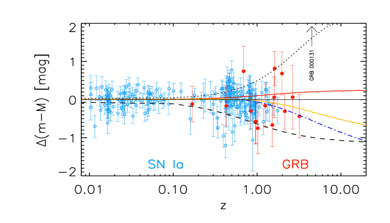
Figure 1: Residuals of the distance moduli of SNe Ia and of the 15 GRBs with known redshift and collimation angle with respect to the case $\Omega_{\rm M}$=0.27, $\Omega_{\Lambda}$=0.73. Also shown are the differences of various other cosmological models with respect to the $\Omega_{\rm M}$=0.27, $\Omega_{\Lambda}$=0.73  case: red solid line: $\Omega_{\rm M}$=0.2, $\Omega_{\Lambda}$=0.8; orange solid line: $\Omega_{\rm M}$=0.37, $\Omega_{\Lambda}$=0.85; blue dot–dashed line: $\Omega_{\rm M}$=0.45, $\Omega_{\Lambda}$=0.95; black dashed line: $\Omega_{\rm M}$=1, $\Omega_{\Lambda}$=0; black dotted line: $\Omega_{\rm M}$=0.01, $\Omega_{\Lambda}$=0.99. The arrow marks the redshift of GRB 000131 ($z$=4.5) which is the most distant GRB of known $z$. From [7].

Fig. 1 shows the Hubble diagram in the form of residuals with respect to the specific choice of $\Omega_{\rm M}$=0.27  and $\Omega_{\Lambda}$=0.73, for SNe Ia and GRBs, together with different lines corresponding to different $\Omega_{\rm M}$, $\Omega_{\Lambda}$ pairs. Since it is likely that GRBs follow the star formation history, it is also very likely that they exist up to $z\sim$10–20. Even at these redshifts, GRBs are easily detectable. Note that the error bars of GRBs are slightly larger than the error bars of SN Ia, but note also that the maximum redshifts already measured of GRBs is $z=4.5$, while SN Ia extends up to a maximum redshift of 1.7. This is also the maximum foreseen value of the future SNAP satellite, designed to accurately find and observe distant supernovae to accurately constrain cosmological parameters and models. Needless to say, it is highly desirable to have more than one class of standard (or known) candles, to cancel possible evolutionary effects (which are likely different for different classes of objects) and to cure possible extinction effects (for GRBs, the hard X–rays of their prompt emission are virtually unaffected by absorption).

The crucial issue about the use of the Ghirlanda relation for cosmology is what can be called the “circularity problem”: to find slope and normalization of the correlation, we are obliged to choose a particular cosmology (i.e. a particular pair of $\Omega_{\rm M}$, $\Omega_{\Lambda}$ values). The correlation has not (yet) been calibrated with low–redshifts GRBs, unaffected by the choise of $\Omega_{\rm M}$ and $\Omega_{\Lambda}$, simply because low redshift GBRs are very few, and we may wait for years (even with SWIFT) before building a sample numerous enough of low–$z$ GRBs. In the meantime, we have to deal with the circularity problem, and in the next section we will describe the 4 existing methods already suggested.

3 How to cure the circularity problem

The Ghirlanda relation has already been used to find constraints on the cosmological parameters. We briefly describe here the four methods that have been proposed and used. In principle, the cosmological parameters to find are not only $\Omega_{\rm M}$ and $\Omega_{\Lambda}$, but also the parameter $w$ entering in the equation of state of the dark energy $P=w\rho c^{2}$ where $P$ and $\rho$ are the pressure and energy density of the dark energy. Note that $w$ can be assumed constant or be a function of redshift. One possible parametrization is $w=w_{0}+w^{\prime}z$. The cosmological $\Lambda$ term corresponds to $w_{0}=-1$ and $w^{\prime}=0$. Consider for simplicity this latter case. To the aim to put constraints on $\Omega_{\rm M}$ and $\Omega_{\Lambda}$, the basic ideas of the four methods are the following:

1. Dai et al. (2004) assumed that the $E_{\rm peak}$–$E_{\gamma}$ correlation found using a given pair of ($\Omega_{\rm M}$, $\Omega_{\Lambda}$) values was cosmology independent. In other words, Dai et al. (2004) assumed that the slope of the correlation is fixed (they used $E_{\gamma}\propto E_{\rm peak}^{3/2}$). Instead, this slope corresponds to a specific choice of $\Omega_{\rm M}$, $\Omega_{\Lambda}$. This method could be applied if there is a robust theoretical interpretation of the Ghirlanda relation, putting an heavy weight to a given slope and normalization of the correlation.

2. Ghirlanda et al. (2004b, GGLF hereafter), pointing out the circularity problem of the Dai et al. approach, proposed instead to use the scatter around the fitting line of the $E_{\rm peak}$–$E_{\gamma}$ correlation as an indication of the best cosmology. In other words, they find a given Ghirlanda correlation using a pair of $\Omega_{\rm M}$, $\Omega_{\Lambda}$, and measure the scatter of the points around this correlation through a $\chi^{2}$ statistics. Then they change $\Omega_{\rm M}$, $\Omega_{\Lambda}$, find another correlation, another scatter and another $\chi^{2}$ which can be compared with the previous one. Iterating for a grid of $\Omega_{\rm M}$, $\Omega_{\Lambda}$ sets, they can assign to any point in the $\Omega_{\rm M}$, $\Omega_{\Lambda}$ plane a value of $\chi^{2}$, and therefore draw the contours level of probability.

3. GGLF also proposed and used the more classical method of the minimum scatter in the Hubble diagram as a tool to discriminate among different cosmologies. In practice, this method is almost equivalent to the previous one.

4. Firmani et al. (2005) proposed a more advanced method, based on a Bayesan approach. This is the best method to cure the circularity inherent in the use the Ghirlanda correlation. The basic novelty of this method is that it incorporates the information that the correlation is unique, even if we do not know its slope and normalization. The basic idea is to find the Ghirlanda correlation in a given point $\bar{\Omega}$ of the $\Omega_{\rm M}$, $\Omega_{\Lambda}$ plane, and see how the entire plane (i.e. any other pair of $\Omega_{\rm M}$, $\Omega_{\Lambda}$) “responds” to this correlation: the correlation remains fixed, but the data points are calculated using the (running) $\Omega_{\rm M}$ and $\Omega_{\Lambda}$values. The scatter of the points in the Hubble diagram gives a corresponding $\chi^{2}$ and we can transform it into a probability. Then we calculate the correlation in another $\bar{\Omega}$ point of the plane, and repeat the procedure. We repeat that for all (say $N$) $\bar{\Omega}$ points. At the end we will have $N$ sets of probabilities. We can then sum these sets giving a weight to each of them. The first time we do that we can assign an equal weight. The sum is a “probability surface” characterizing each $\bar{\Omega}$ point. The next time we do this sum, we account for this information (i.e. there are certain $\bar{\Omega}$ points more probable than others) by assigning a weight to each term of the sum equal to the probability we have derived in the previous cycle. Then we iterate until convergence, which is reached when the “probability surface” does not change from one iteration to the next. An optimization of this method is obtained using a Montecarlo technique.

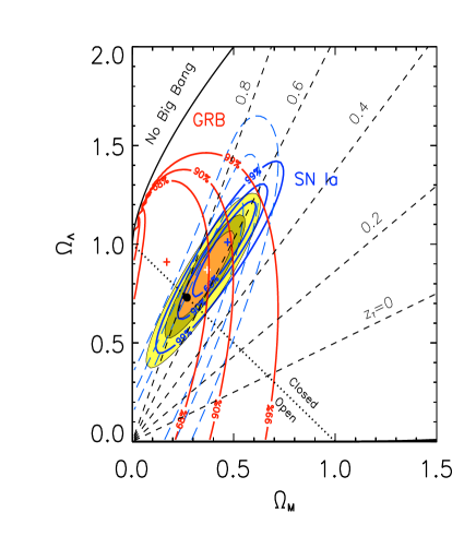
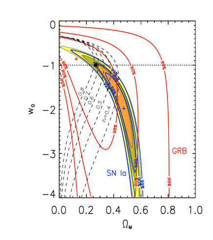
Figure 2: Left: Constraints in the $\Omega_{\rm M}$–$\Omega_{\Lambda}$ plane derived from our GRB sample (15 objects, red contours), from the “Gold” SN Ia sample (156 objects; blue solid lines, derived assuming a fixed value of $H_{0}=65$ km s^-1 Mpc^-1, making these contours slightly different from Fig. 8 of [15], and from the subset of SNe Ia at $z>0.9$ (14 objects, blue long dashed lines). The three colored ellipses are the confidence regions (orange: 68%; light green: 90%; yellow: 99%) for the combined fit of type Ia SN+GRB samples. Dashed lines correspond to the changing sign of the cosmic acceleration [i.e. $q(z)=0$] at different redshifts, as labelled. Crosses are the centers of the corresponding contours (red: GRBs; blue: SNe Ia, white: GRB+SN Ia). The black dot marks the $\Lambda$CDM cosmology. The dotted line corresponds to the statefinder parameter $r=1$ (see e.g. [16]), in this case it coincides with the flatness condition. Right: Constraints on $w_{0}$ and $\Omega_{\rm M}$ for a flat cosmology with dark energy whose equation of state is constant ($w_{0}=-1$ corresponds to a cosmological constant). Colored regions: combined (GRB+SN Ia) constraints (color code as in Fig. 2). Dashed lines correspond to the changing sign of the cosmic acceleration [i.e. $q(z)=0$] at different redshifts, as labelled. Crosses are the centers of the SNe Ia contours (blue: SNe Ia alone, white: GRB+SN Ia). The black dot marks the $\Lambda$CDM cosmology. The dotted line corresponds to the statefinder $r=1$. From [7].

To find constraints on $w_{0}$ and $w^{\prime}$ the approaches are the same as discussed above, but bearing in mind that the paucity of data, at present, does not allow to constrain more than two parameters, hence in these cases one assumes a flat universe and $w^{\prime}=0$ (and derives constraints on $\Omega_{\Lambda}$ and $w_{0}$), or the concordance model (to constrain $w_{0}$ and $w^{\prime}$).

4 Cosmological constraints

In Fig. 2 we show the results taken from Firmani et al. (2005). On the left we show the confidence contours on $\Omega_{\rm M}$, $\Omega_{\Lambda}$ when considering the GRB sample alone (15 objects, red lines), SN Ia alone (156 objects, blue lines) and the combined GRB+SN Ia sample (colored regions). The 68% confidence contours of the 15 GRBs are less restrictive than the corresponding SN Ia contours, but note that the contours of the combined sample are now consistent with the concordance model ($\Omega_{\rm M}$=0.3, $\Omega_{\Lambda}$=0.7) within the 68% level, whereas the SN Ia alone are not. The dashed blue lines are the contours corresponding to the 14 SN Ia with $z>0.9$. While the extents of the confidence contour regions are comparable (the slightly larger errors of GRBs are compensated by their larger redshifts), the inclination of these “ellipses” is different, and this is due to the different average redshifts of GRBs and this subsample of SN Ia, as explained below. The right panel of Fig. 2 shows the constraints in the $\Omega_{\rm M}$–$w_{0}$ plane, once a flat universe is assumed. Again, note that the GRBs alone do not yet compete with SN Ia, yet the constraints of the combined sample makes the concordance model ($w_{0}=-1$) more consistent, being now fully within the 68% contour levels.

5 The Cosmic Whirl

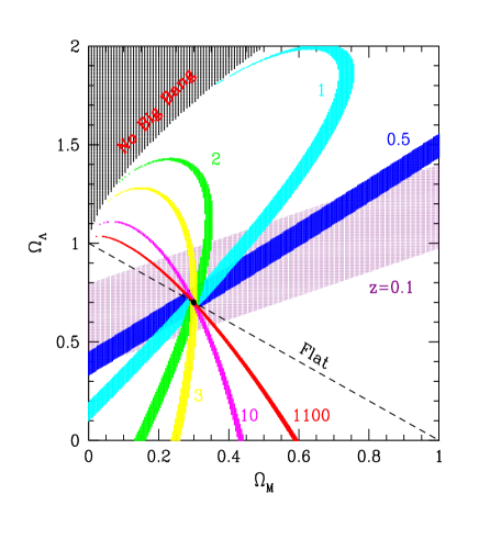
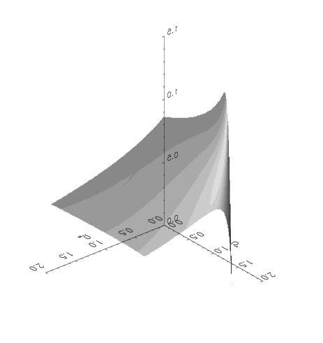
Figure 3: Left: The Cosmic Whirl. Each stripe represents the loci of points of luminosity distance differing at most by 1% to the value calculated for $\Omega_{\rm M}$=0.3, $\Omega_{\Lambda}$=0.7, for different values of the redshift, as labelled. Right: The surface of equal luminosity distance calculated for $z=1$.

It is instructive to see the behaviour of the luminosity distance $d_{\rm L}(z,\Omega_{\rm M},\Omega_{\Lambda})$ in the $\Omega_{\rm M}$– $\Omega_{\Lambda}$ plane, for different redshifts. To this aim, we show in Fig. 3 the “stripes” within which $d_{\rm L}$ changes by 1% in the $\Omega_{\rm M}$– $\Omega_{\Lambda}$ plane, for different redshift, assuming that each stripe passes through $\Omega_{\rm M}$=0.3 and $\Omega_{\Lambda}$=0.7. Note the following:

• The width of the stripes decreases for larger redshifts. This is a consequence of the topology of the surfaces of constant $d_{\rm L}$: at low redshift the surface is a gently tilted plane, at high redshifts the surface is more warped, and there appears a “mountain” with the peak close to $\Omega_{\rm M}$$\sim 0.1$ and $\Omega_{\Lambda}$$\sim 1$. This is shown in Fig. 3 for $z=1$.

• As a consequence, the “stripes” at high redshifts are curved, and at very high redshift they surround the “mountain peak”.

• Note that the width of the stripes at high redshifts become narrower for large $\Omega_{\Lambda}$–values, as a consequence of the increasing slope of the $d_{\rm L}$ plane.

This example shows that if we have a sample of standard candles characterized by a small range in redshifts, the corresponding confidence contours in the $\Omega_{\rm M}$– $\Omega_{\Lambda}$ plane will be elongated in the the direction of the stripe of the average redshift of the sample. This easily explains why the confidence contours derived by using SN Ia are elongated in the direction of the $d_{\rm L}(z\sim 0.5)$ stripe, while the contours derived by the WMAP satellite are elongated along $d_{\rm L}(z\sim 1100)$ stripe. The contours derived using our GRB sample, of larger average redshift than SN Ia, are more vertically elongated. Therefore there is a counterclockwise rotation of the confidence contours when increasing the average redshift of the standard candles we are using: only a class of sources spanning a large range of redshifts can give an accurate value of $\Omega_{\rm M}$ and $\Omega_{\Lambda}$.

6 The future

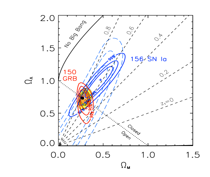
Figure 4: Contours levels in the $\Omega_{\rm M}$, $\Omega_{\Lambda}$plane for a simulation of 150 GRBs, according to method 4 (see text and compare with Fig. 2 showing the results with the current sample of 15 GRBs). Blue solid lines are the contours for the 156 SN Ia of the gold sample of [15], blue dashed lines correspond to the subsample of high–$z$ SN Ia, colored regions correspond to the combined sample of 156 SN Ia and the 150 GRBs. The blue cross is the position of the minimum $\chi^{2}$ for SN Ia only, the red and white crosses are the positions of the minimum $\chi^{2}$ for GRB only and the combined GRB+SN Ia sample, respectively. These crosses are partially hidden by the black dot, marking the $\Omega_{\rm M}$=0.3, $\Omega_{\Lambda}$=0.7 point. Black dashed lines correspond to the changing sign of the cosmic acceleration [i.e. $q(z)=0$] at different redshifts, as labelled.

The constraints posed by WMAP ([17]) and SN Ia ([15], [12]), together with cluster of galaxies ([1]) have convincingly led towards the so called “concordance cosmological model”, a flat universe with $\Omega_{\rm M}$=0.73  and $\Omega_{\Lambda}$=0.27. So, why bother? We care because even if we pretend to know how the universe is now, we do not know how it was. This ignorance is one of the obstacles towards the understanding of what is the dark energy. And this is indeed one of the most important and fascinating challenges of modern (astro)physics. This is why GRBs can be extremely important, because they can bridge the gap between relatively close–by supernovae and the fluctuations of the cosmic microwave background. They may not be the only tool, since also through the integrated Sach–Wolfe effect one hopes to learn how the universe was in the past. But having more than one way to measure the universe is certainly not redundant, since each way brings its own uncertainties, selection effects and so on. Furthermore, we have ahead a few years of SWIFT results, which will hopefully discover a few hundreds of new bursts with well measured properties, especially their afterglows at early times, which will greatly improve the now poor sample of 15 cosmologically useful GRBs. The fact that the measured fluences do not strongly correlate with redshifts (see GGL) means that even for high redshifts GRBs we can well determine the fluence itself and the spectral parameters of the prompt emission (i.e. $E_{\rm peak}$). SWIFT itself will follow the early afterglow with unprecedented accuracy, and this will certainly help to construct detailed lightcurves (in X–rays and in the optical) allowing to pinpoint the jet break time more accurately. For bursts at $z>5$, therefore in the absence of the optical lightcurve (the optical flux is strongly absorbed by Lyman $\alpha$ absorption) one can derive the jet break time from the X–ray and the infrared lightcurves, and in this case robotic IR telescopes like REM (for the early data, [18]), and larger telescopes (for later data) will help. Fig. 4 shows how the constraints on the cosmological parameters could improve passing from 15 to 150 bursts, a number comparable to the current SN Ia gold sample of [15] which will be hopefully reached after 2–3 years of SWIFT. This simulation has been performed (Lazzati et al. in preparation) assuming a “luminosity function” of $E_{\rm iso}$ and an appropriate redshift distribution (see, e.g. [14]). We have assigned relative errors of 20% on $t_{\rm break}$, 16% on $E_{\rm peak}$ and 10% on the fluence (these are the average relative errors for the 15 GRBs). The average redshift of the simulated sample is $\langle z\rangle\sim 2.26$. This is the reason of the inclination of the ellipses of the contour levels (cfr. Fig. 3).

The results shown in Fig. 4 suggest that GRBs, reaching larger redshifts than SN Ia, can constrain $\Omega_{\rm M}$, $\Omega_{\Lambda}$ better than SN Ia. Even tighter constraints can be achieved, of course, after a sufficient number of GRBs are observed at small redshifts, allowing a cosmology–independent calibration of the Ghirlanda relation, and/or after a robust theoretical interpretation is found for this relation.

For an on–line update: www.merate.mi.astro.it/$\sim$ghirla/deep/blink.htm.

- [1] \BYAllen, S.W., Schmidt, R.W., Ebeling, H., Fabian, A.C., & van Speybroeck, L. \INMNRAS3532004457
- [2] \BYBarkana, R. & Loeb, A. \INApJ601200464
- [3] \BYBloom, J.S., Frail, D.A. & Kulkarni, S.R. \INApJ5942003674
- [4] \BYDai, Z.G., Liang, E.W. & Xu, D. \INApJ2004
- [5] \BYFrail, D.A., Kulkarni, S.R., Sari, R. et al. \INApJ5622001L55
- [6] \BYFirmani, C., Avila–Reese, V., Ghisellini, G. & Tutukov, A.V. \INApJ61120041033
- [7] \BYFirmani, C., Ghisellini, G., Ghirlanda, G. & Avila–Reese, V. \INMNRAS (Letters)2005, in press (astro–ph/0502186)
- [8] \BYGhirlanda, G., Ghisellini, G. & Lazzati, D. \INApJ6162004a331 (GGL)
- [9] \BYGhirlanda, G., Ghisellini, G., Lazzati, D. & Firmani, C. \INApJ6132004bL13 (GGLF)
- [10] \BYGhirlanda, G., Ghisellini, G. & Firmani, C. \INsubm. to MNRAS2005 (astro–ph/0502186)
- [11] \BYLamb, D.Q. & Reichart, D.E. \INGRBs in the afterglow era, Eds. E. Costa, F. Frontera, J. Hjorth, Berlin Heidelberg: Springer2001226
- [12] \BYPerlmutter, S. et al. \INApJ5171999565
- [13] \BYPhyllips, M.M. \INApJ4131993L105
- [14] \BYPorciani, C. & Madau, P. \INApJ5482001522
- [15] \BYRiess, A. G., Strolger, L–G., Tonry H., et al. \INApJ6072004665
- [16] \BYSahni, V. \INpreprint2004astro–ph/0403324
- [17] \BYSpergel, D.N., Verde, L., Peiris, H.V., et al. \INApJS1482003175
- [18] \BYZerbi, F., et al. \INAstron. Nachriten32220015