Cosmological Three-Point Function:
Testing The Halo Model Against Simulations

Abstract

We perform detailed comparison of the semi-analytic halo model predictions with measurements in numerical simulations of the two and three point correlation functions (3PCF), as well as power spectrum and bispectrum. We discuss the accuracy and self-consistency of the halo model description of gravitational clustering in the non-linear regime and constrain halo model parameters. We exploit the recently proposed multipole expansion of three point statistics that expresses rotation invariance in the most natural way. This not only offers technical advantages by reducing the integrals required for the halo model predictions, but amounts to a convenient way of compressing the information contained in the 3PCF. We find that, with an appropriate choice of the halo boundary and mass function cut-off, halo model predictions are in good agreement with the bispectrum measured in numerical simulations. However, the halo model predicts less than the observed configuration dependence of the 3PCF on $\sim$ Mpc scales. This effect is mainly due to quadrupole moment deficit, possibly related to the assumption of spherical halo geometry. Our analysis shows that using its harmonic decomposition, the full configuration dependence of the 3PCF in the non-linear regime can be compressed into just a few numbers, the lowest multipoles. Moreover, these multipoles are closely related to the highest signal to noise eigenmodes of the 3PCF. Therefore this estimator may simplify future analyses aimed at constraining cosmological and halo model parameters from observational data.

1 Introduction

Galaxy formation and evolution still lacks a compelling explanation from first principles. In the absence of a successful theory, galaxy clustering can be described assuming that galaxies are biased tracers of the underlying dark matter distribution. Recently, the halo model for gravitational clustering (Neyman & Scott, 1952; Peebles, 1974; McClelland & Silk, 1977a, b, 1978) has been revived in cosmology as an attempt to provide an accurate picture of gravitational clustering in the non-linear regime as seen by high-resolution N-body simulations (Scherrer & Bertschinger, 1991; Sheth & Jain, 1997; Seljak, 2000; Ma & Fry, 2000a, b; Scoccimarro et al., 2001; Cooray & Hu, 2001).

Halo model provides a simple prescription for the analytic computation of N-point correlation functions which are the most widely used statistics for gravitational clustering (see Cooray & Sheth (2002) and references therein). In particular, Seljak (2000) suggested that the power spectrum of dark matter and galaxies are consistent with this approach, whereas Peacock & Smith (2000) reached similar conclusions using mock catalogs. Ma & Fry (2000a, b) derived predictions for the power spectrum, bispectrum and its Fourier counterparts, the two and three-point correlation functions, that were found to be in agreement with numerical simulations. Scoccimarro et al. (2001) (hereafter SSHJ), discussed the halo model predictions for the power spectrum, and bispectrum, as well as the higher-order cumulants, $S_{p}$, and concluded that dark matter clustering in the halo model is in good agreement with measurements from N-body simulations on large scales ($\rm{r}>1\rm{Mpc/h}$). However, the agreement was at the 20 % level only on smaller scales ($\rm{r}\lower 2.15277pt\hbox{$\;\buildrel<\over{\sim}\;$}1\rm{Mpc/h}$). They also showed a first comparison with the variance from APM galaxies.

Progress on numerical simulations has triggered a number of theoretical developments in the halo model. New elements such as substructure (see e.g.,  Sheth, 2003; Sheth & Jain, 2003; Dolney et al., 2004) and halo geometry (Jing & Suto, 2002) have been recently incorporated into the model to provide a more realistic description of dark matter clustering. Other developments have focused on describing galaxy bias using the so-called halo occupation distribution, a prescription of filling halos with galaxies in a stochastic fashion (Berlind & Weinberg, 2002; Berlind et al., 2003; Zehavi et al., 2004).

Recently, Takada & Jain (2003a) have thoroughly explored halo model predictions for the three-point correlation function (3PCF hereafter) of dark matter and galaxies. They concluded that halo model predictions for the dark matter described adequately only certain triangle configurations. They fail to match simulations for triangles with side length $\rm{r}\approx~{}1\rm{Mpc/h}$. Wang et al. (2004) investigated the two- and three-point functions and compared analytic results to dark matter simulations and galaxy clustering observations from the 2dF. They claim their predictions closely reproduce numerical results and observations.

In this paper we focus on the dark matter three-point correlation functions in real and Fourier space. In particular, our principal aim is to carry out a detailed comparison of halo model predictions with measurements in high resolution simulations to test the validity of the model and constrain halo model parameters.

The present analysis differs from previous work in the literature in several ways:

• We present new technology to perform the necessary integrals using multipole expansion, in particular the dimension of the integrals is significantly reduced in our prescription.

• For the first time, we test the validity of the halo model against N-body simulations simultaneously in real and Fourier space, at the two and three-point level.

• We constrain halo parameters in a self-consistent fashion: all statistics are predicted from halo model parameters. In particular, we do not use the Smith et al. (2003) as an ingredient of the model, which has become common usage when constraining bias from observational data (see e.g.,  Zehavi et al., 2004; Wang et al., 2004). We show that using the halo model in a self-consistent way provides a good fit to N-body simulations, provided one leaves the halo boundary as a free parameter, and large-mass haloes, not present in simulations, are removed from the mass function accordingly.

• We extend our analysis for the recently proposed multipole expansion of three-point statistics, which expresses rotation invariance naturally. This allows the compression three-point statistics into a few multipoles even in the non-linear regime. This is especially convenient for constraining non-Gaussianity from gravitational clustering.

2 Halo Model

According to the halo model picture, the non-linearly evolved dark matter distribution is described in terms of the clustering properties dark haloes, quasi-equilibrium objects formed by gravitational collapse, (see Cooray & Sheth, 2002, for a review and references therein). In this context, correlation functions are decomposed into contributions arising from correlations among particles inhabiting dark-matter haloes. For convenience throughout this paper we shall closely follow SSHJ to describe the statistics of gravitational clustering within the halo model.

2.1 Halo profile

Numerical simulations suggest that dark haloes have a universal profile (Navarro et al., 1997; Moore et al., 1998). Here we shall adopt the NFW profile,

$$\rho(r)=\frac{f}{4\pi}{\left(\frac{c}{{R_{v}}}\right)}^{3}\frac{1}{cr/{R_{v}}(1+cr/{R_{v}})}$$ (1)

and its Fourier transform, $\rho(k)=\int_{0}^{R_{v}}4\pi r^{2}dr\rho(r)j_{0}(kr)$, where $j_{0}(x)=\sin x/x$ is the zeroth-order spherical Bessel function, takes the form (see SSHJ),

$$\rho(k,y)=f\left[\sin\eta~{}\{\rm{Si}[\eta(1+c)]-\rm{Si}(\eta)\}+\cos\eta~{}\{\rm{Ci}[\eta(1+c)]-\rm{Ci}(\eta)\}-\frac{\sin(\eta c)}{\eta(1+c)}\right]$$ (2)

with $f=1/\left[\ln(1+c)-c/(1+c)\right]$, $\eta=k{R_{v}}/c$, $c$ is the concentration parameter, and $\rm{Si}$ and $\rm{Ci}$ are the sine and cosine integral functions. The virial radius, ${R_{v}}$, is the characteristic scale which separates the inner $\rm{r}^{-1}$ from the outer $\rm{r}^{-3}$ behavior of the profile. Above we have assumed that the halo profile is truncated at ${R_{v}}$, an assumption that shall be relaxed in order to match clustering measurements in N-body simulations (see §4). The concentration parameter is not well constrained from simulations and we adopt the standard halo parametrization with halo mass

$$c(M)=c_{0}\left(\frac{M}{M_{*}}\right)^{-\beta}$$ (3)

$M_{*}$ sets the non-linearity scale $\sigma(M_{*})=\delta_{c}$, being $\sigma$ the linear rms mass fluctuation and $\delta_{c}=1.686$ is the linear overdensity required for spherical collapse. We shall assume the values suggested by numerical simulations $c_{0}=9$, $\beta=0.13$ Bullock et al. (2001), but have checked that changing halo concentration parameters by as much as 50 % does not affect significantly our predictions within the range of scales probed by our simulations.

2.2 Halo mass function

A basic ingredient of the halo model is the mass function, $n(M)$, which describes how many objects of mass in the range $M$ and $M+dM$ end up collapsing to form bound structures. Here we use the extension of the Press-Schechter formalism provided by Sheth & Tormen (1999) that accurately describes N-body results (Jenkins et al., 2001):

$$n(M)MdM=\bar{\rho}\frac{dy}{y}n(\nu)=\bar{\rho}\frac{dy}{y}A~{}\gamma\sqrt{\frac{g(\nu)}{2\pi}}\left(1+g(\nu)^{-p}\right)\exp(-g(\nu)/2)$$ (4)

with $\gamma=d\ln\sigma^{2}/d\ln R$, $g(\nu)=\alpha\nu^{2}$, $\alpha=0.707$, $\nu=\delta_{c}/\sigma$, $A=0.322$, $p=0.3$, $y=(R/R_{*})=(M/M_{*})^{1/3}$, $R$ is the lagrangian radius, and $R_{*}={R_{v}}~{}\Delta$ is the non-linear (lagrangian) scale, where $\Delta=200,340$ for $\Omega_{m}=1,0.3$ cosmologies, respectively.

2.3 Halo clustering

Halo correlations can be included in the model by assuming a biasing prescription between the halo and the underlying mass distribution. We follow the approach introduced by Mo & White (1996) in the context of the spherical collapse model, and adopt the fitting formula given by Sheth & Tormen (1999):

$$b(\nu)=1+\frac{g(\nu)-1}{\delta_{c}}+\frac{2p}{\delta_{c}(1+g(\nu)^{p})}$$ (5)

and we neglect quadratic and higher-order biasing terms. We note that a non-vanishing quadratic bias only affects the three-point statistics (or higher orders) on large scales and we have checked that its contribution is a few per cent at most.

3 Halo Model Statistics

Halo model statistics are particularly simple to formulate in Fourier space. Complications arising from convolutions of halo profiles become simple products in transform space.

According to the halo model approach, the non-linear power spectrum of the mass fluctuations is the result of two independent contributions: one coming from the single halo profile auto-correlation that dominates on small-scales and another one given by the correlation among dark matter particles in different halos that accounts for the large-scale clustering. This way we can write,

$$P(k)=\left[I_{11}(k)\right]^{2}~{}P_{L}(k)+I_{02}(k,k)$$ (6)

where,

$$I_{ij}(k_{1},\cdots,k_{j})=\int\frac{dy}{y}n(y)b_{i}(y)\left[\rho(k_{1},y)\cdots\rho(k_{j},y)\right]{\left(\frac{R^{3}_{*}y^{3}}{6\pi^{2}}\right)}^{j-1}$$ (7)

where $b_{0}=1$, $b1=b(\nu)$, and $b_{i}=0$ for $i>1$ as we neglect quadratic and higher-order biasing terms, and $P_{L}(k)$ is the linear power spectrum, for which we assume the Bond & Efstathiou (1984) parametrization. The two-point correlation function follows by Fourier transforming $P(k)$,

$$\xi(r)=\int\frac{k^{2}}{2\pi^{2}}dk~{}P(k)~{}j_{0}(kr)$$ (8)

where $j_{0}$ is the zero-order spherical Bessel function.

The bispectrum, $B_{123}\equiv B(k_{1},k_{2},k_{3})$, can be expressed as a sum of three-point correlations among mass particles residing in one, two, and three haloes, respectively:

$$B_{123}=\left[\prod_{i=1}^{3}I_{11}(k_{i})\right]B^{PT}_{123}+\{I_{11}(k_{1})I_{12}(k_{2},k_{3})P_{L}(k_{1})+{\rm perm(1,2,3)}\}+I_{03}(k_{1},k_{2},k_{3})$$ (9)

where $B^{PT}$ denotes the bispectrum from second order Perturbation Theory (PT). By design, halo model recovers weakly non-linear theory predictions on large scales, since $k\rightarrow 0$, $I_{11}\approx 1$ and $I_{12},I_{02},I_{03}\approx 0$, or equivalently, $P\approx P_{L}$, $B_{123}\approx B^{PT}$.

The 3PCF is a triple Fourier transform of the bispectrum,

$$\zeta(r_{1},r_{2},r_{3})=\int\prod_{i=1}^{3}d^{3}{\bf k}_{i}~{}B_{123}~{}e^{i({\bf k}_{1}\cdot{\bf r}_{1}+{\bf k}_{2}\cdot{\bf r}_{2}+{\bf k}_{3}\cdot{\bf r}_{3})}\delta_{Dirac}({\bf k}_{1}+{\bf k}_{2}+{\bf k}_{3}).$$ (10)

In the context of halo models, $\zeta$ is a complex object: Takada & Jain (2003a) have shown that the evaluation of the two- and three-halo terms in real space involves eight- and twelve-dimensional integrals, respectively; this is untractable. They reduce the dimensionality of the integrals to two by switching to Fourier-space and taking a number of approximations in the corresponding kernels.

Our approach is significantly different in that, although we also use Fourier-space formalism, we further decompose correlation functions into harmonic multipoles. This greatly simplifies the exact analytic expressions, therefore we do not need to take the approximations used by Takada & Jain (2003a) for the 2- and 3-halo terms. We note that, for the 1-halo term, their estimator is expressed as a four dimensional integration and it is exact. The only approximation we take is that we use a finite number of multipoles. We will see that this is an excellent approximation, except for degenerate (isosceles) triangles, where the amplitude of the harmonic coefficients decrease slowly with multipole order. In our formalism, the 3PCF can be expressed as a two-dimensional Hankel transform of the bispectrum, for each harmonic multipole (Szapudi, 2004):

$$\zeta(r_{1},r_{2},\theta)=\sum_{\ell}\frac{2\ell+1}{4\pi}\zeta_{\ell}(r_{1},r_{2})~{}P_{\ell}(\cos\theta)$$ (11)

where $\theta$ is the angle between ${\bf{r_{1}}}$ and ${\bf{r_{2}}}$, $P_{\ell}$ is the legendre polynomial of order $\ell$, $\zeta_{\ell}(r_{1},r_{2})$ is the harmonic 3PCF,

$$\zeta_{\ell}(r_{1},r_{2})=\int dk_{1}~{}dk_{2}\frac{k_{1}^{2}}{2\pi^{2}}\frac{k_{2}^{2}}{2\pi^{2}}(-1)^{\ell}~{}B_{\ell}(k_{1},k_{2})j_{\ell}(k_{1}r_{1})j_{\ell}(k_{2}r_{2})$$ (12)

and $B_{\ell}$ is the Legendre transform of the bispectrum,

$$B_{\ell}(k_{1},k_{2})=2\pi\int_{-1}^{1}d(\cos\theta)~{}B(k_{1},k_{2},\theta)~{}P_{\ell}(\cos\theta)\ .$$ (13)

High multipoles ($\ell\gg 1$), only important for the isosceles triangles, can be easily computed employing the large-$\ell$ limit of spherical Bessel functions, $j_{\ell}(x)\approx\sqrt{\pi/(2\ell+1)}~{}\delta_{Dirac}(\ell+1/2-x)$,

$$\zeta_{\ell}(r_{1},r_{2})=\left(\frac{L}{2\pi}\right)^{3}\frac{1}{(r_{1}r_{2})^{3}}(-1)^{\ell}B_{\ell}\left(\frac{L}{r_{1}},\frac{L}{r_{2}}\right)$$ (14)

where $L\equiv\ell+1/2$. It is convenient to define the reduced (or hierarchical) 3PCF,

$$Q(r_{1},r_{2},r_{3})=\frac{\zeta(r_{1},r_{2},r_{3})}{\xi(r_{1})\xi(r_{2})+\xi(r_{2})\xi(r_{3})+\xi(r_{3})\xi(r_{1})}$$ (15)

and similarly, the reduced bispectrum in Fourier space,

$$Q(k_{1},k_{2},k_{3})=\frac{B_{123}}{{P(k_{1})P(k_{2})+P(k_{2})P(k_{3})+P(k_{3})P(k_{1})}}.$$ (16)

PT and the stable clustering hypothesis predict them to be weakly dependent of scale in the quasi-linear and non-linear regimes, respectively. Similar to eq(13), it is convenient to decompose the reduced 3PCF, $Q(r_{1},r_{2},r_{3})$, in its harmonic multipoles by taking its Legendre transform,

$$Q_{\ell}(r_{1},r_{2})=2\pi\int_{-1}^{1}d(\cos\theta)~{}Q(r_{1},r_{2},\theta)~{}P_{\ell}(\cos\theta)$$ (17)

where $\theta$ is the angle between ${\bf r_{1}}$ and ${\bf r_{2}}$. Analogous expressions can be written for the harmonic multipoles of the reduced bispectrum.

Since the bispectrum itself is obtained by performing a one-dimensional integration of the halo correlations over the mass function, in order to compute the three-point function multipoles $\zeta_{\ell}$, as given by eq(12), four-dimensional integrals are required for each $\ell$ . Figure 1 shows how the 3PCF in the non-linear regime can be efficiently reconstructed from its lowest harmonic multipoles. In particular, for the isosceles triangle with side length $r=1~{}\rm{Mpc/h}$, only three harmonics contribute significantly to the 3PCF. The monopole essentially determines the amplitude, the (negative) quadrupole and, to a lesser extent, the octopole shape the configuration dependence (see top left and middle panels). Thus the full configuration dependence of the 3PCF can be reconstructed from these three harmonics (see top right panel) to an excellent approximation. Only collinear configurations, $\theta=0,\pi$ have (increasingly smaller) contributions from higher order terms. Similarly, the triangles with $r_{1}=2~{}\rm{Mpc/h}$, and $r_{2}=6~{}\rm{Mpc/h}$ are shaped by the quadrupole and therefore, the configuration dependence is encoded in this single harmonic to a large extent (see lower panels). These examples are typical for all non-degenerate triangles we have checked.

As we shall show below (see §4), in general, only the lowest multipoles are non-zero and thus full configuration dependence of the non-linear cosmological 3PCF can be compressed in a few numbers. Thus using the multipole expansion greatly reduces the problem of constraining non-gaussianity from gravitational clustering.

4 Comparison to Numerical Simulations

We have used two sets of $\Lambda$CDM simulations from the public Virgo simulation archive with cosmological parameters $\Omega_{0}=0.3$, $\Omega_{\Lambda}=0.7$, $h=0.7$, $\Gamma=0.21$ and $\sigma_{8}=0.9$ and no baryons. The original Virgo simulation has $256^{3}$ particles in a box-size of $L=239.5h^{-1}$Mpc, mass resolution of $6.86\cdot 10^{10}h^{-1}M_{\sun}$ and softening length $L_{soft}=25h^{-1}$kpc, and a larger box (VLS) simulation $L=479h^{-1}$Mpc that contains $512^{3}$ particles, same mass resolution than the original Virgo simulation and $L_{soft}=30h^{-1}$kpc . These simulations have been gravitationally evolved using a P3M code (Macfarland et al., 1998; Couchman et al., 1995).

Bispectrum is computed through FFT’s on $256^{3}$ grid-points with the method of Scoccimarro et al. (1998) (see their Appendix A). The 3PCF is measured with the fast algorithm based on multi-resolution KD-trees of Moore et al. (2001) and Gray et al. (2004) using the estimator of Szapudi & Szalay (1998). Limited by computational resources, we dilute simulations to 10 percent for the 3PCF at scales $\rm{r}\lower 2.15277pt\hbox{$\;\buildrel<\over{\sim}\;$}2~{}\rm{Mpc/h}$ and at 1 percent at larger scales. For these computations the number of points in auxiliary random sets are roughly 10 times larger than those of diluted simulation data sets. The large box simulation is cut into eight independent sub-volumes (octants) of half box size and measured separately. Mean values are obtained by averaging these eight sub-volumes and the orginal Virgo simulation. Errorbars are simply computed from the dispersion over sub-volumes. We note that this error estimate might underestimate true errors since sub-volumes are somewhat correlated. However, for the small scales analyzed in this paper, our sub-samples are effectively independent.

Our approach is to discuss halo model predictions for a fiducial model that provides a good fit to the 2-point statistics (i.e. power spectrum and 2PCF) measured in the simulations. Then we explore systematically the ability of such a model of describing 3-point statistics in N-body experiments. We set cosmological parameters to match those of our simulations and the halo concentration parameter is set to $c_{0}=9$ and $\beta=0.13$ in eq(3), as in SSHJ. We have verified that changing the amplitude and slope of the concentration parameter within a reasonable range (i.e. by a factor $\sim 2$) has a negligible effect on the 2PCF and 3PCF for $k\lower 2.15277pt\hbox{$\;\buildrel<\over{\sim}\;$}10$, or ${\rm{r}}\lower 2.15277pt\hbox{$\;\buildrel>\over{\sim}\;$}0.2\rm{Mpc/h}$ (see also Fig.2 in Takada & Jain, 2003a), therefore we fix this parameter to its fiducial values to simplify further studies.

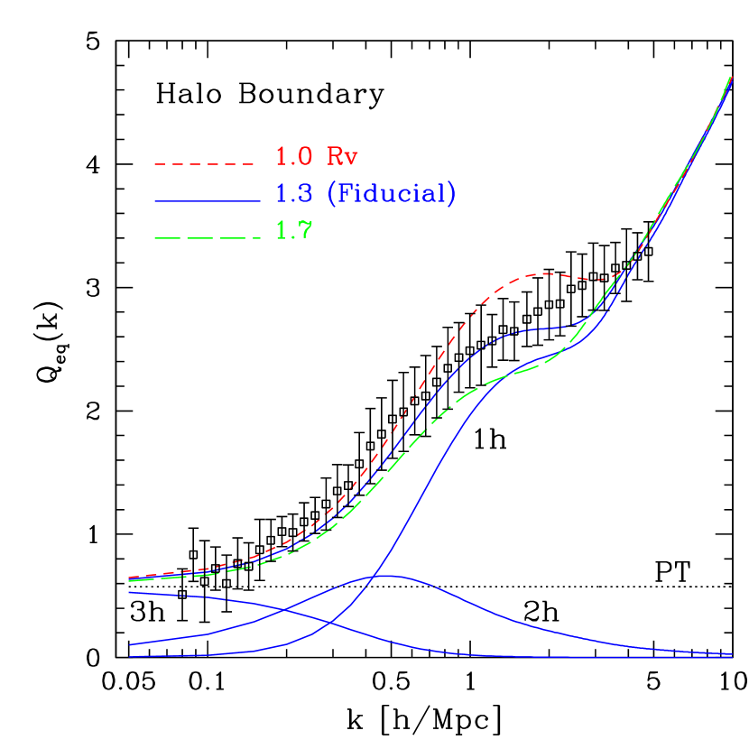
Figure 5: Halo boundary effect on the reduced bispectrum for equilateral triangles $Q_{eq}(r)$. $Q_{eq}(r)$ is very sensitive to changes in the halo boundary: larger boundaries enhance more the denominator (that depends on the 2PCF) than the 3PCF, what results in a significant drop of the reduced bispectrum on non-linear scales. On large-scales PT holds (see dotted line). Note that the fiducial model matches simulations, but exhibits a bump on $k\approx 1-2\rm{h/Mpc}$, that is not seen in N-body results.

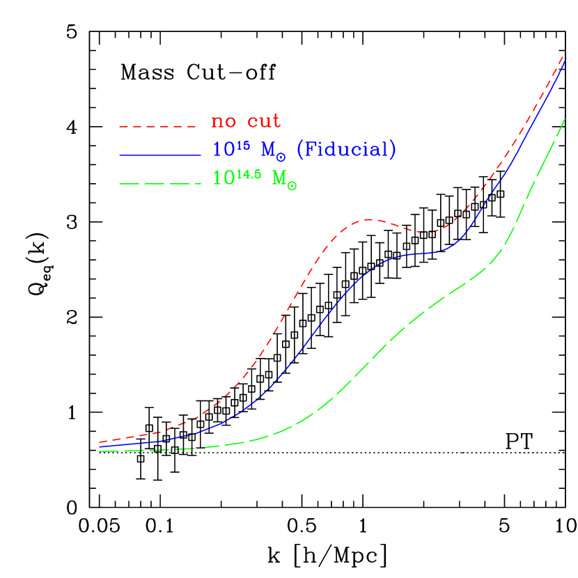
Figure 6: Same as Fig.5, but for the mass cut-off. Excluding the largest mass haloes significantly lowers the amplitude of the reduced bispectrum.

Basic halo model parameters yield a 2PCF that does not fit well our N-body results. This is clearly seen in Figs.2-6, especially for scales, $\rm{r}\approx 1~{}\rm{Mpc/h}$. To improve the precision, we introduce standard “tweaks” of the basic set of ingredients of the model. The assumption that the halo boundary (the radius up to which halo mass is encompassed) is exactly given by the virial radius is in fact quite arbitrary. Treating this as an additional free parameter to the 1-halo terms in the 2PCF and 3PCF improves the transition scales, $0.5-5~{}\rm{Mpc/h}$, between linear (or quasi-linear) to fully non-linear scales (see Figs.2 and 5). Fig.5 shows that a halo boundary beyond the virial radius increases the 2PCF on small scales and reduces the “bump” in the reduced bispectrum for equilateral triangles $Q_{eq}(k)$. Setting the boundary to the fiducial value, $1.3{R_{v}}$, yields good agreement both with the 2PCF and 3PCF in simulations. In particular, for the 2PCF, the agreement with N-body is comparable to the fitting function provided by Smith et al.(2003). However, on large scales, halo model tends to slightly overpredict simulations, whereas Smith et al. slightly underpredicts them. Similarly, Fig.4 shows that our fiducial model provides a good fit to the matter power spectrum measured in our N-body simulations.

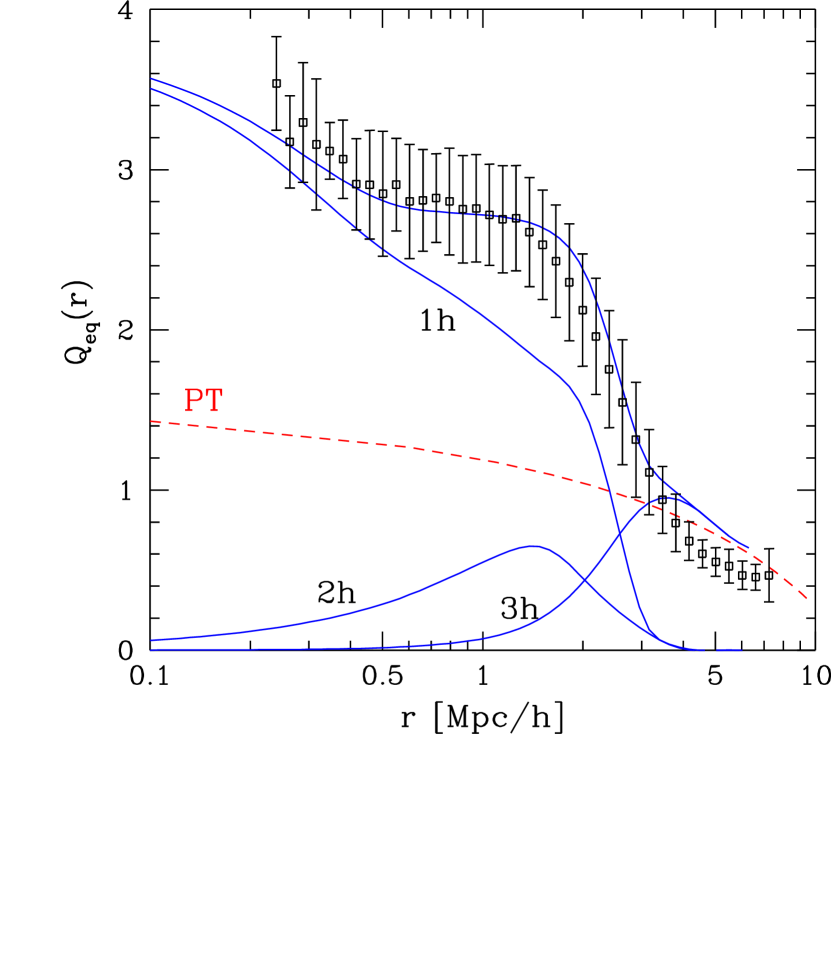
Figure 8: Reduced 3PCF for equilateral triangles: the fiducial halo model (upper solid line) shows good agreement with simulations. The small-scale enhancement is determined by the one-halo term, while the amplitude on the transition scales $\rm{r}\approx 1-3~{}\rm{Mpc/h}$ reflects the non-trivial interplay between different halo terms (lower solid lines). The good agreement found with N-body in this range is a remarkable success of the halo model. The observed mismatch between model and simulations on larger scales is due to the model slightly overestimating the 2PCF (that goes into the denominator of $Q_{eq}$) on that range of scales (see Fig.2).

Our results are in full agreement with that of Takada & Jain (2003a) who also implemented the “exclusion effect”. This excludes correlations between haloes at distances smaller than the sum of their virial radii. Halo exclusion is an inherently real space phenomenon, and it would be difficult, if not impossible, to correctly implement in our Fourier-based approach. We have checked using approximations (which essentially cut off the two-halo term on small scales) that halo exclusion plays a subdominant role in describing the 3PCF (see also Fig.8 in Takada & Jain, 2003a).

In addition, we try to mimic the finite volume effects affecting N-body simulations by imposing a cut-off in the mass function, excluding haloes of masses $M\lower 2.15277pt\hbox{$\;\buildrel>\over{\sim}\;$}M_{cut}$. This has a critical effect on clustering on scales $\rm{r}\lower 2.15277pt\hbox{$\;\buildrel<\over{\sim}\;$}5\rm{Mpc/h}$. We find that imposing no cut-off overpredicts the clustering observed in simulations whereas excluding haloes of $\rm{M}\lower 2.15277pt\hbox{$\;\buildrel>\over{\sim}\;$}10^{14.5}\rm{M}_{\sun}$ results in too low a 2PCF. This is even more evident in the reduced bispectrum for equilateral triangles $Q_{eq}(k)$ (see Fig.5). Our fiducial value $\rm{M}_{cut}=10^{15}\rm{M}_{\sun}$ reproduces reasonably well simulation results. This behavior was already observed by SSHJ and Wang et al. (2004) who found different best-fit values for their smaller-box ($L=300\rm{Mpc/h}$) simulations. While these works did not discuss the effect of the mass cut-off on the 2PCF, we have made sure that our fiducial choice, motivated by the 3PCF, still reproduces the 2PCF accurately.

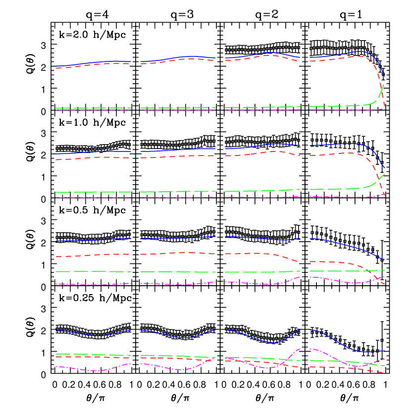
Figure 7: Reduced bispectrum for different triangle configurations. Rows show increasingly larger scales from top to bottom, while columns evolve towards more symmetric triangles from left ($q=4$) to right ($q=1$, isosceles triangle), where $q\equiv k_{2}/k_{1}$, and $k\equiv k_{1}$. Lines show the total (solid), one-halo (short-dashed), two-halo (long-dashed), and three-halo (dot-dashed) terms. Note the continuity of all the lines through plotted triangle configurations (from left to right). This “boundary condition” can be expressed as $Q(k,q,\theta/\pi=1)=Q(k,q-1,\theta/\pi=0)$, since these configurations describe the same triangle: the fact that the lines continue as expected shows the accuracy of our integration. It is seen that large scales show a more pronounced configuration dependence as dictated by the three-halo term. Triangles on small-scales are rather flat, except for the “shoulder” displayed by the isosceles triangles.

The above two extra parameters fix our fiducial model. In what follows, we shall use it to work out detailed predictions for the 3PCF and its harmonic multipoles $\zeta_{\ell}$ (see eqs(11) and (12)), and compare them to measurements N-body simulations. Fig.7 displays the reduced bispectrum for several different triangular configurations. It appears that large scales present a more pronounced configuration dependence than predicted by the three-halo term. Triangles on small-scales are rather flat, except for the “shoulder” displayed by the isosceles triangles.

Halo model prediction for the reduced 3PCF for equilateral triangles, $Q_{eq}(r)$ is in good agreement with N-body results as shown in Fig.8. On scales $\rm{r}~{}\lower 2.15277pt\hbox{$\;\buildrel>\over{\sim}\;$}3\rm{Mpc/h}$ the model slightly overpredicts simulations, similarly to the 2PCF on the same scales (see Fig.2 and Fig.3). Note that the non-linear halo model converges, albeit slowly, to the PT on large-scales.

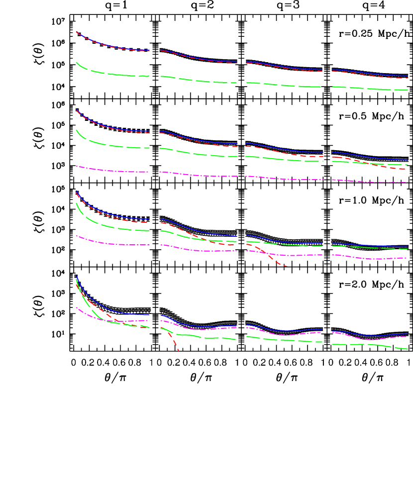
Figure 9: 3PCF for different triangle configurations: lines go as in Fig.7. Halo model predictions are shown to be in good agreement with simulations (symbols). On scales $\rm{r}\lower 2.15277pt\hbox{$\;\buildrel>\over{\sim}\;$}1~{}\rm{Mpc/h}$ the model shows a flatter configuration dependence than simulations, but they still agree within errorbars for most of the cases. Note that in real space the triangle “boundary condition” (see text and Fig.7 for details) is expressed as $\zeta(r,q,\theta/\pi=1)=\zeta(r,q+1,\theta/\pi=0)$, where $q\equiv r_{2}/r_{1}$, and $r\equiv r_{1}$.

Fig.9 displays the configuration dependence of the 3PCF for the transition scales as predicted by the halo model (lines) compared to numerical simulations (symbols). The agreement between the model and simulations is generally within the errorbars. Moreover, the rich configuration and scale dependence made up by the non-trivial interplay between different halo terms is observed in simulations. This can be considered as the best confirmation that the basic idea of halo models carries over to the three-point function without major modifications.

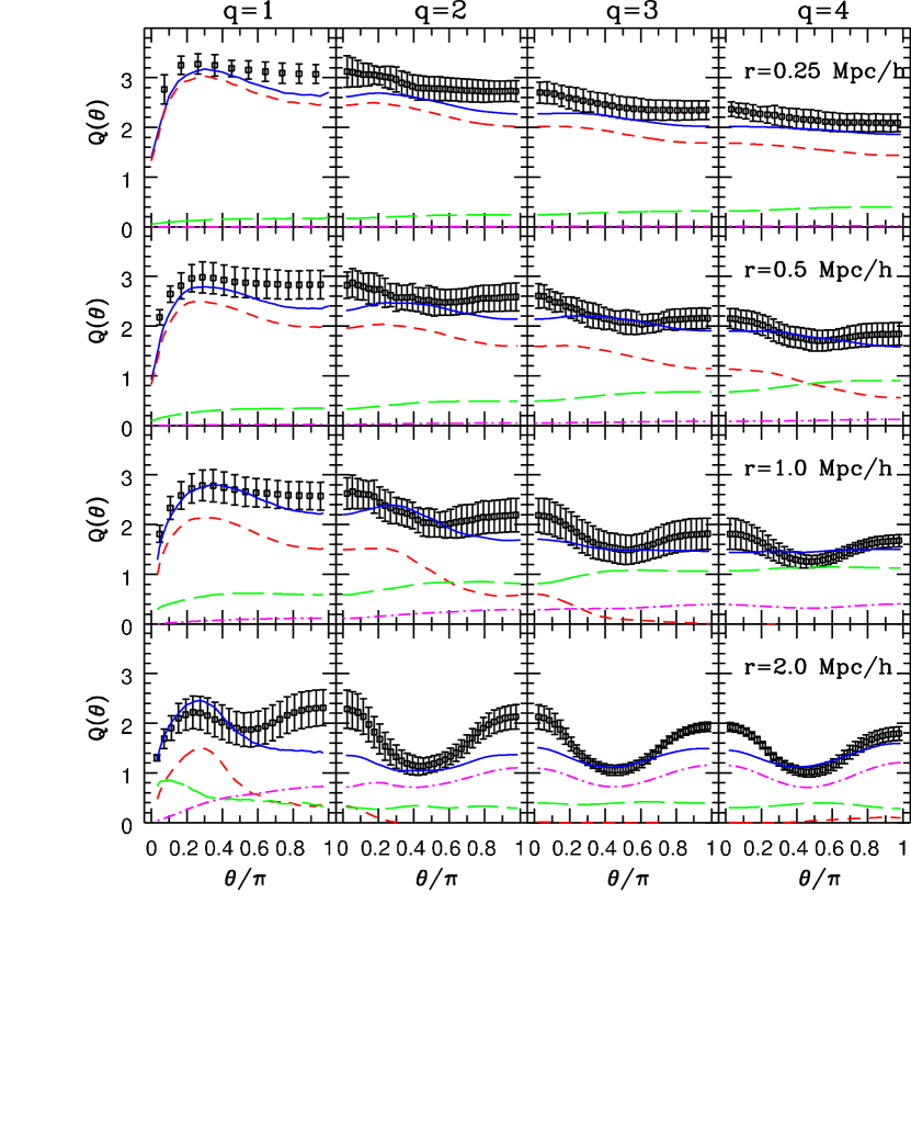
Figure 10: Same as Fig.9 but for the reduced 3PCF. Halo model reproduces simulations reasonably well, specially for intermediate angles, what is in agreement with Fig.8 that shows equilateral triangles alone. The discrepancy with simulations becomes more evident in this ratio statistic, as it combines the complicated configuration dependences of both 2PCF and 3PCF. As in Fig.9, the discrepancy becomes more significant for $\rm{r}\lower 2.15277pt\hbox{$\;\buildrel>\over{\sim}\;$}0.5~{}\rm{Mpc/h}$.

Fig.10 shows the reduced 3PCF $Q(r)$ for the same triangles whereas Fig.11 shows an interpolated surface displaying the $(\theta,q)$ dependence for the mean values of the N-body for $\rm{r}=2~{}\rm{Mpc/h}$. Note that since $Q(r)$ is predicted to be of order unity for all configurations, it is more suitable for high-precision comparisons on linear scale plots. On the down side, the complex structure of this ratio statistic combining 2PCF and 3PCF complicates interpretation. In particular, halo model describes the configuration dependence of the reduced 3PCF accurately for $\rm{r}\lower 2.15277pt\hbox{$\;\buildrel<\over{\sim}\;$}0.5\rm{Mpc/h}$, but it becomes increasingly inaccurate for larger scales. The slight overall amplitude mismatch observed (see e.g., the case for isosceles triangles, $q=1$, in left column of Fig.10) is due to the halo model 2PCF overpredicting simulations. We have checked that using fitting formula of (Smith et al., 2003) for the 2PCF instead of the halo model does not improve the agreement with simulations significantly. Note that for intermediate angles theoretical predictions always agree with the simulations, in line with our earlier results for equilateral triangles (see Fig.8). The most visible difference between model and N-body results is the lack of configuration dependence predicted by the halo model on larger scales, $\rm{r}~{}\lower 2.15277pt\hbox{$\;\buildrel>\over{\sim}\;$}0.5\rm{Mpc/h}$.

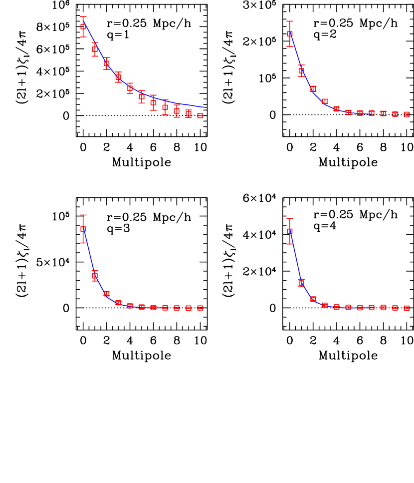
Figure 12: Harmonic multipoles of the 3PCF at $\rm{r}=0.25~{}\rm{Mpc/h}$: theoretical predictions are in excellent agreement with simulations. Only lower order multipoles ($\ell\lower 2.15277pt\hbox{$\;\buildrel<\over{\sim}\;$}5$, except for isosceles triangles) have a non-zero contribution.

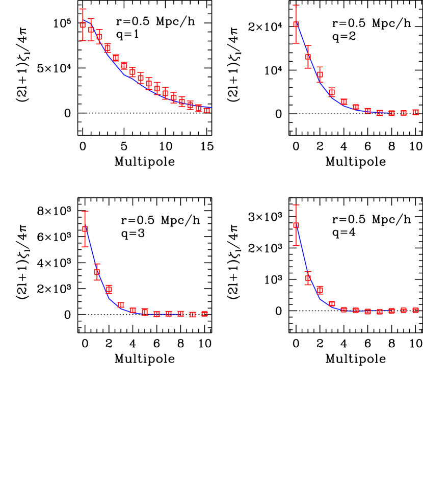
Figure 13: Same as Fig.12 but for $\rm{r}=0.5~{}\rm{Mpc/h}$.

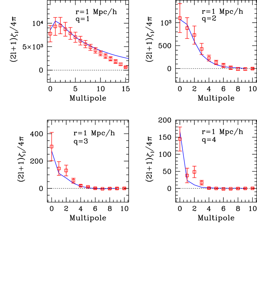
Figure 14: Same as Fig.12 but for $\rm{r}=1~{}\rm{Mpc/h}$. Note how the higher multipoles becomes significant for isosceles triangles ($q=1$), and that theoretical predictions tend to underestimate the quadrupole moment for $q>1$.

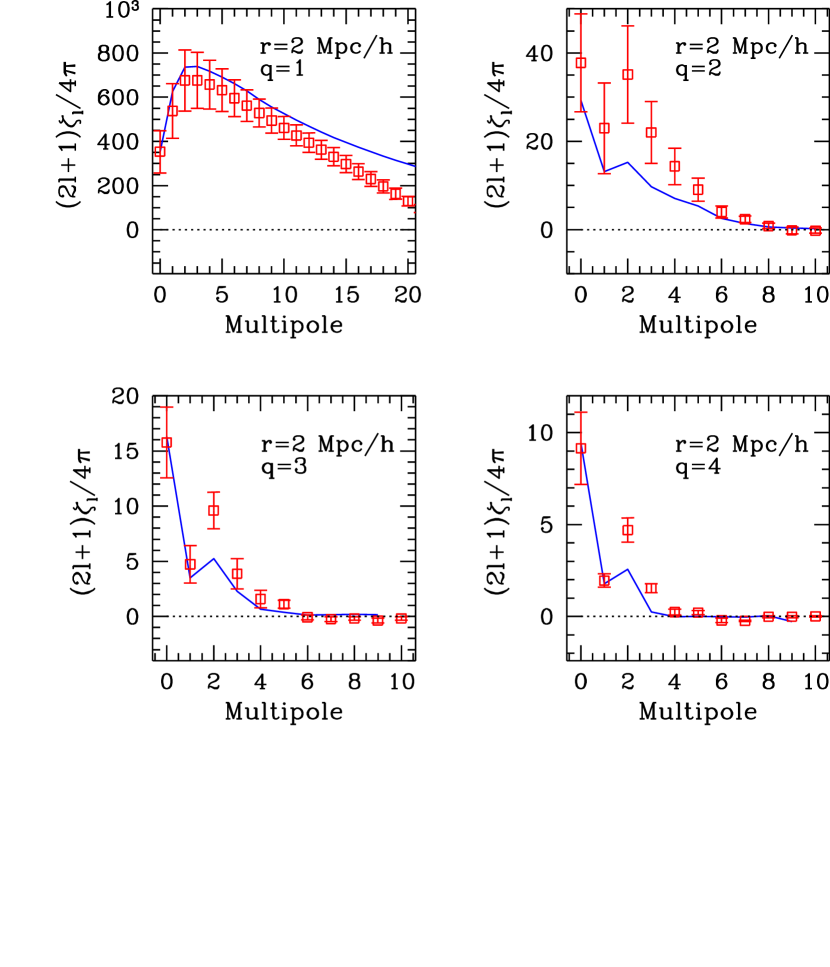
Figure 15: Same as Fig.12 but for $\rm{r}=2~{}\rm{Mpc/h}$. In line with Fig.14, it shows that halo model clearly underpredicts the quadrupole (and to a lesser extent, the octopole) observed in numerical simulations. This quadrupole deficit explains the lack of $\theta$-dependence in halo model predictions for $Q(r,q,\theta)$, as shown in the lower rows of Fig.10.

The multipole expansion of the 3PCF, eq.(12), is particularly useful to pinpoint why the halo model fails to reproduce numerical results. Figs.12-15 show the 3PCF multipoles for different triangles and scales $\rm{r}=0.25-2~{}\rm{Mpc/h}$. In general, the amplitude of the coefficients falls off rapidly with multipole order. This makes multipoles especially convenient to compress information in the cosmological 3PCF in the non-linear regime (see also Szapudi, 2004).

Isosceles triangles are exceptional: on small angles the third side of the triangle is very small, which results in a rapid increase. This can be described in multipole space only with a high number of multipoles (such as a Dirac $\delta$-function would have infinite number of multipoles). The situation worsens towards larger scales, due to even more rapid increase of the 3PCF on small angles. While this technical deficiency can be overcome by simply smoothing the correlation function over angles (“band limiting”), we note that on scales above $\rm{r}~{}\lower 2.15277pt\hbox{$\;\buildrel>\over{\sim}\;$}5\rm{Mpc/h}$, where this effect becomes severe, PT becomes more and more accurate, therefore halo models are not necessary for dark matter predictions (Fry, 1984; Jing & Boerner, 1997; Barriga & Gaztañaga, 2002).

More interestingly, for $\rm{r}~{}\lower 2.15277pt\hbox{$\;\buildrel>\over{\sim}\;$}0.5\rm{Mpc/h}$, halo model consistently underpredicts the quadrupole moment (and to a lesser extent, the octopole). The observed lack of configuration dependence in the halo model with respect to simulations is primarily due to a quadrupole deficit in the prediction (see Figs.9 and 10). This might be caused by the 2-halo term, which shows hardly any variation with angle on large-scales $\rm{r}~{}\lower 2.15277pt\hbox{$\;\buildrel>\over{\sim}\;$}0.5\rm{Mpc/h}$ (see Figs.9 and 10), contrary to what one would expect for halo-halo spatial correlations. One possible reason for this quadrupole deficit in the two-halo term is that our implementation of the halo model assumes that haloes are spherical, whereas real virialized objects in high-resolution CDM simulations do have a typically asymmetric (triaxial) shape (see e.g.,  Barnes & Efstathiou, 1987; Jing & Suto, 2002; Moore et al., 2004). SSHJ already pointed out in their bispectrum analysis that relaxing the sphericity hypothesis for halo shapes could bring halo model to a closer agreement with the configuration dependence observed in numerical simulations. Although our analysis suggests a similar conclusion, it is unclear whether one-halo (as pointed out by SSHJ) or rather two-halo terms (that show a significant lack of configuration dependence at all scales) should carry the missing quadrupole.

On the other hand halo substructure (Sheth, 2003; Sheth & Jain, 2003) could play a significant role on scales comparable to large-cluster sized haloes  $1\rm{Mpc/h}$. However, a recent analysis (Dolney et al., 2004) suggests that substructure tends to attenuate the amplitude of the reduced bispectrum on small scales. This would render our analytic predictions, at least our fiducial model, in disagreement with N-body measurements (see Figs. 5 and 6).

Clearly, there are other potential improvements to our implementation of the halo model, most importantly a consistent definition of the mass function for a modified halo boundary (see White, 2002; Hu & Kravtsov, 2003), or allowing for a steeper inner halo profile (see Moore et al., 1998) what could bring model predictions closer to measurements in high-resolution N-body simulations. We plan to address these issues in future work.

5 Conclusions

The revival of the halo model in recent years has been triggered by the ability of high-resolution N-body simulations to test theoretical predictions with great precision. In this paper we have presented a detailed comparison of halo model predictions against simulations for the 2PCF and 3PCF in real and Fourier space. Our analysis has focused on the transition scales, $\rm{r}\approx 0.25-5\rm{Mpc/h}$ that connect large (quasi-linear) scales, appropriately described by PT, with highly non-linear scales where phenomena such as the stable clustering hypothesis require higher resolution simulations to be accurately tested.

Our results show that halo boundary and mass function cut-off have a significant effect on the three-point correlation functions on these transition scales, and thus these statistics can be used to constrain such halo model parameters. A fiducial model with halo boundary $\rm{r}=1.3{R_{v}}~{}\rm{Mpc/h}$ and mass cut-off $M_{cut}=10^{15}~{}\rm{M}_{\sun}$ brings theoretical predictions in close agreement to our simulations. The success of our fiducial model in explaining non-linear gravitational clustering has been comprehensively demonstrated in Fourier space for the power spectrum (Fig.4), the reduced bispectrum (Figs.5 and 6), as well as in real space, through the two-point correlation function (Figs.2 and 3), 3PCF (Fig.9), and the reduced 3PCF (Figs.8, and 10) along with its multipole moments (Figs.12-15).

Halo model predictions are in good agreement with the configuration and scale dependence of the reduced bispectrum at all the scales measured in N-body results, $k=0.25-1~{}\rm{h/Mpc}$. On the other hand, while the model correctly predicts the amplitudes of the 3PCF on intermediate angles for all the scales tested, it exhibits a lack of configuration dependence that becomes more significant on scales larger than the largest halos seen in simulations $\rm{r}\lower 2.15277pt\hbox{$\;\buildrel>\over{\sim}\;$}1~{}\rm{Mpc/h}$. Although the reason for this is not clear, we suggest that non-spherical haloes could produce a more pronounced configuration dependence in theoretical predictions. This could be realized through the two-halo terms that show a rather flat behavior in the current implementation of the model. However if the orientation of the two halos is random, the non-sphericity should cancel out. This issue certainly deserves further attention in future analyses of the dark-matter and galaxy N-point correlation functions.

It is particularly useful to decompose the reduced 3PCF in its harmonic multipoles $Q_{\ell}$’s, as given by eq(17). We have seen that only the lowest orders have non-zero amplitude and thus the non-linear 3PCF can be compressed in a few numbers (see Fig. 1). Furthermore, assuming a model for the halo occupation distribution and an appropriate modeling of redshift distortions, one should be able to formally decompose the 3PCF of galaxies in the exact same way. In particular, observables such as the harmonic multipoles of the galaxy 3PCF measured in large volume surveys should be largely uncorrelated and approximately Gaussian distributed, in a similar way it happens for the angular power spectrum multipoles of the CMB anisotropy $C_{\ell}$.

Thus the $Q_{\ell}$’s must be tightly related to the signal-to-noise eigenmodes of the 3PCF (Scoccimarro, 2000; Gaztanaga & Scoccimarro, 2005). Moreover Gaztanaga & Scoccimarro (2005) have shown that the highest signal-to-noise Q-eigenmodes measured in mock galaxy catalogs can be efficiently used to recover bias parameters. It is remarkable that the first three Q-eigenmodes have a configuration dependence that is extremely similar to the monopole, dipole and quadrupole terms (compare their Fig.10 with middle panels in Fig.1 of this paper). This suggests that the $Q_{\ell}$’s are indeed closely related to the uncorrelated modes of the galaxy 3PCF and thus they may simplify the procedure of constraining galaxy bias from the 3PCF.

Alternatively, the proposed multipole approach can be readily applied to other clustering statistics of the mass density field in the non-linear regime such as the projected mass 3PCF, that is barely affected by redshift distortions (see Zheng, 2004, for a recent implementation using Fourier series), or the 3PCF of the convergence field that probes the lensing potential (see e.g.,  Takada & Jain, 2003b).

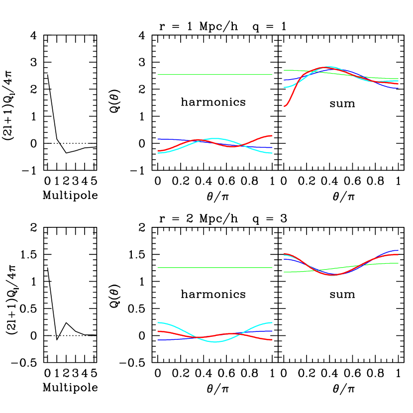
Figure 1: Reconstructing the 3PCF form its harmonics. Only the lowest harmonic coefficients are non-zero (see left panels). Middle panels show the configuration dependence of individual harmonic terms i.e. harmonic coefficients times the Legendre polynomials. We display terms $\ell=0,1,2$ and $3$ using increasingly thicker lines. Right panels show the sum over harmonics up to a given $\ell_{max}=1,2,3$ and $10$ (from thin to thick lines). In general, the non-linear 3PCF is dominated by the monopole, that sets the amplitude, and quadrupole, that shapes the configuration dependence. Top panels show isosceles triangles of length $r=1~{}\rm{Mpc/h}$, while lower panels display more elongated triangles with basic length $r=2~{}\rm{Mpc/h}$ and length-ratio $q=3$.

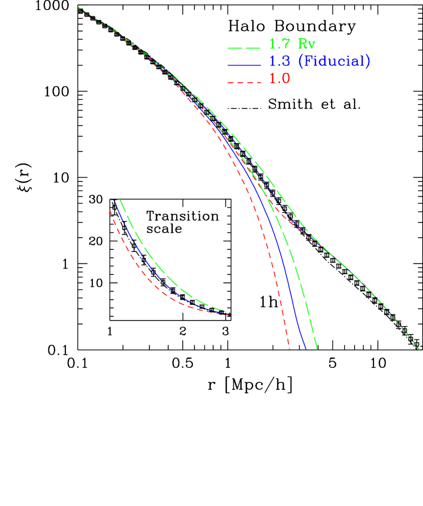
Figure 2: Halo boundary effects on the 2PCF: defining halo boundary at $\rm{r}={R_{v}}$ underestimates $\xi(r)$ on the transition scales. Larger boundaries yield a larger one-halo (1h) contribution. For $\rm{r}=1.3~{}{R_{v}}$ (solid line), we find good agreement with N-body results. The inset shows a blow-up of the transitions scales, where our fiducial model agrees well with numerical results and the Smith et al. (2003) fitting function. On larger scales the fiducial model overpredicts numerical simulations, but converges to them for $\rm{r}\lower 2.15277pt\hbox{$\;\buildrel>\over{\sim}\;$}20\rm{Mpc/h}$.

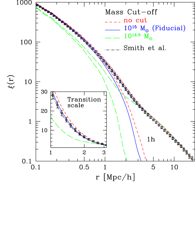
Figure 3: Same as Fig.2 for the mass cut-off: in order to mimic the absence of haloes of mass $M>M_{cut}$ in simulations, our fiducial model incorporates a cut-off in the mass function, $M_{cut}=10^{15}\rm{M}_{\sun}$ (solid line), what lowers the 2PCF on non-linear scales (i.e. those dominated by the one-halo term). The Smith et al. fitting function is only shown in the inset for clarity.

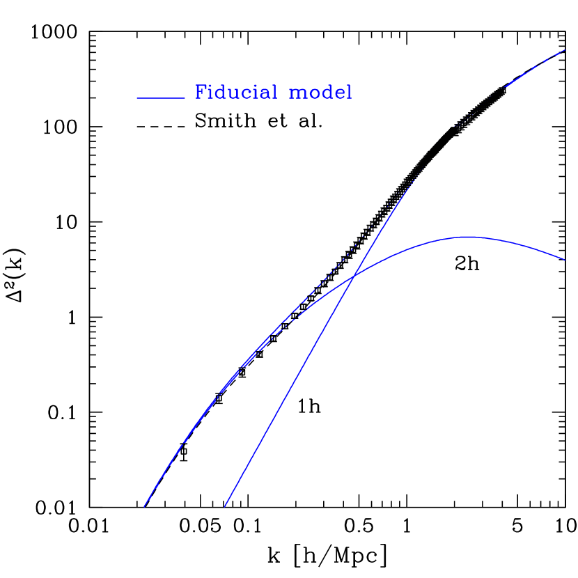
Figure 4: Mass power-spectrum per logarithmic wavenumber, $\Delta^{2}(k)=k^{3}P(k)/2\pi^{2}$, in the fiducial halo model (solid line, see text for details) compared to N-body simulations (symbols). One (1h) and two (2h) halo contributions are shown to have comparable amplitude in the transition scales $k\approx 0.5~{}\rm{h/Mpc}$. For reference, it is also shown a fitting function to numerical simulations (dashed line; Smith et al. (2003)). Halo model agrees very well with N-body except on scales $k\approx 0.1-0.5~{}\rm{h/Mpc}$, where it tends to slightly overpredict numerical simulations. Note that we use a box-size $L=239.5~{}\rm{Mpc/h}$ for small scales, $k\lower 2.15277pt\hbox{$\;\buildrel>\over{\sim}\;$}2~{}\rm{h/Mpc}$, whereas a larger box (VLS) simulation $L=479~{}\rm{Mpc/h}$ is used for larger scales, $k\lower 2.15277pt\hbox{$\;\buildrel<\over{\sim}\;$}2~{}\rm{h/Mpc}$.

Figure 11: Smoothly interpolated surface showing the configuration dependence of the reduced 3PCF at $\rm{r}=2~{}\rm{Mpc/h}$ from N-body simulations. It exhibits a symmetric convex shape, what is in qualitative agreement with predictions from the three-halo term in the halo model. For isosceles triangles this symmetry is broken at small-angles due to non-linear effects, as reproduced by the one-halo contribution (see Fig.10).

We would like to thank J.Fry, E.Gaztañaga, R.Scoccimarro and M.Takada for useful comments and discussions. PF ackowledges support from the spanish MEC through a Ramón y Cajal fellowship and project AYA2002-00850 with EU-FEDER funding. This research was supported by NASA through ATP NASA NAG5-12101 and AISR NAG5-11996, as well as by NSF grants AST02-06243 and ITR 1120201-128440. JP acknowledges support by PPARC through PPA/G/S/2000/00057.

References

- Barnes & Efstathiou (1987) Barnes, J., & Efstathiou, G. 1987, ApJ, 319, 575
- Barriga & Gaztañaga (2002) Barriga, J., & Gaztañaga, E. 2002, MNRAS, 333, 443
- Berlind & Weinberg (2002) Berlind, A. A., & Weinberg, D. H. 2002, ApJ, 575, 587
- Berlind et al. (2003) Berlind, A. A., et al. 2003, ApJ, 593, 1
- Bond & Efstathiou (1984) Bond, J. R., & Efstathiou, G. 1984, ApJ, 285, L45
- Bullock et al. (2001) Bullock, J. S., Kolatt, T. S., Sigad, Y., Somerville, R. S., Kravtsov, A. V., Klypin, A. A., Primack, J. R., & Dekel, A. 2001, MNRAS, 321, 559
- Cooray & Hu (2001) Cooray, A., & Hu, W. 2001, ApJ, 548, 7
- Cooray & Sheth (2002) Cooray, A., & Sheth, R. 2002, Phys. Rep., 372, 1
- Couchman et al. (1995) Couchman, H. M. P., Thomas, P. A., & Pearce, F. R. 1995, ApJ, 452, 797
- Dolney et al. (2004) Dolney, D., Jain, B., & Takada, M. 2004, MNRAS, 352, 1019
- Fry (1984) Fry, J. N. 1984, ApJ, 279, 499
- Gaztanaga & Scoccimarro (2005) Gaztanaga, E., & Scoccimarro, R. 2005, ArXiv Astrophysics e-prints
- Gray et al. (2004) Gray, A. G., Moore, A. W., Nichol, R. C., Connolly, A. J., Genovese, C., & Wasserman, L. 2004, in Astronomical Society of the Pacific Conference Series, 249
- Hu & Kravtsov (2003) Hu, W., & Kravtsov, A. V. 2003, ApJ, 584, 702
- Jenkins et al. (2001) Jenkins, A., Frenk, C. S., White, S. D. M., Colberg, J. M., Cole, S., Evrard, A. E., Couchman, H. M. P., & Yoshida, N. 2001, MNRAS, 321, 372
- Jing & Boerner (1997) Jing, Y. P., & Boerner, G. 1997, A&A, 318, 667
- Jing & Suto (2002) Jing, Y. P., & Suto, Y. 2002, ApJ, 574, 538
- Ma & Fry (2000a) Ma, C., & Fry, J. N. 2000a, ApJ, 543, 503
- Ma & Fry (2000b) Ma, C., & Fry, J. N. 2000b, ApJ, 531, L87
- Macfarland et al. (1998) Macfarland, T., Couchman, H. M. P., Pearce, F. R., & Pichlmeier, J. 1998, New Astronomy, 3, 687
- McClelland & Silk (1977a) McClelland, J., & Silk, J. 1977a, ApJ, 216, 665
- McClelland & Silk (1977b) McClelland, J., & Silk, J. 1977b, ApJ, 217, 331
- McClelland & Silk (1978) McClelland, J., & Silk, J. 1978, ApJS, 36, 389
- Mo & White (1996) Mo, H. J., & White, S. D. M. 1996, MNRAS, 282, 347
- Moore et al. (2001) Moore, A. W., Connolly, A. J., Genovese, C., Gray, A., Grone, L., & et al.. 2001, in Mining the Sky, 71
- Moore et al. (1998) Moore, B., Governato, F., Quinn, T., Stadel, J., & Lake, G. 1998, ApJ, 499, L5
- Moore et al. (2004) Moore, B., Kazantzidis, S., Diemand, J., & Stadel, J. 2004, MNRAS, 354, 522
- Navarro et al. (1997) Navarro, J. F., Frenk, C. S., & White, S. D. M. 1997, ApJ, 490, 493
- Neyman & Scott (1952) Neyman, J., & Scott, E. L. 1952, ApJ, 116, 144
- Peacock & Smith (2000) Peacock, J. A., & Smith, R. E. 2000, MNRAS, 318, 1144
- Peebles (1974) Peebles, P. J. E. 1974, A&A, 32, 197
- Scherrer & Bertschinger (1991) Scherrer, R. J., & Bertschinger, E. 1991, ApJ, 381, 349
- Scoccimarro (2000) Scoccimarro, R. 2000, ApJ, 544, 597
- Scoccimarro et al. (1998) Scoccimarro, R., Colombi, S., Fry, J. N., Frieman, J. A., Hivon, E., & Melott, A. 1998, ApJ, 496, 586
- Scoccimarro et al. (2001) Scoccimarro, R., Sheth, R. K., Hui, L., & Jain, B. 2001, ApJ, 546, 20
- Seljak (2000) Seljak, U. 2000, MNRAS, 318, 203
- Sheth (2003) Sheth, R. K. 2003, MNRAS, 345, 1200
- Sheth & Jain (1997) Sheth, R. K., & Jain, B. 1997, MNRAS, 285, 231
- Sheth & Jain (2003) Sheth, R. K., & Jain, B. 2003, MNRAS, 345, 529
- Sheth & Tormen (1999) Sheth, R. K., & Tormen, G. 1999, MNRAS, 308, 119
- Smith et al. (2003) Smith, R. E., et al. 2003, MNRAS, 341, 1311
- Szapudi (2004) Szapudi, I. 2004, ApJ, 605, L89
- Szapudi & Szalay (1998) Szapudi, S., & Szalay, A. S. 1998, ApJ, 494, L41
- Takada & Jain (2003a) Takada, M., & Jain, B. 2003a, MNRAS, 340, 580
- Takada & Jain (2003b) Takada, M., & Jain, B. 2003b, MNRAS, 344, 857
- Wang et al. (2004) Wang, Y., Yang, X., Mo, H. J., van den Bosch, F. C., & Chu, Y. 2004, MNRAS, 353, 287
- White (2002) White, M. 2002, ApJS, 143, 241
- Zehavi et al. (2004) Zehavi, I., et al. 2004, ApJ, 608, 16
- Zheng (2004) Zheng, Z. 2004, ApJ, 614, 527