Metal abundances in extremely distant Galactic old open clusters.
II. Berkeley 22 and Berkeley 66¹

Abstract

We report on high resolution spectroscopy of four giant stars in the Galactic old open clusters Berkeley 22 and Berkeley 66 obtained with HIRES at the Keck telescope. We find that $[Fe/H]=-0.32\pm 0.19$ and $[Fe/H]=-0.48\pm 0.24$ for Berkeley 22 and Berkeley 66, respectively. Based on these data, we first revise the fundamental parameters of the clusters, and then discuss them in the context of the Galactic disk radial abundance gradient. We found that both clusters nicely obey the most updated estimate of the slope of the gradient from Friel et al. (2002) and are genuine Galactic disk objects.

1 Introduction

This paper is the second of a series dedicated at obtaining high resolution spectroscopy of distant Galactic old open cluster giant stars to derive new or improved estimates of their metal content. In Carraro et al. (2004) we presented results for Berkeley 29 and Saurer 1, the two old open clusters possessing the largest galactocentric distance known, and showed that they do not belong to the disk, but to the Monoceros feature (see also the discussion in Frinchaboy et al. 2005). Here we present high-resolution spectra of four giant stars in the old open clusters Berkeley 22 and Berkeley 66. The latter cluster, in particular, is of particular interest, since its heliocentric distance is among the largest currently known.
With this paper we aim to enlarge the sample of old open clusters with metallicity obtained from high resolution spectra, and to test the common assumption of axisymmetry made in chemical evolution models about the structure of the Milky Way disk. For this purpose we selected two open clusters with about the same age located one (Berkeley 66) in the second Galactic Quadrant, and the other (Berkeley 22) in the third Galactic Quadrant. Significant differences in metal abundance for clusters located in different disk zones would hopefully provide useful clues about the chemical evolution of the disk and about the role of accretion and infall phenomena.
The layout of the paper is as follows. Sections 2 and 3 illustrate the observations and the data reduction strategies, while Section 4 deals with radial velocity determinations. In Section 5 we derive the stellar abundances and in Section 6 we revise the cluster fundamental parameters. The radial abundance gradient and the abundance ratios are discussed in Section 7 and 8, respectively. The results of this paper are finally discussed in Section 9

2 Observations

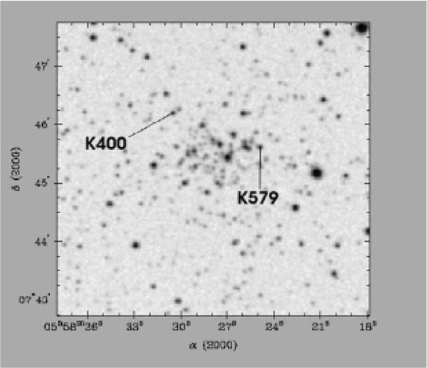
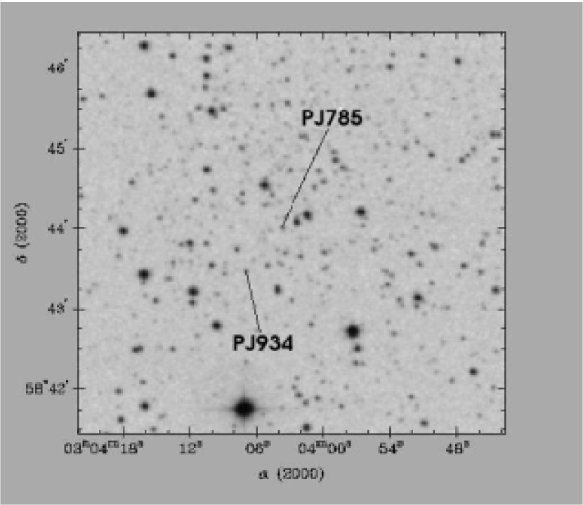
Figure 1: Digital Sky Survey finding charts of the observed stars in Berkeley 22 (left panel) and Berkeley 66 (right panel)

The observations were carried out on the night of November 30, 2004 at the W.M. Keck Observatory under photometric conditions and typical seeing of 1$\farcs$1 arcsec. The HIRES spectrograph (Vogt et al., 1994) on the Keck I telescope was used with a 1$\farcs$1 x 7″ slit to provide a spectral resolution R = 34,000 in the wavelength range 5200$-$8900 Å on the three 2048$\times$4096 CCDs of the mosaic detector. A blocking filter was used to remove second-order contamination from blue wavelengths. Three exposures of 1500–1800 seconds were obtained for the stars Berkeley 22$-$400 and Berkeley 22$-$579. For both Berkeley 66$-$785 and Berkeley 66$-$934 we took four exposures of 2700 seconds each. During the first part of the night, when the telescope pointed to Berkeley 66, the observing conditions were far from optimal, due to the presence of thick clouds. For this reason our abundance analysis in this first cluster is limited to Berkeley 66$-$785. For the wavelength calibration, spectra of a thorium-argon lamp were secured after the set of exposures for each star was completed. The radial velocity standard HD 82106 was observed at the end of the night.
In Fig. 1 we show a finding chart for the two clusters where the four observed stars are indicated, while in Fig. 2 we show the position of the stars in the Color$-$Magnitude Diagram (CMD), based on published photometry (Kaluzny 1994, Phelps & Janes 1996).

3 Data Reduction

Images were reduced using IRAF, including bias subtraction, flat-field correction, frame combination, extraction of spectral orders, wavelength calibration, sky subtraction and spectral rectification. The single orders were merged into a single spectrum. As an example, we show in Fig. 3 a portion of the reduced, normalized spectrum of Be 22-400.

4 Radial Velocities

No radial velocity estimates were previously available for Berkeley 22 and Berkeley 66. The radial velocities of the target stars were measured using the IRAF FXCOR task, which cross-correlates the object spectrum with the template (HD 82106). The peak of the cross-correlation was fitted with a Gaussian curve after rejecting the spectral regions contaminated by telluric lines ($\lambda>6850$ Å). In order to check our wavelength calibration we also measured the radial velocity of HD 82106 itself, by cross-correlation with a solar-spectrum template. We obtained a radial heliocentric velocity of 29.8$\pm$0.1 km s^-1, which perfectly matches the published value (29.7 km/sec; Udry et al. 1999). The final error in the radial velocities was typically about 0.2 km s^-1. The two stars we measured in each clusters have compatible radial velocities (see Table 1), and are considered, therefore, bona fide cluster members.

5 ABUNDANCE ANALYSIS

5.1 Atomic parameters and equivalent widths

We derived equivalent widths of spectral lines by using the standard IRAF routine SPLOT. Repeated measurements show a typical error of about 5$-$10 mÅ, also for the weakest lines. The line list (FeI, FeII, Mg, Si, Ca, Al,, Na, Ni and Ti, see Table 3) was taken from Friel et al. (2003), who considered only lines with equivalent widths narrower than 150mÅ, in order to avoid non-linear effects in the LTE analysis of the spectral features. log(gf) parameters of these lines were re-determinated using equivalent widths from the solar-spectrum template, solar abundances from Anders & Grevesse (1989) and standard solar parameters ($T_{eff}=5777~{}K,log(g)=4.44,v_{t}=0.8~{}Km\,s^{-1}$).

5.2 Atmospheric parameters

Initial estimates of the atmospheric parameter $T_{eff}$ were obtained from photometric observations in the optical. BVI data were available for Berkeley 22 (Kaluzny, 1994), while VI photometry for Berkeley 66 has been taken from (Phelps & Janes, 1996). Reddening values are E(B$-$V)= 0.62 (E(V$-$I)= 0.74), and E(V$-$I)= 1.60, respectively. First guess effective temperatures were derived from the (V$-$I)–$T_{eff}$ and (B$-$V)–$T_{eff}$ relations, the former from Alonso et al. (1999) and the latter from Gratton et al. (1996). We then adjusted the effective temperature by minimizing the slope of the abundances obtained from Fe I lines with respect to the excitation potential in the curve of growth analysis. For both clusters the derived temperature yields a reddening consistent with the photometric one.
Initial guesses for the gravity $\log$(g) were derived from:

$$log(\frac{g}{g_{\odot}})=log(\frac{M}{M_{\odot}})+4\times log(\frac{T_{eff}}{T_{\odot}})-log(\frac{L}{L_{\odot}})$$ (1)

taken from Carretta & Gratton (1997). In this equation the mass $\frac{M}{M_{\odot}}$ was derived from the comparison between the position of the star in the Hertzsprung$-$Russell diagram and the Padova Isochrones (Girardi et al., 2000). The luminosity $\frac{L}{L_{\odot}}$ was derived from the the absolute magnitude $M_{V}$, assuming the literature distance moduli of 15.9 for Berkeley 22 (Kaluzny, 1994) and 17.4 for Berkeley 66 (Phelps & Janes, 1996). The bolometric correction (BC) was derived from the relation BC–$T_{eff}$ from Alonso et al. (1999). The input $\log$(g) values were then adjusted in order to satisfy the ionization equilibrium of Fe I and Fe II during the abundance analysis. Finally, the micro$-$turbulence velocity is given by the following relation (Gratton et al., 1996):

$$v_{t}[km\,s^{-1}]=1.19\times 10^{-3}\times T_{eff}-0.90\times log(g)-2$$ (2)

The final adopted parameters are listed in Table 2.

5.3 Abundance determination

The LTE abundance program MOOG (freely distributed by Chris Sneden, University of Texas, Austin) was used to determine the metal abundances. Model atmospheres were interpolated from the grid of Kurucz (1992) models by using the values of $T_{eff}$ and $\log$(g) determined as explained in the previous section. During the abundance analysis $T_{eff}$, $\log$(g) and $v_{t}$ were adjusted to remove trends in excitation potential, ionization equilibrium and equivalent width for Fe I and Fe II lines. Table 3 contains the atomic parameters and equivalent widths for the lines used. The first column contains the name of the element, the second the wavelength in Å, the third the excitation potential, the fourth the oscillator strength $\log$ (gf), and the remaining ones the equivalent widths of the lines for the observed stars.
The derived abundances are listed in Table 4, together with their uncertainties. The measured iron abundances are [Fe/H]=$-$0.32$\pm 0.19$ and [Fe/H]=$-$0.48$\pm 0.24$ for Berkeley 22 and Berkeley 66, respectively. The reported errors are derived from the uncertainties on the single star abundance determination (see Table 4). For Berkeley 66$-$934 no abundance determination was possible because the S/N ratio in our spectrum was too low to perform any equivalent width determination.

Finally, using the stellar parameters (colors, T_eff and log(g)) and the absolute calibration of the MK system (Straizys et al. 1981), we derived the stellar spectral classification, which we provide in Table 1.

6 REVISION OF CLUSTER PROPERTIES

Our study is the first to provide spectral abundance determinations of stars in Berkeley 22 and Berkeley 66. Here we briefly discuss the revision of the properties of these two clusters which follow from our measured chemical abundances (see Figs. 4 and 5). We use the isochrone fitting method and adopt for this purpose the Padova models from Girardi et al. (2000).

6.1 Berkeley 22

Berkeley 22 is an old open cluster located in the third Galactic quadrant, first studied by Kaluzny (1994). On the basis of deep VI photometry he derived an age of 3 Gyr, a distance of 6.0 Kpc and a reddening E(V$-$I)=0.74. The author suggests that the probable metal content of the cluster is lower than solar. Here we obtained [Fe/H]=$-$0.32, which corresponds to Z=0.008 and roughly half the solar metal content. Very recently Di Fabrizio et al. (2005) presented new BVI photometry, on the basis of which they derive a younger age (2.0-2.5 Gyr), but similar reddening and distance, also suggesting that the cluster posseses solar metal abundance. The two photometric studies are compatible in the VI filters, being the difference in the V and I zeropoints less than 0.03 mag. Both the studies show that the cluster turnoff is located at V = 19 and a clump at V = 16.65.
According to Carraro & Chiosi (1994), with a $\Delta V\approx 2.35$ mag ($\Delta V$ being the magnitude difference between the turnoff and the clump) and for the derived metallicity, one would expect an age around 3.5 Gyr. This preliminary estimate of the age is in fact confirmed by the isochrone fitting method. In Fig. 4 the solid line is a 3.3 Gyr isochrone, which provides a new age estimate of 3.3$\pm$0.3 Gyrs for the same photometric reddening and Galactocentric distance derived by Kaluzny (1994). Both the turnoff and the clump location are nicely reproduced. The uncertainty reflects the range of isochrones which produce an acceptable fit.
For comparison, in the same figure we over-impose a solar metallicity isochrone for the age of 2.25 Gyr (dashed line in Fig. 4), and for the same reddening and distance reported by Di Fabrizio et al. (2005). This isochrone clearly does not provide a comparable good fit. When trying to fit the turnoff, both the color of the Red Giant Branch and the position of the clump cannot be reproduced.

6.2 Berkeley 66

Berkeley 66 was studied by Guarnieri & Carraro (1997) and Phelps & Janes (1996), who suggested a reddening E(V$-$I)=1.60 and a metallicity in the range $-0.23\leq[Fe/H]\leq 0.0$. By assuming these values, Phelps & Janes (1996) derived a galactocentric distance of 12.9 Kpc and an age of 3.5 Gyrs. We obtain a significantly smaller abundance value [Fe/H]=$-$0.48$\pm$0.24 for a spectroscopic reddening of E(V$-$I)=1.60, which is consistent with the Phelps & Janes (1996) estimate. By looking at the CMD, the turnoff is situated at V = 20.75, whereas the clump is at V = 18.25, implying a $\Delta V$ of 2.5. For this $\Delta V$ and the derived [Fe/H], the Carraro & Chiosi (1994) calibration yields an age of about 4.7 Gry, significantly larger than previous estimate. The value [Fe/H]=$-$0.48 tanslates into Z=0.006, and we generated a few isochrones for this exact metal abundance from Girardi et al. (2000). The result is shown in Fig 5, where a 4 and 5 Gyr isochrones (dashed and solid line, respectively) are overimposed to the cluster CMD. Both the isochrones reasonably reproduce the turnoff shape but the 5 Gyr one (solid line) clearly presents a too bright clump. On the other hand, the 4 Gyr isochrone reproduces well all the CMD feature. This new age estimate provides a reddening E(V-I) = 1.60 and a heliocentric distance of 5 Kpc.

7 THE RADIAL ABUNDANCE GRADIENT

In Fig. 6 we plot the open cluster Galactic radial abundance gradient, as derived from Friel et al. (2002), which is at present the most updated version of the gradient itself. The clusters included in their work (open squares) define an overall slope of $-$0.06$\pm$0.01 dex Kpc^-1 (solid line). The filled circles represent the two clusters analyzed here, and it can be seen that they clearly follow very nicely the general trend. In fact the dashed line, which represents the radial abundance gradient determined by including Berkeley 22 and Berkeley 66, basically coincides with the Friel et al. (2002) one.
We note that the gradient exhibits quite a significant scatter. One may wonder whether this solely depends on observational errors, or whether this scatter reflects a true chemical inhomogeneity in the Galactic disk.
It must be noted however that between 10 and 14 kpc the scatter increases and the distribution of the cluster abundances is compatible also with a flat gradient. Again, it is extremely difficult to conclude whether this behaviour of the gradient is significant, or whether the distribution of abundances is mostly affected by the size of the observational errors and the small number of clusters involved.

8 ABUNDANCE RATIOS

Abundance ratios constitute a powerfull tool to assign a cluster to a stellar population Friel et al. 2003. In PaperI (Carraro et al. 2004) we found that Saurer 1 and Berkeley 29 exhibit enhanced abundance ratio with respect to the Sun, and we concluded that they probably do not belong to the Galactic disk, since all the old open cluster for which detailed abundance analysis is available show solar scaled abundance ratios.
In Table 5 we list the abundance ratios for the observed stars in Berkeley 22 and Berkeley 66. Our program clusters have ages around 3-4 Gyrs and iron metal content [Fe/H] $\approx$ $-$0.3-0.4. They are therefore easily comparable with similar clusters from the literature, such as Tombaugh 2 and Melotte 66 (see Friel et al. 2003, Tab. 7). We note that the latter two clusters and our program clusters have scaled solar abundances. Indeed, at a similar [Fe/H] and age , Berkeley 22 and Melotte 66 have similar values for all the abundance ratios.
Similar conclusions can be drawn for Berkeley 66, when compared with Tombaugh 2, an old open cluster of similar age and [Fe/H]. All the abundance ratios we could measure are comparable in these two clusters.
These results therefore indicate that Berkeley 22 and Berkeley 66 are two genuine old disk clusters, which well fit in the overall Galactic radial abundance gradient (see previous section).

9 DISCUSSION and CONCLUSIONS

Berkeley 22 and Berkeley 66 are two similar age open clusters located roughly at symmetric positions with respect to the virtual line connecting the Sun to the Galactic center. In fact for Berkeley 22 we derive +5.5, $-$2.0 and $-$0.8 Kpc for the rectangular Galactic coordinate X, Y and Z, respectively, while for Berkeley 66 we obtain +4, +2.5 and 0.01 Kpc. The corresponding Galactocentric distances $R_{GC}$ are 12.7 and 14.2 Kpc for Berkeley 66 and Berkeley 22, respectively.
Within the errors the two clusters possess the same metal abundance, suggesting that at the distance of 12-14 Kpc from the Galactic Center the metal distribution over the second and third quadrant of the Galaxy is basically the same.
It is worthwhile to point out here that only 3 clusters are insofar known to lie outside the 14 Kpc-radius ring from the Galactic center: Berkeley 20, Berkeley 29 and Saurer 1. Carraro et al. (2004) showed that both Berkeley 29 and Saurer 1 do not belong to the disk, and therefore we are probably sampling here the real outskirts of the Galactic stellar disk.

The axisymmetric homogeneity is confirmed when we add a few more old open clusters located in this strip, like NGC 1193, NGC 2158, NGC 2141, Berkeley 31, Tombaugh 2 and Berkeley 21 (Friel et al. 2002). All these clusters are located in the second and third quadrant, have metallicities $-0.62\leq[Fe/H]\leq-0.25$ and probably belong all to the same generation (ages between 2 and 4 Gyr). Therefore, although with a significant spread, we conclude that at 12-14 Kpc the disk is chemically homogeneous in [Fe/H] within the observational errors. The scatter, if real, may be due to local inhomogeneities.

Figure 2: Position of the observed stars in the CMD of Berkeley 22 (left panel, photometry from Kaluzny 1994) and Berkeley 66 (right panel, photometry from Phelps & Janes 1996).

Figure 3: An example of extracted spectrum for the star Be 22-400, with the main lines indicated

Figure 4: Isochrone solution for Berkeley 22 (photometry from Kaluzny 1994) The solid line is a 3.3 Gyr isochrone for Z=0.008, whilst the dashed one is a 2.25 Gyr isochrone for Z=0.019. See text for details.

Figure 5: Isochrone solution for Berkeley 66 (photometry from Phelps & Janes 1996). The solid and dashed lines are two Z=0.008 isochrones, for the age of 5 and 4 Gyrs, respectively. See text for details.

Figure 6: The Galactic disk chemical abundance radial gradient. Open squares are data from Friel et al. (2002), whereas filled circles represent Berkeley 22 and Berkeley 66 (this work). The solid line is the linear fit to the Friel et al. (2002) data, whereas the dashed line is a linear fit to all the data points.

Table 1: OBSERVED STARS

ID	RA	DEC	V	(B-V)	(V$-$I)	$V_{rad}$ (km s-1)	$S/N$	Spectral Type	comments
Be 22-400	05:58:30.97	+07:46:15.3	16.70	1.58	1.78	93.3$\pm$0.2	25	G8III	Kaluzny (1994)
Be 22-579	05:58:25.78	+07:45:31.2	16.88	1.66	1.80	97.3$\pm$0.2	20	K0III	Kaluzny (1994)
Be 66-785	03:04:02.90	+58:43:57.0	18.23	$\cdots$	2.64	-50.7$\pm$0.1	15	K1III	Phelps & Janes (1996)
Be 66-934	03:04:06.41	+58:43:31.0	18.23	$\cdots$	2.64	-50.6$\pm$0.3	5	K1III	Phelps & Janes (1996)

Table 2: ADOPTED ATMOSPHERIC PARAMETERS

ID	Teff(K)	log g (dex)	$v_{t}$ (km s-1)
Be 22-400	4790$\pm$100	2.8$\pm$0.1	1.3
Be 22-579	4690$\pm$50	2.8$\pm$0.1	1.2
Be 66-785	4640$\pm$100	2.7$\pm$0.1	1.2
Be 66-934	$\cdots$	$\cdots$	$\cdots$

Table 3: EQUIVALENT WIDTHS

Element	$\lambda(\AA)$	$E.P.$	$log\;{\it gf}$	$Be22-400$	$Be22-579$	$Be66-785$
Fe I	5379.570	3.680	-1.57	83	102	$\cdots$
Fe I	5417.033	4.415	-1.45	45	44	54
Fe I	5466.988	3.573	-2.24	69	$\cdots$	$\cdots$
Fe I	5633.946	4.990	-0.23	68	86	$\cdots$
Fe I	5662.520	4.160	-0.59	106	111	$\cdots$
Fe I	5701.550	2.560	-2.19	125	113	146
Fe I	5753.120	4.240	-0.76	102	108	94
Fe I	5775.081	4.220	-1.17	96	77	82
Fe I	5809.218	3.883	-1.67	80	83	$\cdots$
Fe I	6024.058	4.548	+0.03	124	108	104
Fe I	6034.036	4.310	-2.35	58	$\cdots$	$\cdots$
Fe I	6056.005	4.733	-0.48	84	82	71
Fe I	6082.72	2.22	-3.62	77	76	$\cdots$
Fe I	6093.645	4.607	-1.38	47	$\cdots$	$\cdots$
Fe I	6096.666	3.984	-1.82	47	46	$\cdots$
Fe I	6151.620	2.180	-3.34	63	103	81
Fe I	6165.360	4.143	-1.53	47	66	$\cdots$
Fe I	6173.340	2.220	-2.90	115	101	104
Fe I	6200.313	2.608	-2.38	124	102	81
Fe I	6229.230	2.845	-2.93	82	$\cdots$	$\cdots$
Fe I	6246.320	3.590	-0.77	119	$\cdots$	$\cdots$
Fe I	6344.15	2.43	-2.90	116	107	78
Fe I	6481.880	2.280	-2.95	121	109	97
Fe I	6574.229	0.990	-5.11	97	92	90
Fe I	6609.120	2.560	-2.67	108	93	125
Fe I	6703.570	2.758	-3.08	78	71	52
Fe I	6705.103	4.607	-1.07	57	60	$\cdots$
Fe I	6733.151	4.638	-1.48	$\cdots$	$\cdots$	37
Fe I	6810.263	4.607	-0.99	64	72	$\cdots$
Fe I	6820.372	4.638	-1.14	50	56	$\cdots$
Fe I	6839.831	2.559	-3.42	70	67	74
Fe I	7540.430	2.730	-3.87	56	$\cdots$	$\cdots$
Fe I	7568.900	4.280	-0.85	80	92	91
Fe II	5414.080	3.22	-3.60	27	$\cdots$	$\cdots$
Fe II	6084.100	3.20	-3.78	21	$\cdots$	$\cdots$
Fe II	6149.250	3.89	-2.67	36	$\cdots$	$\cdots$
Fe II	6247.560	3.89	-2.31	63	48	$\cdots$
Fe II	6369.463	2.89	-4.18	28	$\cdots$	$\cdots$
Fe II	6456.390	3.90	-2.05	50	57	$\cdots$
Fe II	6516.080	2.89	-3.24	$\cdots$	56	$\cdots$
Al I	6696.03	3.14	-1.56	71	$\cdots$	43
Al I	6698.67	3.13		$\cdots$	44	$\cdots$
Ca I	5581.97	2.52	-0.62	114	119	107
Ca I	5590.12	2.52	-0.82	105	112	100
Ca I	5867.57	2.93	-1.65	45	$\cdots$	$\cdots$
Ca I	6161.30	2.52	-1.27	93	109	92
Ca I	6166.44	2.52	-1.12	94	83	103
Ca I	6455.60	2.52	-1.41	82	70	72
Ca I	6499.65	2.52	-0.91	117	111	85
Mg I	5711.09	4.33	-1.71	117	109	$\cdots$
Mg I	7387.70	5.75	-1.09	105	67	$\cdots$
Na I	5682.65	2.10	-0.75	126	128	$\cdots$
Na I	5688.21	2.10	-0.72	136	138	160
Na I	6154.23	2.10	-1.61	56	45	51
Na I	6160.75	2.10	-1.38	73	73	64
Ni I	6175.37	4.09	-0.52	74	64	62
Ni I	6176.81	4.09	-0.19	116	78	80
Ni I	6177.25	1.83	-3.60	36	42	$\cdots$
Ni I	6223.99	4.10		$\cdots$	$\cdots$	64
Si I	5665.60	4.90	-1.98	$\cdots$	53	$\cdots$
Si I	5684.52	4.93	-1.63	56	$\cdots$	$\cdots$
Si I	5701.12	4.93	-1.99	$\cdots$	41	$\cdots$
Si I	5793.08	4.93	-1.89	38	49	$\cdots$
Si I	6142.49	5.62	-1.47	27	$\cdots$	$\cdots$
Si I	6145.02	5.61		$\cdots$	$\cdots$	$\cdots$
Si I	6243.82	5.61	-1.30	39	54	$\cdots$
Si I	7034.91	5.87	-0.74	55	103	$\cdots$
Ti I	5978.54	1.87	-0.65	71	67	67
Ti II	5418.77	1.58	-2.12	74	76	103

Table 4: MEAN STELLAR ABUNDANCES

ID	[FeI/H]	[FeII/H]	[AlI/H]	[CaI/H]	[MgI/H]	[NaI/H]	[NiI/H]	[SiI/H]	[Ti/H]
Be 22-400	-0.29$\pm$0.21	-0.32$\pm$0.19	+0.05$\pm$0.20	-0.35$\pm$0.11	-0.37$\pm$0.20	-0.23$\pm$0.05	-0.26$\pm$0.20	-0.37$\pm$0.08	-0.19$\pm$0.11
Be 22-579	-0.35$\pm$0.17	-0.28$\pm$0.04	-0.12$\pm$0.20	-0.45$\pm$0.11	-0.41$\pm$0.14	-0.33$\pm$0.12	-0.29$\pm$0.07	-0.20$\pm$0.11	-0.22$\pm$0.04
Be 66-785	-0.48$\pm$0.24	$\cdots$	-0.48$\pm$0.20	-0.53$\pm$0.21	$\cdots$	-0.33$\pm$0.18	-0.24$\pm$0.25	$\cdots$	-0.05$\pm$0.23

Table 5: ABUNDANCE RATIOS

ID	[Fe/H]	[Ca/Fe]	[Mg/Fe]	[Si/Fe]	[Ti/Fe]	[Na/Fe]	[Al/Fe]	[Ni/Fe]
Be 22-400	-0.29	-0.06	-0.08	-0.08	+0.10	+0.06	+0.34	+0.03
Be 22-579	-0.35	-0.10	-0.06	+0.15	+0.13	+0.02	+0.23	+0.06
Be 66-785	-0.48	-0.05	$\cdots$	$\cdots$	+0.43	+0.15	+0.00	+0.24

References

- Alonso et al. (1999) Alonso A., Arribas S., Martínez-Roger C. 1999, A&A 140, 261
- Anders & Grevesse (1989) Anders E., Grevesse N. 1989, GeCoA 53, 197
- Carraro & Chiosi (1994) Carraro G. & Chiosi C. 1994, A&A 287, 761
- Carraro et al. (2004) Carraro G., Bresolin F., Villanova S., Matteucci F., Patat F., Romaniello M. 2004, AJ 128, 1676
- Carretta & Gratton (1997) Carretta E., Gratton R.G. 1997, A&A121, 95
- Di Fabrizio et al. (2005) Di Fabrizio L., Bragaglia A., Tosi M., Marconi G., 2005, MNRAS in press
- Friel et al. (2002) Friel E.D., Janes K.A., Tavarez M., Jennifer S., Katsanis R., Lotz J., Hong L., Miller N. 2002, AJ 124, 2693
- Friel et al. (2003) Friel E.D., Jacobson H.R., Barrett E., Fullton L., Balachandran A.C., Pilachowski C.A. 2003, AJ 126, 2372
- Frinchaboy et al. (2005) Frinchaboy P.M., Munoz R.R., Majewski S.R., Frield E.D., Phelps R.L., Kunkel W.B., 2005, astro-ph/0411127
- Girardi et al. (2000) Girardi L., Bressan A., Bertelli G., Chiosi C. 2000, A&AS 141, 371
- Gratton et al. (1996) Gratton R.G., Carretta E., Castelli F. 1996, A&A 314, 191
- Guarnieri & Carraro (1997) Guarnieri D., Carraro G. 1997, A&AS 121, 451
- Kaluzny (1994) Kaluzny J. 1994, A&AS 108, 151
- Kurucz (1992) Kurucz R.L. 1992, in IAU Symposium 149, The Stellar Populations of Galaxies, ed. B. Barbuy & A. Renzini (Dordrecht:Kluwer), 225
- Phelps & Janes (1996) Phelps R.L., Janes K.A. 1996, AJ 111, 1604
- Straizys et al. (1981) Straizys V., Kuriliene G. 1981, Ap&SS 80, 353
- Udry et al. (1999) Udry S., Mayor M., Queloz D. 1999, ASPC 185, 367
- Vogt et al. (1994) Vogt S.S. et al. 1994, SPIE 2198, 362