Afterglow Light Curves from Impulsive Relativistic Jets with an Unconventional Structure

Abstract

The jet structure in gamma-ray burst (GRB) sources is still largely an open question. The leading models invoke either (i) a roughly uniform jet with sharp edges, or (ii) a jet with a narrow core and wide wings where the energy per solid angle drops as a power law with the angle $\theta$ from the jet symmetry axis. Recently, a two component jet model has also been considered, with a narrow uniform jet of initial Lorentz factor $\Gamma_{0}\gtrsim 100$ surrounded by a wider uniform jet with $\Gamma_{0}\sim 10-30$. Some models predict more exotic jet profiles, such as a thin uniform ring (i.e. the outflow is bounded by two concentric cones of half opening angle $\theta_{c}$ and $\theta_{c}+\Delta\theta$, with $\Delta\theta\ll\theta_{c}$) or a fan (a thin outflow with $\Delta\theta\ll 1$ along the rotational equator, $\theta_{c}=\pi/2+\Delta\theta/2$). In this paper we calculate the expected afterglow light curves from such jet structures, using a simple formalism that is developed here for this purpose, and could also have other applications. These light curves are qualitatively compared to observations of GRB afterglows. It is shown that the two component jet model cannot produce sharp features in the afterglow model due to the deceleration of the wide jet or the narrow jet becoming visible at lines of sight outside of it. We find that a “ring” shaped jet or a “fan” shaped jet produce a jet break in the afterglow light curve that is too shallow compared to observations, where the change in the temporal decay index across the jet break is about half of that for a uniform conical jet. For a “ring” jet, the jet break is divided into two distinct and smaller breaks, the first occurring when $\gamma\Delta\theta\sim 1-2$ and the second when $\gamma\theta_{c}\sim 1/2$.

1 Introduction

Different lines of evidence suggest that GRB outflows are collimated into narrow jets. An indirect but compelling argument comes from the very high values for the energy output in gamma-rays assuming isotropic emission, $E_{\rm\gamma,iso}$, that are inferred for GRBs with known redshifts, $z$, which approach and in one case (GRB 991023) even exceed $M_{\odot}c^{2}$. Such extreme energies in an ultra-relativistic outflow are hard to produce in models involving stellar mass progenitors. If the outflow is collimated into a narrow jet which occupies a small fraction, $f_{b}\ll 1$, of the total solid angle, then the strong relativistic beaming due to the very high initial Lorentz factor ($\Gamma_{0}\gtrsim 100$) causes the emitted gamma-rays to be similarly collimated. This reduces the true energy output in gamma-rays by a factor of $f_{b}^{-1}$ to $E_{\gamma}=f_{b}E_{\rm\gamma,iso}$, thus significantly reducing the energy requirements. A more direct line of evidence in favor of a narrowly collimated outflow comes from achromatic breaks seen in the afterglow light curves of many GRBs (Rhoads, 1997, 1999; Sari, Piran & Halpern, 1999).

Since the initial discovery of GRB afterglows in the X-ray (Costa et al., 1997), optical (van Paradijs et al., 1997) and radio (Frail et al., 1997), many afterglows have been detected and the quality of individual afterglow light curves has improved dramatically (e.g., Lipkin et al., 2004). Despite all the observational and theoretical progress, the structure of GRB jets remains largely an open question. This question is of great importance and interest, as it is related to issues that are fundamental for our understanding of GRBs, such as their event rate, total energy, and the requirements from the compact source that accelerates and collimates these jets.

The leading models for the jet structure are: (i) the uniform jet (UJ) model (Rhoads, 1997, 1999; Panaitescu & Mészáros, 1999; Sari, Piran & Halpern, 1999; Kumar & Panaitescu, 2000; Moderski, Sikora & Bulik, 2000; Granot et al., 2001, 2002), where the energy per solid angle, $\epsilon$, and the initial Lorentz factor, $\Gamma_{0}$, are uniform within some finite half-opening angle, $\theta_{j}$, and sharply drop outside of $\theta_{j}$, and (ii) the universal structured jet (USJ) model (Lipunov, Postnov & Prokhorov, 2001; Rossi, Lazzati & Rees, 2002; Zhang & Mészáros, 2002), where $\epsilon$ and $\Gamma_{0}$ vary smoothly with the angle $\theta$ from the jet symmetry axis. In the UJ model the different values of the jet break time, $t_{j}$, in the afterglow light curve arise mainly due to different $\theta_{j}$ (and to a lesser extent due to different ambient densities). In the USJ model, all GRB jets are intrinsically identical, and the different values of $t_{j}$ arise mainly due to different viewing angles, $\theta_{\rm obs}$, from the jet axis. The observed correlation, $t_{j}\propto E_{\rm\gamma,iso}^{-1}$ (Frail et al., 2001; Bloom, Frail & Kulkarni, 2003), implies a roughly constant true energy, $E$, between different GRB jets in the UJ model, and $\epsilon\propto\theta^{-2}$ outside of some core angle, $\theta_{c}$, in the USJ model (Rossi, Lazzati & Rees, 2002; Zhang & Mészáros, 2002). This is assuming a constant efficiency, $\epsilon_{\gamma}$, for producing the observed prompt $\gamma$-ray or X-ray emission. If the efficiency $\epsilon_{\gamma}$ depends on the $\theta$ in the USJ model, for example, then different power laws of $\epsilon$ with $\theta$ are possible (Guetta, Granot & Begelman, 2005), such as a core with wings where $\epsilon\propto\theta^{-3}$, as is obtained in simulations of the collapsar model (Zhang, Woosley & MacFadyen, 2003; Zhang, Woosley & Heger, 2004).

Other jet structures have also been proposed in the literature. A jet with a Gaussian angular profile (Kumar & Granot, 2003; Zhang & Mészáros, 2002) may be thought of as a more realistic version of a uniform jet, where the edges are smooth rather than sharp. If both $\epsilon(\theta)$ and $\Gamma_{0}(\theta)$ have a Gaussian profile (corresponding to a constant rest mass per solid angle in the outflow) then the afterglow light curves are rather similar to those for a uniform jet (Kumar & Granot, 2003). If, on the other hand, $\epsilon(\theta)$ is Gaussian while $\Gamma_{0}(\theta)={\rm const}$, then the light curves for off-axis viewing angles (i.e. outside the core of the jet) have a much higher flux at early times, compared to a Gaussian $\Gamma_{0}(\theta)$ or a uniform jet, due to a dominant contribution from the emitting material along the line of sight (Granot, Ramirez-Ruiz & Perna, 2005). Such a jet structure was considered as a quasi-universal jet model (Zhang et al., 2004).

Another jet structure that received some attention recently is a two-component jet model (Pedersen et al., 1998; Frail et al., 2000; Berger et al., 2003; Huang et al., 2004; Peng, Königl & Granot, 2005; Wu et al., 2005) with a narrow uniform jet of initial Lorentz factor $\Gamma_{0}\gtrsim 100$ surrounded by a wider uniform jet with $\Gamma_{0}\sim 10-30$. Theoretical motivation for such a jet structure has been found both in the context of the cocoon in the collapsar model (Ramirez-Ruiz, Celotti & Rees, 2002) and in the context of a hydromangetically driven neutron rich jet (Vlahakis, Peng & Königl, 2003). The light curves for this jet structure have been calculated analytically (Peng, Königl & Granot, 2005) or semi-analytically (Huang et al., 2004; Wu et al., 2005), and it has been suggested that this model can account for sharp bumps (i.e. fast rebrightening episodes) in the afterglow light curves of GRB 030329 (Berger et al., 2003) and XRF 030723 (Huang et al., 2004). Here we show that effects such as the integration over the surface of equal arrival time of photons to the observer and the gradual hydrodynamic transition at the deceleration epoch smoothen the resulting features in the afterglow light curve, so that they cannot produce features as sharp as those mentioned above.

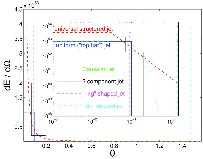
Figure 1: A schematic diagram of the energy per solid angle, $\epsilon=dE/d\Omega$, for the various jet structures that are discussed in this paper, shown both in a linear scale (main figure) and in a log-log scale (big inset at the center).

More “exotic” jet structures have also been considered. One example is a jet with a cross section in the shape of a “ring”, sometimes referred to as a “hollow cone” (Eichler & Levinson, 2003; Levinson & Eichler, 2004; Eichler & Levinson, 2004; Lazzati & Begelman, 2005), which is uniform within $\theta_{c}<\theta<\theta_{c}+\Delta\theta$ where $\Delta\theta\ll\theta_{c}$. Another example is a “fan” or “sheet” shaped jet (Thompson, 2004) where a magneto-centrifugally launched wind from the proto-neutron star, formed during the supernova explosion in the massive star progenitor becomes relativistic as the density in its immediate vicinity drops, and is envisioned to form a thin sheath of relativistic outflow which is somehow able to penetrate through the progenitor star along the rotational equator, forming a relativistic outflow within $\Delta\theta\ll 1$ around $\theta=\pi/2$ (or $\theta_{c}=\pi/2-\Delta\theta/2$). We stress that this has been suggested as a possible jet structure within this model, but the final jet structure is by no means clear, and other jet structure might also be possible within this model (T. A. Thompson, private communication). The various jet structures are shown schematically in Fig. 1.

The light curves for the more conventional jet structures, namely the UJ and USJ models as well as the Gaussian jet model, have been calculated in detail. The light curves for the less conventional jet structures, however, have either been calculated using a simple analytic or semi analytic model (for the two-component jet model), or have not been considered at all (for the “ring” of “fan” jet structures). In this paper we calculate the afterglow light curves for these models. In §2 a simple formalism is developed for calculating the observed emission from a thin spherical relativistic shell, which includes integration over the surface of equal arrival time of photons to the observer. It is generalized to a uniform ring shaped jet, where a finite range in $\theta$ ($\theta_{c}<\theta<\theta_{c}+\Delta\theta$) is occupied by the outflow, in §3. The final expression for the observed flux for any viewing angle is in the form of a sum of two one dimensional integrals, which is trivial to evaluate numerically. This formalism is used to calculate the light curves for various jet structures in §4. In §4.1 it is applied to a uniform jet and a two component jet, while in §§4.2 and 4.3 it is used to calculate the light curves for a ring shaped jet and a fan shaped jet, respectively. Our conclusions are discussed in §5.

2 Calculating the Light Curve from a Relativistic Spherical thin Shell

The emitting shell is assumed to be relativistic, with a Lorentz factor $\gamma=(1-\beta^{2})^{-1/2}\gg 1$, and infinitely thin, so that its location is described by its radius $R$ as a function of the lab frame time $t$. The thin shell approximation is valid in the limit where the width of the shell is $\Delta R\ll R/\gamma^{2}$. Typically, $\Delta R\sim R/\gamma^{2}$ so that the thin shell approximation is only marginally valid, and an integration over the radial profile of the shell might introduce some changes of order unity to the resulting light curve (e.g., Granot, Piran & Sari, 1999; Granot & Sari, 2002). In this work, however, we neglect the radial structure of the emitting shell for the sake of simplicity, and in order to stress the effects of the jet angular structure.

A photon emitted at a radius $R$, at a lab frame time $t$, and at an angle $\theta$ from the line of sight, reaches the observer at an observed time

$$T=t-R\cos\theta\ .$$ (1)

The radius is given by

$$R=c\int_{0}^{t}d\tilde{t}\beta(\tilde{t})\approx ct-\int_{0}^{R}\frac{d\tilde{R}}{2\gamma^{2}(\tilde{R})}\ ,$$ (2)

where the last expression holds in the relativistic limit ($\gamma\gg 1$). Let us assume a power law external density profile, $\rho_{\rm ext}=AR^{-k}$. The deceleration radius is given by

$$R_{\rm dec}=\left[\frac{(3-k)E_{\rm iso}}{4\pi A\eta^{2}c^{2}}\right]^{1/(3-k)}=\left\{\matrix{2.5\times 10^{16}n_{0}^{-1/3}E_{\rm iso,52}^{1/3}\eta_{2.5}^{-2/3}\;{\rm cm}&\quad&k=0\ ,\cr\cr 1.8\times 10^{13}A_{*}^{-1}E_{\rm iso,52}\eta_{2.5}^{-2}\;{\rm cm}&\quad&k=2\ ,}\right.$$ (3)

where $\eta=10^{2.5}\eta_{2.5}$ is the initial Lorentz factor, $E_{\rm iso}=10^{52}E_{\rm iso,52}$ is the isotropic equivalent energy, $n=n_{0}\;{\rm cm^{-3}}$ is the external density for a uniform external medium ($k=0$) and $A=5\times 10^{11}A_{*}\;{\rm g\;cm^{-1}}$ for a stellar wind environment ($k=2$). The corresponding observed deceleration time is

$$T_{\rm dec}=\frac{R_{\rm dec}}{2c\eta^{2}}=\left\{\matrix{4.2(1+z)n_{0}^{-1/3}E_{\rm iso,52}^{1/3}\eta_{2.5}^{-8/3}\;{\rm s}&\quad&k=0\ ,\cr\cr 3.0\times 10^{-3}(1+z)A_{*}^{-1}E_{\rm iso,52}\eta_{2.5}^{-4}\;{\rm s}&\quad&k=2\ .}\right.$$ (4)

The Lorentz factor as a function of radius is given by

$$\gamma(R)\approx\left\{\matrix{\eta&R<R_{\rm dec}\cr\cr\eta(R/R_{\rm dec})^{-(3-k)/2}&R>R_{\rm dec}}\right.\ ,$$ (5)

(Blandford & McKee, 1976). If the bulk velocity of the emitting fluid is in the radial direction, as we assume here, then the flux density is given by

$$F_{\nu}(T) = \frac{(1+z)}{d_{L}^{2}(z)}\int d^{4}x\,\,\delta\left(t-\frac{T}{1+z}-\frac{R\cos\theta}{c}\right)\frac{j^{\prime}_{\nu^{\prime}}}{\gamma^{2}(1-\beta\cos\theta)^{2}}$$

$$= \frac{(1+z)}{4\pi d_{L}^{2}(z)}\int dt\,\,\delta\left(t-\frac{T}{1+z}-\frac{R\cos\theta}{c}\right)\int\frac{dL^{\prime}_{\nu^{\prime}}}{\gamma^{3}(1-\beta\cos\theta)^{3}}\ ,$$

where primed quantities are measured in the local rest frame of the emitting fluid, $j^{\prime}_{\nu^{\prime}}$ is the spectral emissivity (emitted energy per unit volume, frequency, time and solid angle), $L^{\prime}_{\nu^{\prime}}$ is in the spectral luminosity (the total emitted energy per unit time and frequency, assuming a spherical emitting shell), $z$ and $d_{L}(z)=10^{28}d_{L28}\;$cm are the redshift and luminosity distance of the source, respectively, and $\nu^{\prime}=(1+z)\gamma(1-\beta\cos\theta)\nu$. We have $dL^{\prime}_{\nu^{\prime}}=L^{\prime}_{\nu^{\prime}}(R)d\phi d\cos\theta/4\pi$ where $L^{\prime}_{\nu^{\prime}}(R)\propto R^{a}(\nu^{\prime})^{b}$ and the values of the power law indexes $a$ and $b$ depend on the power law segment of the spectrum (Sari, 1998), and are calculate explicitly below.

For simplicity we ignore the self absorption frequency, and assume that the spectrum at any given time is described by three power law segments that are divided by two break frequencies, $\nu_{m}$ and $\nu_{c}$ (Sari, Piran & Narayan, 1998). We also consider only the emission from the shocked external medium, and do not take into account the emission from the reverse shock. Now, $L^{\prime}_{\nu^{\prime},{\rm max}}\propto B^{\prime}N_{e}$, where $B^{\prime}\propto\gamma\rho_{\rm ext}^{1/2}$ is the magnetic field (which is assumed to hold a constant fraction, $\epsilon_{B}$, of the internal energy in the shocked matter), and $N_{e}\propto R^{3-k}$ is the total number of emitting electrons behind the forward shock. Also, $\nu^{\prime}_{m}\propto B^{\prime}\gamma_{m}^{2}\propto B^{\prime}\gamma^{2}$ and $\nu^{\prime}_{c}\propto B^{\prime}\gamma_{c}^{2}\propto\gamma^{-1}R^{3k/2-2}$, which imply

$$L^{\prime}_{\nu^{\prime},{\rm max}} \propto \left\{\matrix{R^{3-3k/2}&R<R_{\rm dec}\cr R^{3/2-k}&R>R_{\rm dec}}\right.\ ,$$ (7)

$$\nu^{\prime}_{m} \propto \left\{\matrix{R^{-k/2}&R<R_{\rm dec}\cr R^{-(9-2k)/2}&R>R_{\rm dec}}\right.\ ,$$ (8)

$$\nu^{\prime}_{c} \propto \left\{\matrix{R^{3k/2-2}&R<R_{\rm dec}\cr R^{k-1/2}&R>R_{\rm dec}}\right.\ .$$ (9)

For fast cooling ($\nu_{c}<\nu_{m}$) we find

$$L^{\prime}_{\nu^{\prime}}(R<R_{\rm dec}) \propto \left\{\matrix{R^{11/3-2k}(\nu^{\prime})^{1/3}&\nu^{\prime}<\nu^{\prime}_{c}\cr R^{2-3k/4}(\nu^{\prime})^{-1/2}&\nu^{\prime}_{c}<\nu^{\prime}<\nu^{\prime}_{m}\cr R^{2-k(p+2)/4}(\nu^{\prime})^{-p/2}&\nu^{\prime}>\nu^{\prime}_{m}}\right.\ ,$$ (10)

$$L^{\prime}_{\nu^{\prime}}(R>R_{\rm dec}) \propto \left\{\matrix{R^{(5-4k)/3}(\nu^{\prime})^{1/3}&\nu^{\prime}<\nu^{\prime}_{c}\cr R^{(5-2k)/4}(\nu^{\prime})^{-1/2}&\nu^{\prime}_{c}<\nu^{\prime}<\nu^{\prime}_{m}\cr R^{[14-9p+2k(p-2)]/4}(\nu^{\prime})^{-p/2}&\nu^{\prime}>\nu^{\prime}_{m}}\right.\ ,$$ (11)

while for slow cooling ($\nu_{c}>\nu_{m}$) we have

$$L^{\prime}_{\nu^{\prime}}(R<R_{\rm dec}) \propto \left\{\matrix{R^{3-k/2}(\nu^{\prime})^{1/3}&\nu^{\prime}<\nu^{\prime}_{m}\cr R^{3-k(p+5)/4}(\nu^{\prime})^{(1-p)/2}&\nu^{\prime}_{m}<\nu^{\prime}<\nu^{\prime}_{c}\cr R^{2-k(p+2)/4}(\nu^{\prime})^{-p/2}&\nu^{\prime}>\nu^{\prime}_{c}}\right.\ ,$$ (12)

$$L^{\prime}_{\nu^{\prime}}(R>R_{\rm dec}) \propto \left\{\matrix{R^{3-4k/3}(\nu^{\prime})^{1/3}&\nu^{\prime}<\nu^{\prime}_{m}\cr R^{[15-9p-2k(3-p)]/4}(\nu^{\prime})^{(1-p)/2}&\nu^{\prime}_{m}<\nu^{\prime}<\nu^{\prime}_{c}\cr R^{[14-9p+2k(p-2)]/4}(\nu^{\prime})^{-p/2}&\nu^{\prime}>\nu^{\prime}_{c}}\right.\ ,$$ (13)

where $p$ is the power law index of the electron energy distribution. The values of $a$ and $b$ that are defined by $L^{\prime}_{\nu^{\prime}}(R)\propto R^{a}(\nu^{\prime})^{b}$ are given in Table 1. The value of $a$ changes at radii corresponding to hydrodynamic transitions, such as $R_{\rm dec}$, where the ejecta stops coasting and starts to decelerate significantly. If there is significant lateral spreading at $R_{j}$ (the radius associated with the jet break time, $T_{j}$, in the afterglow light curve) then this would cause a change in the value of $a$ between $R_{\rm dec}<R<R_{j}$ and $R_{j}<R<R_{\rm NR}$. A similar change in the value of $a$ occurs at the radius of the non-relativistic transition, $R_{\rm NR}$. In this work, however, we concentrate on the relativistic regime ($\gamma\gg 1$ and $R\ll R_{\rm NR}$).

3 Calculating the Light Curves from a Jet with a Uniform Ring Angular Profile

We now specify for a jet with an angular profile of a uniform ring, with an inner half-opening angle $\theta_{c}$ and an angular width $\Delta\theta$,

$$\epsilon=\frac{dE}{d\Omega}=\left\{\matrix{\epsilon_{0}&\theta_{c}<\tilde{\theta}<\theta_{c}+\Delta\theta\cr\cr 0&{\rm otherwise}}\right.\ ,$$ (14)

where $\tilde{\theta}$ is the angle from the symmetry axis of the jet, which is located at an angle $\theta_{\rm obs}$ from the line of sight. Assuming a double sided jet, the true energy is $E=4\pi[\cos\theta_{c}-\cos(\theta_{c}+\Delta\theta)]\epsilon_{0}\approx 2\pi\Delta\theta(2\theta_{c}+\Delta\theta)\epsilon_{0}\approx 4\pi\theta_{c}\Delta\theta\epsilon_{0}$, where the second (third) equality holds in the limit $\theta_{c},\Delta\theta\ll 1$ ($\Delta\theta\ll\theta_{c}$).

We note that this jet structure can be used to describe not only a “ring” shaped jet, but also a uniform jet with sharp edges, a two component jet, or a “fan” shaped jet. A uniform jet of half-opening angle $\theta_{j}$ corresponds to $\theta_{c}=0$ and $\Delta\theta=\theta_{j}$. A two component jet with a narrow (wide) jet component of half-opening angle $\theta_{n}$ ($\theta_{w}$) corresponds to the sum of two rings, the first a uniform jet with $\theta_{c}=0$ and $\Delta\theta=\theta_{n}$ and the second a ring with $\theta_{c}=\theta_{n}$ and $\Delta\theta=\theta_{w}-\theta_{n}$. A “fan” shaped jet corresponds to the limit of a very thin ring, $\Delta\theta\ll\theta_{c}$, as long as $\gamma\theta_{c}\gg 1$, i.e. as long as the visible region of angle $\sim\gamma^{-1}$ around the line of sight is small compared to the half-opening angle of the ring. It can also be directly modeled by $\theta_{c}=\pi/2-\Delta\theta/2$ with $\Delta\theta\ll 1$.

For simplicity, we neglect the lateral spreading of the jet. This is also motivated by the results of numerical studies (Granot et al., 2001; Kumar & Granot, 2003) which show a very modest degree of lateral expansion as long as the jet is sufficiently relativistic.

For a given observed time $T$, $R$ is a function of $\theta$ alone, according to Eq. 1, and does not depend on the azimuthal angle $\phi$. This also applies, within the jet itself, to all the physical quantities in the integrand in Eq. 28, that are a function of $R$: $L^{\prime}_{\nu^{\prime}}(R)$, $\gamma(R)$ and $\beta(R)$. Outside of the jet, however, there is no contribution to the flux. Therefore, we need to determine the fraction, $\Delta\phi/2\pi$, of a circle of angle $\theta$ from the line of sight which intersects the emitting ring, and multiply the integrand in Eq. 28 by this factor. It is most convenient to work in spherical coordinates where the z-axis points to the observer, and the jet axis is within the x-z plane (i.e. at $\phi=0$). The intersection of a cone of half-opening angle $\theta$ around the line of sight with the inner and outer edges of the ring shaped jet occurs at $\phi_{1}$ and $\phi_{2}$, respectively, which are given by

$$\cos\phi_{1} = \frac{\cos\theta_{c}-\cos\theta_{\rm obs}\cos\theta}{\sin\theta_{\rm obs}\sin\theta}\approx\frac{\theta_{\rm obs}^{2}+\theta^{2}-\theta_{c}^{2}}{2\theta_{\rm obs}\theta}\ ,$$ (15)

$$\cos\phi_{2} = \frac{\cos(\theta_{c}+\Delta\theta)-\cos\theta_{\rm obs}\cos\theta}{\sin\theta_{\rm obs}\sin\theta}\approx\frac{\theta_{\rm obs}^{2}+\theta^{2}-(\theta_{c}+\Delta\theta)^{2}}{2\theta_{\rm obs}\theta}\ ,$$ (16)

where the second expression approximately hold when all relevant angles ($\theta_{c}$, $\Delta\theta$, $\theta_{\rm obs}$, $\theta$) are $\ll 1$. We find

$$\frac{\Delta\phi}{2\pi}(\theta_{\rm obs}=0)=\left\{\matrix{1&\theta_{c}<\theta<\theta_{c}+\Delta\theta\cr\cr 0&{\rm otherwise}}\right.\ ,$$ (17)

$$\frac{\Delta\phi}{2\pi}\left(0<\theta_{\rm obs}<\frac{\Delta\theta}{2}\right)=\left\{\matrix{0&\theta<\theta_{c}-\theta_{\rm obs}\cr\cr 1-\phi_{1}/\pi&\theta_{c}-\theta_{\rm obs}<\theta<\theta_{c}+\theta_{\rm obs}\cr\cr 1&\theta_{c}+\theta_{\rm obs}<\theta<\theta_{c}+\Delta\theta-\theta_{\rm obs}\cr\cr\phi_{2}/\pi\ \ &\theta_{c}+\Delta\theta-\theta_{\rm obs}<\theta_{c}+\Delta\theta+\theta_{\rm obs}\cr\cr 0&\theta>\theta_{c}+\Delta\theta+\theta_{\rm obs}}\right.\ ,$$ (18)

$$\frac{\Delta\phi}{2\pi}\left(\frac{\Delta\theta}{2}<\theta_{\rm obs}<\theta_{c}\right)=\left\{\matrix{0&\theta<\theta_{c}-\theta_{\rm obs}\cr\cr 1-\phi_{1}/\pi&\theta_{c}-\theta_{\rm obs}<\theta<\theta_{c}+\Delta\theta-\theta_{\rm obs}\cr\cr(\phi_{2}-\phi_{1})/\pi\ \ &\theta_{c}+\Delta\theta-\theta_{\rm obs}<\theta<\theta_{c}+\theta_{\rm obs}\cr\cr\phi_{2}/\pi\ \ &\theta_{c}+\theta_{\rm obs}<\theta<\theta_{c}+\Delta\theta+\theta_{\rm obs}\cr\cr 0&\theta>\theta_{c}+\Delta\theta+\theta_{\rm obs}}\right.\ ,$$ (19)

$$\frac{\Delta\phi}{2\pi}\left(\theta_{c}<\theta_{\rm obs}<\theta_{c}+\frac{\Delta\theta}{2}\right)=\left\{\matrix{1&\theta<\theta_{\rm obs}-\theta_{c}\cr\cr 1-\phi_{1}/\pi&\theta_{\rm obs}-\theta_{c}<\theta<\theta_{c}+\Delta\theta-\theta_{\rm obs}\cr\cr(\phi_{2}-\phi_{1})/\pi&\theta_{c}+\Delta\theta-\theta_{\rm obs}<\theta<\theta_{c}+\theta_{\rm obs}\cr\cr\phi_{2}/\pi\ \ &\theta_{c}+\theta_{\rm obs}<\theta<\theta_{c}+\Delta\theta+\theta_{\rm obs}\cr\cr 0&\theta>\theta_{c}+\Delta\theta+\theta_{\rm obs}}\right.\ ,$$ (20)

$$\frac{\Delta\phi}{2\pi}\left(\theta_{c}+\frac{\Delta\theta}{2}<\theta_{\rm obs}<\theta_{c}+\Delta\theta\right)=\left\{\matrix{1&\theta<\theta_{c}+\Delta\theta-\theta_{\rm obs}\cr\cr\phi_{2}/\pi&\theta_{c}+\Delta\theta-\theta_{\rm obs}<\theta<\theta_{\rm obs}-\theta_{c}\cr\cr(\phi_{2}-\phi_{1})/\pi&\theta_{\rm obs}-\theta_{c}<\theta<\theta_{c}+\theta_{\rm obs}\cr\cr\phi_{2}/\pi&\theta_{c}+\theta_{\rm obs}<\theta<\theta_{c}+\Delta\theta+\theta_{\rm obs}\cr\cr 0&\theta>\theta_{c}+\Delta\theta+\theta_{\rm obs}}\right.\ ,$$ (21)

$$\frac{\Delta\phi}{2\pi}\left(\theta_{\rm obs}>\theta_{c}+\Delta\theta\right)=\left\{\matrix{0&\theta<\theta_{\rm obs}-\theta_{c}-\Delta\theta\cr\cr\phi_{2}/\pi&\theta_{\rm obs}-\theta_{c}-\Delta\theta<\theta<\theta_{\rm obs}-\theta_{c}\cr\cr(\phi_{2}-\phi_{1})/\pi&\theta_{\rm obs}-\theta_{c}<\theta<\theta_{c}+\theta_{\rm obs}\cr\cr\phi_{2}/\pi&\theta_{c}+\theta_{\rm obs}<\theta<\theta_{c}+\Delta\theta+\theta_{\rm obs}\cr\cr 0&\theta>\theta_{c}+\Delta\theta+\theta_{\rm obs}}\right.\ .$$ (22)

It is more convenient to integrate over $R$, instead of over $\theta$. In the relativistic limit,

$$T\approx\left\{\matrix{\frac{R}{2\eta^{2}c}(1+\eta^{2}\theta^{2})&R<R_{\rm dec}\cr\cr\frac{R}{2\gamma^{2}c}\left[\frac{1}{(4-k)}+\gamma^{2}\theta^{2}\right]+\left(\frac{3-k}{4-k}\right)\frac{R_{\rm dec}}{2\eta^{2}c}=&\cr\frac{R_{L}}{2(4-k)\gamma_{L}^{2}c}\left[(4-k)\gamma_{L}^{2}\theta^{2}x+x^{4-k}+(3-k)x_{\rm dec}^{4-k}\right]&R>R_{\rm dec}}\right.\ ,$$ (23)

where $\gamma_{L}=\gamma(R_{L})$ and $R_{L}(T)$ are the Lorentz factor and radius from which a photon emitted along the line of sight (at $\theta=0$) reaches the observer at an observed time $T$, while $x\equiv R/R_{L}$, and $x_{\rm dec}\equiv R_{\rm dec}/R_{L}$. We have

$$R_{L}(T) = \left\{\matrix{2\eta^{2}c\,T&T<T_{\rm dec}\cr\cr\frac{2(4-k)\gamma_{L}^{2}cT}{1+(3-k)x_{\rm dec}^{4-k}}&T>T_{\rm dec}}\right.\ ,$$ (24)

$$x_{\rm dec} = [(4-k)T/T_{\rm dec}-(3-k)]^{-1/(4-k)}\ ,$$ (25)

and thus obtain

$$\theta^{2}=\left\{\matrix{\frac{1}{\eta^{2}}\left(\frac{2\eta^{2}c\,T}{R}-1\right)&R<R_{\rm dec}\cr\cr\frac{1}{(4-k)\gamma_{L}^{2}}(x^{-1}-x^{3-k})&R>R_{\rm dec}}\right.\ .$$ (26)

Therefore, $d\cos\theta\approx d(\theta^{2})/2=dR[d(\theta^{2})/dR]/2$ where

$$\frac{d\cos\theta}{dx}\approx\frac{R_{L}}{2}\frac{d(\theta^{2})}{dR}=\left\{\matrix{-(cT/R_{L})x^{-2}&x<x_{\rm dec}\cr\cr-\frac{x^{-2}+(3-k)x^{2-k}}{2(4-k)\gamma_{L}^{2}}&x>x_{\rm dec}}\right.\ .$$ (27)

Finally, we can express the integral for the flux density as

$$F_{\nu}(T) = \frac{1}{4\pi D^{2}}\int\frac{dL^{\prime}_{\nu^{\prime}}}{\gamma^{3}(1-\beta\cos\theta)^{3}}$$ (28)

$$= \frac{1}{8\pi D^{2}}\int_{0}^{R_{L}(T)}dR\,\left|\frac{d\cos\theta}{dR}\right|\delta^{3}(R)L^{\prime}_{\nu^{\prime}}(R)\frac{\Delta\phi[\theta(R)]}{2\pi}$$

$$= \frac{1}{8\pi D^{2}}\int_{0}^{1}dx\,\left|\frac{d\cos\theta}{dx}\right|\delta^{3}L^{\prime}_{\nu^{\prime}}\left(\frac{\Delta\phi}{2\pi}\right)\ ,$$

where $\delta\equiv\nu/\nu^{\prime}=1/\gamma(1-\beta\cos\theta)\approx 2\gamma/(1+\gamma^{2}\theta^{2})$ is the Doppler factor, which is given by

$$\delta=\left\{\matrix{(R_{L}/\eta cT)x&x<x_{\rm dec}\cr\cr\frac{2(4-k)\gamma_{L}x^{(k-3)/2}}{4-k+x^{k-4}-1}&x>x_{\rm dec}}\right.\ .$$ (29)

For $T<T_{\rm dec}$ we have $R_{L}=2\eta^{2}cT<2\eta^{2}cT_{\rm dec}=R_{\rm dec}$, and $L^{\prime}_{\nu/\delta}(R)=L^{\prime}_{\nu/2\eta}(R_{L})x^{a}[\delta/2\eta]^{-b}=L^{\prime}_{\nu/2\eta}(R_{L})x^{a-b}$, and therefore

$$F_{\nu}(T)=\frac{2\eta L^{\prime}_{\nu/2\eta}[R_{L}(T)]}{4\pi D^{2}}\int_{0}^{1}dx\,x^{1+a-b}\frac{\Delta\phi(x)}{2\pi}=\frac{2\eta L^{\prime}_{\nu/2\eta}(R_{\rm dec})}{4\pi D^{2}}\left(\frac{T}{T_{\rm dec}}\right)^{a}\int_{0}^{1}dx\,x^{1+a-b}\frac{\Delta\phi(x)}{2\pi}\ .$$ (30)

As long as the outer edge of the ring is not seen, $\Delta\phi/2\pi=1$, and we have a result similar to the spherical case, where $F_{\nu}(T)\propto T^{a}$.

For $T>T_{\rm dec}$ we have $R_{L}(T)>R_{\rm dec}$, and the integral in Eq. 28 naturally divides into two terms, corresponding to $R<R_{\rm dec}$ and $R_{\rm dec}<R<R_{L}$, respectively. Therefore

$$F_{\nu}(T) = \frac{2\eta L^{\prime}_{\nu/2\eta}(R_{\rm dec})}{4\pi D^{2}}\left\{\left(\frac{T}{T_{\rm dec}}\right)^{b-2}\int_{0}^{1}dy\,y^{1+a-b}\frac{\Delta\phi(y)}{2\pi}\right.$$ (31)

$$\quad\quad+\left.x_{\rm dec}^{-a+(1-b)(3-k)/2}\int_{x_{\rm dec}}^{1}dx\,x^{a-2+(3-b)(5-k)/2}\left[\frac{1+(3-k)x^{4-k}}{(4-k)}\right]^{b-2}\frac{\Delta\phi(x)}{2\pi}\right\}\ ,\quad\quad$$

where $y=R/R_{\rm dec}$, and it should be noted that the values of $a$ are generally different in the two integrals. The values of $b$ may also change in the middle of each of the two integrals, in which case this would require to divide the range of integration accordingly, and use the appropriate value of $b$ in each sub-range. From Eq. 31 it can be seen that the second term dominates at $T\gg T_{\rm dec}$, which in the spherical case (where $\Delta\phi/2\pi=1$) implies $F_{\nu}\propto x_{\rm dec}^{-a+(1-b)(3-k)/2}\propto T^{-[-a+(1-b)(3-k)/2]/(4-k)}$, since $x_{\rm dec}\propto 1/R_{L}(T)\propto T^{-1/(4-k)}$.

Please note that $2\eta L^{\prime}_{\nu/2\eta}(R_{\rm dec})=L_{\nu}(R_{\rm dec},\theta=0)$, which means that the coefficient in front of the integrals in Eqs. 30 and 31 is approximately $F_{\nu}(T_{\rm dec})$, for a viewing angle within the jet, which can be calculated from the corresponding values of the peak flux and break frequencies,

$$F_{\rm\nu,max}(T_{\rm dec}) = \left\{\matrix{7.8(1+z)\epsilon_{B,-2}^{1/2}n_{0}^{1/2}E_{\rm iso,52}d_{L28}^{-2}\;{\rm mJy}&\quad&k=0\ ,\cr\cr 2.4\times 10^{5}(1+z)\epsilon_{B,-2}^{1/2}A_{*}^{3/2}\eta_{2.5}^{2}d_{L28}^{-2}\;{\rm mJy}&\quad&k=2\ ,}\right.$$ (32)

$$\nu_{m}(T_{\rm dec}) = \left\{\matrix{4.1\times 10^{18}g^{2}(1+z)^{-1}\epsilon_{B,-2}^{1/2}\epsilon_{e,-1}^{2}n_{0}^{1/2}\eta_{2.5}^{4}\;{\rm Hz}&\quad&k=0\ ,\cr\cr 1.3\times 10^{23}g^{2}(1+z)^{-1}\epsilon_{B,-2}^{1/2}\epsilon_{e,-1}^{2}A_{*}^{3/2}E_{\rm iso,52}^{-1}\eta_{2.5}^{6}d_{L28}^{-2}\;{\rm mJy}&\quad&k=2\ ,}\right.$$ (33)

$$\nu_{c}(T_{\rm dec}) = \left\{\matrix{1.6\times 10^{17}(1+z)^{-1}(1+Y)^{-2}\epsilon_{B,-2}^{-3/2}n_{0}^{-5/6}E_{\rm iso,52}^{-2/3}\eta_{2.5}^{4/3}\;{\rm Hz}&\quad&k=0\ ,\cr\cr 1.1\times 10^{10}(1+z)^{-1}(1+Y)^{-2}\epsilon_{B,-2}^{-3/2}A_{*}^{-5/2}E_{\rm iso,52}\eta_{2.5}^{-2}\;{\rm Hz}&\quad&k=2\ ,}\right.$$ (34)

where $g=3(p-2)/(p-1)$, $Y$ is the Compton y-parameter, and $\epsilon_{e}=0.1\epsilon_{e,-1}$ ($\epsilon_{B}=0.01\epsilon_{B,-1}$) is the fraction of the internal energy behind the shock in relativistic electrons (the magnetic field).

4 Results

4.1 A Two Component Jet

The two component jet model has been suggested as an explanation for sharp rebrightening features in the afterglow light curves of XRF 030723 (Huang et al., 2004) and GRB 030329 (Berger et al., 2003). For XRF 030723, Huang et al. (2004) suggested that our line of sight is slightly outside the wide jet, so that the beaming cone of the radiation from the wide jet expands enough to include the line of sight early on, while that of the narrow jet does so at a significantly later time, causing a bump in the light curve which might account for the sharp bump seen in the optical afterglow light curve of XRF 030723 at $T\sim 15\;$days. In Fig. 2 we show the light curve calculated using the model from §3 with the parameters of the best fit model from Huang et al. (2004), which clearly shows that the resulting bump in the light curve is very smooth due to the integration over the surface of equal arrival time of photons to the observer. Therefore, it cannot produce the very sharp rise in the flux at the onset of the observed rebrightening in the optical afterglow of XRF 030723 (Fynbo et al., 2004). An alternative explanation for this bump in the light curve is a contribution from an underlying supernova component, which naturally produces the red colors that were observed during the bump (Fynbo et al., 2004) and could also potentially produce a sharp enough rise to the bump (Tominaga et al., 2004).

For GRB 030329, Berger et al. (2003) suggested that the sharp bump in the optical afterglow light at $T\sim 1.5\;$days (Lipkin et al., 2004) is due to a two component jet model where our line of sight is within the narrow jet and the bump in the light curve occurs at the deceleration time of the wide jet, $T_{\rm dec,w}$. In Fig. 3 we show the optical light curve for our model from §3 using parameters similar to those used by Berger et al. (2003). Despite the fact that our model assumes an abrupt hydrodynamic transition at the deceleration time, between the early coasting phase and the subsequent self similar deceleration phase, the rise to the bump in the light curve is not sharp enough to match the observations. If a more gradual hydrodynamic transition at $T_{\rm dec,w}$ is assumed, as is shown in Fig. 4 using model 1 of Granot & Kumar (2003), this produces a much smoother bump in the light curve, which is in a much stronger contrast with the observed sharp bump. A much more likely explanation for the bump in the optical light curve of GRB 030329, which can also account for the subsequent bumps in the following days and for the duration of these bumps, is refreshed shocks (Granot, Nakar & Piran, 2003). Thus, we conclude that both a jet viewed off-axis becoming visible and the deceleration of a jet viewed on-axis produce smooth bumps in the afterglow light curves and cannot account for very sharp features.

4.2 A Ring Shaped Jet

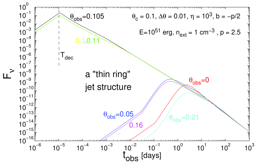
Figure 5: Light curves for a jet with a structure of a thin uniform ring, using the model from §3. The vertical dashed line indicates the deceleration time, $T_{\rm dec}$.

Fig. 5 shows the light curves for a jet with an angular profile of a thin uniform ring, using the model from §3. The jet occupies $\theta_{c}<\theta<\theta_{c}+\Delta\theta$, where in the example shown in Fig. 5, $\theta_{c}=0.1$, $\Delta\theta=0.01$ and $\eta=10^{3}$. For viewing angles within the jet itself, $\theta_{c}\leq\theta_{\rm obs}\leq\theta_{c}+\Delta\theta$, the light curves have a rather small dependence on the exact value of the viewing angle, $\theta_{\rm obs}$. In fact, the light curves for lines of sight at the inner edge ($\theta_{\rm obs}=0.1$; yellow line) and outer edge ($\theta_{\rm obs}=0.11$; green line) of the ring, are practically one on top of the other (making it hard to see the yellow line). The deceleration time occurs early on. The “jet break” in the light curve breaks up into two separate and smaller steepening epochs. The first steepening of the light curve occurs at $T_{j1}$, when both edges of the ring become visible, i.e. when $\gamma\Delta\theta\sim 1$ for a line of sight near the inner or outer edge of the ring, and when $\gamma\Delta\theta\sim 2$ for a line of sight midway across the width of the ring ($\theta_{\rm obs}=\theta_{c}+\Delta\theta/2$). After $T_{j1}$ the light curves from all of the viewing angles within the jet itself ($\theta_{c}\leq\theta_{\rm obs}\leq\theta_{c}+\Delta\theta$) become practically indistinguishable, while before $T_{j1}$ there are small differences, up to a factor of 2. The second steepening of the light curve occurs at $T_{j2}$, when all of the jet becomes visible, i.e. when $\gamma\theta_{c}\sim 1/2$. The light curves from $\theta_{\rm obs}=0$ and $\theta_{\rm obs}=2\theta_{c}+\Delta\theta\approx 2\theta_{c}$ join those for $\theta_{c}\leq\theta_{\rm obs}\leq\theta_{c}+\Delta\theta$ at a slightly earlier time when $\gamma\theta_{c}\sim 1$, while the light curves from $\theta_{\rm obs}=\theta_{c}/2$ or $\theta_{\rm obs}=1.5\theta_{c}+\Delta\theta$ join in earlier on, when $\gamma\theta_{c}\sim 2$. The fact that the jet break is divided into two distinct steepening epoch in the light curve, with half of the total steepening at each epoch, implies that this model cannot reproduce the large steepening at a single jet break time in the light curve as is observed in GRB afterglows. Therefore, this jet structure does not work well for GRB jets.

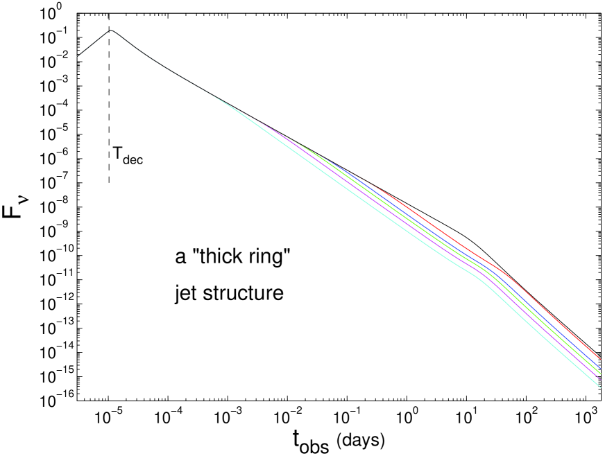
Figure 6: Light curves for a jet with an angular structure of a ring for various fractional widths, viewed from within the jet. The upper line is for a uniform jet viewed from along its symmetry axis ($\theta_{c}=\theta_{\rm obs}=0$, $\Delta\theta=0.2$) and is included for comparison, while the other lines are for a ring shaped jet with $\theta_{c}=0.1$ and $\theta_{c}/\Delta\theta=1,\,2,\,3,\,5,\,10$, from top to bottom, viewed from $\theta_{\rm obs}=\theta_{c}+\Delta\theta/2$. The light curves are calculated using the model from §3, and for a constant energy per solid angle within the jet (corresponding to the same value as in Fig. 5). We also use $k=0$, $n_{0}=1$, $b=-p/2$ and $p=2.5$.

There is, however, a theoretical motivation for a “thick ring” jet structure (Eichler & Levinson, 2003; Levinson & Eichler, 2004; Eichler & Levinson, 2004), where $\theta_{c}/\Delta\theta\sim 2-3$. In Fig. 6 we show the light curves for a line of sight within the jet itself ($\theta_{\rm obs}=\theta_{c}+\Delta\theta/2$) for different values of the ratio $\theta_{c}/\Delta\theta$ which correspond to different fractional widths of the ring. We keep $\theta_{c}=0.1$ and the energy per solid angle within the jet constant, while varying $\theta_{c}/\Delta\theta$. It can be seen that, as expected, $T_{j1}$ is smaller for larger values of $\theta_{c}/\Delta\theta$ which correspond to a narrower ring, while $T_{j2}$ remains roughly constant. We note that even for $\theta_{c}/\Delta\theta$ as low as 1, the two steepening epochs in the light curve, $T_{j1}<T_{j2}$, are still quite distinct and separated by $\sim 1-2$ orders of magnitude in time. For comparison, we also show the light curve for a uniform jet viewed on-axis ($\theta_{c}=\theta_{\rm obs}=0$, $\Delta\theta=0.2$), which produces a single sharp jet break in the afterglow light curve, similar to those observed in GRB afterglows.

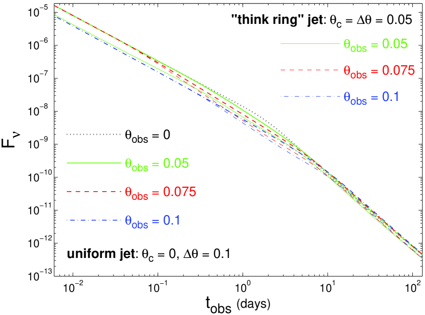
Figure 7: Light curves for a jet with an angular structure of a thick ring compared to those for a uniform conical jet, for different viewing angles. The light curve are calculated using the model from §3 with $k=0$, $n_{0}=1$, $b=-p/2$ and $p=2.5$. The same energy per solid angle is used for the two jet structures.

In Fig. 7 we show the light curves for a “thick ring” jet ($\theta_{c}=\Delta\theta=0.05$) together with those for a uniform conical jet ($\theta_{c}=0$, $\Delta\theta=0.1$) with the same outer angle and the same energy per solid angle, so that the “thick ring” jet is obtained from the uniform conical jet by taking out its inner half (in terms of $\theta$). I can be seen that the light curves for a uniform jet show a sharper jet break for viewing angle near the jet symmetry axis, and somewhat smoother jet breaks for viewing angles closer to the outer edge of the jet. This result is similar to that from numerical simulations (Granot et al., 2001). By comparing the light curves for the two jet structures viewed from the same viewing angle we can see that those for the “thick ring” jet produce a somewhat lower flux as they are missing the contribution from the central part of the jet. The “thick ring” jet also produce a somewhat less pronounced jet break compared to a uniform jet. However, for $\Delta\theta\gtrsim\theta_{c}$ the differences in the light curves compared to those for a uniform conical jet might not be large enough to easily distinguish between these two jet structures using the observed afterglow light curves. Furthermore, for $\Delta\theta\sim\theta_{c}$, if there is relativistic lateral expansion of the jet in its own rest frame, this might help bring $T_{j1}$ and $T_{j2}$ closer together, making the light curves closer to the observations. For $\Delta\theta<\theta_{c}$, however, the effects of lateral spreading should be rather small. We therefore conclude that a ring shaped jet requires a very thick ring, with $\Delta\theta\gtrsim\theta_{c}$, in order to reproduce the observed afterglow light curves, while a jet in the shape of a thinner ring does not produce afterglow light curves with a sharp enough jet break to match afterglow observations.

4.3 A Fan Shaped Jet

An interesting jet structure which resembles a fan can arise due to a magneto-centrifugally launched wind that is driven by the newly formed proto-neutron star during the supernova explosion (Thompson, 2004). If this wind is concentrated within a narrow angle $\theta_{0}$ around the rotational equator and somehow makes it out of the star while still highly relativistic, this could create a GRB outflow within $|\tilde{\theta}|<\theta_{0}$ where $\tilde{\theta}=\theta-\pi/2$ is the angle from the rotational equator (i.e. the latitude). The fraction of the total solid angle that is occupied by such a jet is $f_{b}=\sin\tilde{\theta}_{j}\approx\tilde{\theta}_{j}$. This corresponds to a ring shaped jet with the parameters $\theta_{c}=\pi/2-\Delta\theta/2$ and $\Delta\theta=2\theta_{0}$, using the notations from §3.

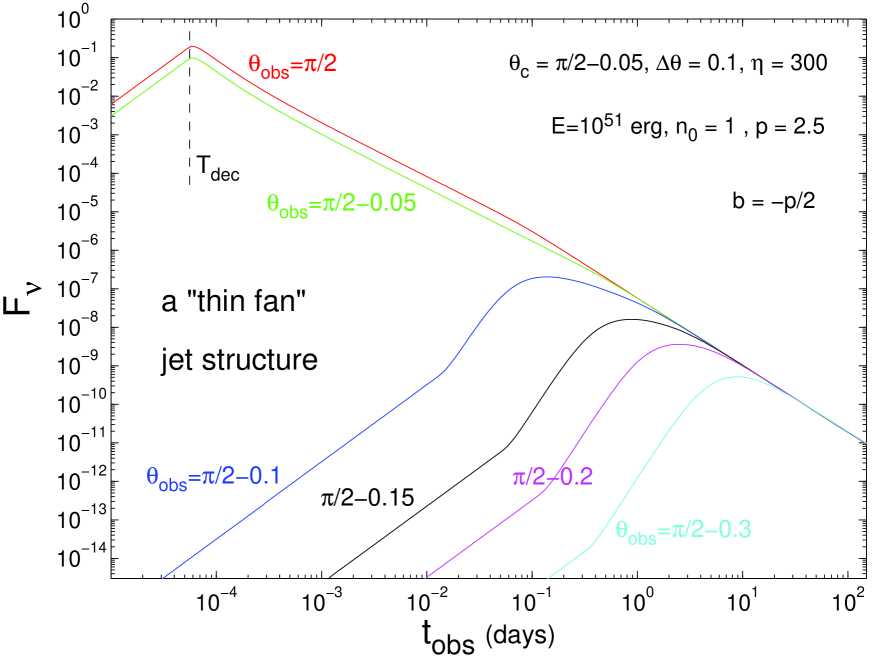
Figure 8: Light curves for a jet with an angular structure of a thin fan, with an opening angle of $\Delta\theta=0.1$ centered on $\theta=\pi/2$ (i.e. $\theta_{c}=\pi/2-\Delta\theta/2=\pi/2-0.05$). The light curves are calculated using the model from §3.

If there is no lateral expansion, then the steepening during the jet break is by a factor of $\sim\gamma\theta_{0}\propto T^{-(3-k)/2(4-k)}$ corresponding to $\Delta\alpha=(3-k)/2(4-k)$ which is $3/8$ for $k=0$ and $1/4$ for $k=2$. This is much shallower than observed in the jet breaks of GRB afterglows, and exactly half as steep (in terms of $\Delta\alpha$) as the jet break for a conical uniform jet. This is demonstrated in Fig. 8 which shows light curves for this jet structure that were calculated using the model from §3. As for the ring shaped jet, the light curves for viewing angles within the jet are similar to each other, differing by up to a factor of 2 before the jet break time, and practically identical after the jet break time. In contrast to the ring shaped jet, there is only one jet break time in the light curve, with at most half the steepening compared to a uniform conical jet. This may be understood as in the limit $\theta_{c}\sim\pi/2$, $T_{j1}$ becomes similar to the time of the non-relativistic transition, and therefore does not produce a distinct break in the light curve, so that the only one epoch of steepening in the light curve remains, at $T_{j1}$, when the edges of the fan shaped jet become visible (i.e. when $\gamma\Delta\theta\sim 1$ for a line of sight at the edge of the jet and when $\gamma\Delta\theta\sim 2$ for a line of sight at the center of the jet). The light curves for lines of sight outside of the jet join those for lines of sight inside the jet when the beaming cone of the radiation from the jet (which extend out to an angle of $\sim 1/\gamma$ form the edges of the jet) reaches the line of sight.

For a relativistic expansion in the local rest frame we have $\tilde{\theta}_{j}\approx\max(\tilde{\theta}_{0},\gamma^{-1})$ so that at $T>T_{j}$, $\tilde{\theta}_{j}\approx\gamma^{-1}$ and

$$E\approx\frac{4\pi}{(3-k)}Ac^{2}R^{3-k}\gamma^{2}\tilde{\theta}\approx\frac{4\pi}{(3-k)}Ac^{2}R^{3-k}\gamma\ ,$$ (35)

implying

$$\gamma\propto R^{k-3}\propto T^{-(3-k)/(7-2k)}\ .$$ (36)

This behavior is intermediate between the spherical case, $\gamma\propto T^{-(3-k)/2(4-k)}$, and the case of a narrow conical jet that expands sideways relativistically in its own rest frame, $\gamma\propto T^{-1/2}$. The temporal decay index at $T>T_{j}$ is also intermediate: $F_{\nu}\propto T^{(12-5k-24p+7kp)/4(7-2k)}$ for $\nu_{m}<\nu<\nu_{c}$ and $F_{\nu}\propto T^{(8-2k-24p+7kp)/4(7-2k)}$ for $\nu>\max(\nu_{c},\nu_{m})$. In both cases $\Delta\alpha$ is reduced by a factor of $(7-2k)/(3-k)$ compared to a uniform conical jet, i.e. the jet break less than half as steep. This result is also valid for the first jet break (at $T_{j1}$) for a a jet in the shape narrow ring, that was discussed in §4.2.

Finally, we have so far assumed that the fan shaped jet occupies all of the range of azimuthal angle $\varphi$. If it occupies a smaller range, $\Delta\varphi<2\pi$, then as long as $\Delta\varphi\gtrsim 1$ the second jet break will overlap with the non-relativistic transition and would not produce a distinct steepening of the light curve. For $\Delta\theta\ll\Delta\varphi\ll 1$, however, there will be two distinct light curves, the first the same as described above and a second jet break when the edges of the jet in the $\varphi$ direction become visible (when $\gamma\Delta\varphi\sim 1$ for a line of sight at the edge of the jet in the $\varphi$ direction, and at $\Delta\varphi\sim 2$ for a line of sight at the center of the jet in the $\varphi$ direction).

5 Conclusions

In §§2 and 3 we have developed a semi-analytic formalism for calculating the the afterglow light curves for a jet with an angular profile of a uniform ring. The final expression for the observed flux is the sum of two one dimensional integrals which are trivial to evaluate numerically. Despite its simplicity, this model includes integration over the surface of equal arrival time of photons to the observer, thus producing realistic results when this is indeed the dominant effect in smoothing out sharp features in the afterglow light curve.

The price of the simple expressions for the observed flux is simple assumptions on the jet dynamics, namely no lateral expansion and an abrupt transition at the deceleration time, $T_{\rm dec}$. This results in a relatively sharp peak in the light curve at $T_{\rm dec}$, while a more realistic model for the dynamics with a smoother dynamical transition at $T_{\rm dec}$ would produce a smoother peak in the light curve (compare Figs. 3 and 4). Nevertheless, when used with care, this simple formalism may serve as a powerful tool. It may also be generalized so that it could be applicable to other jet structures, which were not considered in this work, or to include a calculation of the polarization assuming some local configuration of the magnetic field (e.g., a field tangled within the plane of the shock which is identified with the thin emitting shell).

In §4.1 we have shown that the two-component jet model cannot produce very sharp features in the afterglow light curve, due to the deceleration of the wide (or narrow) jet, or when the narrow (or wide) jet becomes visible at lines of site outside of the jet aperture, as the beaming cone of the emitted radiation reaches the line of sight. Therefore, such explanations for the bumps in the optical light curves of GRB 030329 (Berger et al., 2003) and XRF 030723 (Huang et al., 2004), which both had a sharp rise to the bump, do not work well (see Figs. 2, 3 and 4).

The afterglow light curves for a jet with a ring-like, or “hollow cone” angular profile were calculated in §4.2. We find that the jet break in the light curve divides into two distinct steepening episodes, $T_{j1}$ and $T_{j2}$, with roughly (or in our simple model, exactly) half of the total steepening occurring at each of these two times. The two times remain distinct even for a moderately thick ring, and might merge into a single jet break in the light curve only for a very thick ring, with $\Delta\theta\gtrsim\theta_{c}$.

The light curves for a “fan” shaped jet were calculated in §4.3, and show a single jet break in the light curve with a very moderate steepening across the break, which is at most half of that for a “standard” conical uniform jet. The jet break is even slightly shallower when lateral expansion is taken into account, in which case it is less than half of the steepening for a conical uniform jet. Such a shallow jet break cannot account for the large steepening of the light curves that are observed in GRB afterglows.

Table 1: The Radial Dependence of the Local Rest Frame Spetral Luminosity

PLS	$b$	$a$ ($R<R_{\rm dec}$)	$a$ ($R>R_{\rm dec}$)
D	$1/3$	$3-k/2$	$3-4k/3$
E	$1/3$	$11/3-2k$	$(5-4k)/3$
F	$-1/2$	$2-3k/4$	$(5-2k)/4$
G	$(1-p)/2$	$3-k(p+5)/4$	$[15-9p-2k(3-p)]/4$
H	$-p/2$	$2-k(p+2)/4$	$[14-9p+2k(p-2)]/4$

Note. — The luminosity in the local rest frame of the emitting fluid behind the afterglow shock scales as a power law in frequency and in radius, $L^{\prime}_{\nu^{\prime}}\propto R^{a}(\nu^{\prime})^{b}$, where the power law indexes $a$ and $b$ change between the different power law segments (PLSs) of the spectrum. In addition, $a$ also changes between $R<R_{\rm dec}$ and $R>R_{dec}$. The first column labels the power law segment of the spectrum following the notation of Granot & Sari (2002). The second column provides the value of spectral index $b$, while the third and fourth columns give the value of $a$ for $R<R_{\rm dec}$ and $R>R_{\rm dec}$, respectively.

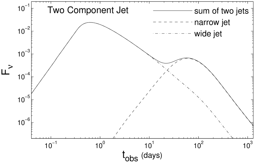
Figure 2: Optical light curve for a two component jet model. The physical parameters of the jet were taken from the best fit model of Huang et al. (2004) to the optical light curve of XRF 030723: $\theta_{n}=0.09$, $\theta_{w}=0.3$, $\theta_{\rm obs}=0.37$, $E_{n,{\rm iso}}=3\times 10^{53}\;$erg, $E_{w,{\rm iso}}=10^{52}\;$erg, $k=0$, $n_{0}=1$ and $p=3.2$. The exact values of $\epsilon_{e}$ and $\epsilon_{B}$ effect the flux normalization but not the shape of the light curve, as long as a break frequency does not pass through the observed frequency band, as is assumed here since we use a constant $b=(1-p)/2$.

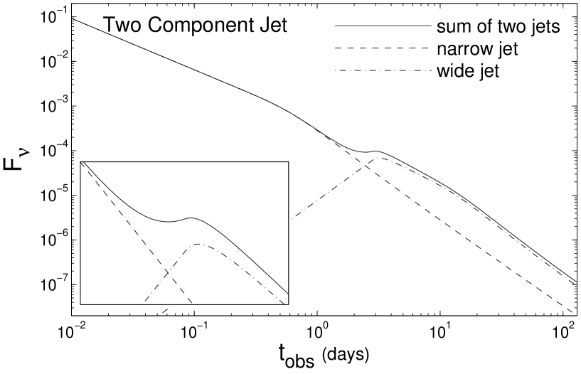
Figure 3: Optical light curve for a two component jet model were the physical parameters of the jet were taken to be similar to those used by Berger et al. (2003) in order to account for the multi frequency afterglow light curves of GRB 030329, namely $\theta_{n}=0.09$, $\theta_{w}=0.3$, $\theta_{\rm obs}=0$, $E_{n,{\rm iso}}=1.2\times 10^{52}\;$erg, $E_{w,{\rm iso}}=5.6\times 10^{51}\;$erg, $\eta_{w}=6.5$, $k=0$, $n_{0}=1.8$, $p=2.2$ and $b=-p/2$. The inset shows a close up of the bump in the light curve that occurs near the deceleration time of the wide jet, as its emission starts to dominate the observed flux.

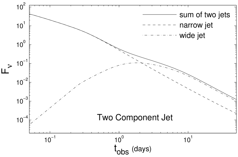
Figure 4: Similar to Fig. 3 but using a different numerical code (model 1 of Granot & Kumar, 2003) which features a more gradual dynamical transition at the deceleration time, resulting in a much smoother bump in the light curve near $T_{\rm dec,w}$.

References

- Berger et al. (2003) Berger, E., et al. 2003, Nature, 426, 154
- Blandford & McKee (1976) Blandford, R.D., & McKee, C. 1976, Phys. Fluids., 19, 1130
- Bloom, Frail & Kulkarni (2003) Bloom, J. S., Frail, D. A., & Kulkarni, S. R. 2003, ApJ, 594, 674
- Costa et al. (1997) Costa, E., et al. 1997, Nature, 387, 783
- Eichler & Levinson (2003) Eichler, D., & Levinson, A. 2003, ApJ, 596, L147
- Eichler & Levinson (2004) Eichler, D., & Levinson, A. 2004, ApJ, 614, L13
- Frail et al. (1997) Frail, D. A., et al. 1997, Nature, 389, 261
- Frail et al. (2000) Frail, D. A., et al. 2001, ApJ, 538, L129
- Frail et al. (2001) Frail, D. A., et al. 2001, ApJ, 562, L55
- Fynbo et al. (2004) Fynbo, J. P. U., et al. 2004, ApJ, 609, 962
- Granot & Kumar (2003) Granot, J., & Kumar, P. 2003, ApJ, 591, 1086
- Granot, Nakar & Piran (2003) Granot, J., Nakar, E., & Piran, T. 2003, Nature, 426, 138
- Granot, Piran & Sari (1999) Granot, J., Piran, T., & Sari, R. 1999, ApJ, 513, 679
- Granot & Sari (2002) Granot, J., & Sari, R. 2002, ApJ, 568, 820
- Granot et al. (2001) Granot, J., Miller, M., Piran, T., Suen, W. M., & Hughes, P. A. 2001, in GRBs in the Afterglow Era, ed. E. costa, F. Frontera, & J. Hjorth (Berlin: Springer), 312
- Granot et al. (2002) Granot, J., Panaitescu, A., Kumar, P., & Woosley, S.E. 2002, ApJ, 570, L61
- Granot, Ramirez-Ruiz & Perna (2005) Granot, J., Ramirez-Ruiz, E., & Perna, R. 2005, submitted to ApJ (astro-ph/0502300)
- Guetta, Granot & Begelman (2005) Guetta, D., Granot, J., & Begelman, M. C. 2005, ApJ, 622, 482
- Huang et al. (2004) Huang, Y. F., Wu, X. F., Dai, Z. G., Ma, H. T., & Lu, T. 2004, ApJ, 605, 300
- Kumar & Granot (2003) Kumar, P., & Granot, J. 2003, ApJ, 591, 1075
- Kumar & Panaitescu (2000) Kumar, P., & Panaitescu, A. 2000, ApJ, 541, L9
- Lazzati & Begelman (2005) Lazzati, D., & Begelman, M. C. 2005, submitted to ApJL (astro-ph/0502084)
- Levinson & Eichler (2004) Levinson, A., & Eichler, D. 2004, ApJ, 613, 1079
- Lipkin et al. (2004) Lipkin, Y. M., et al. 2004, ApJ, 606, 381
- Lipunov, Postnov & Prokhorov (2001) Lipunov, V. M., Postnov, K. A., & Prokhorov, M. E. 2001, Astron. Rep., 45, 236
- Moderski, Sikora & Bulik (2000) Moderski, R., Sikora, M., & Bulik, T. 2000, ApJ, 529, 151
- Panaitescu & Mészáros (1999) Panaitescu, A., & Mészáros, P. 1999, ApJ, 526, 707
- Pedersen et al. (1998) Pedersen, H., et al. 1998, ApJ, 496, 311
- Peng, Königl & Granot (2005) Peng, F., Königl, A., & Granot, J. 2005, ApJ in press (astro-ph/0410384)
- Ramirez-Ruiz, Celotti & Rees (2002) Ramirez-Ruiz, E., Celotti, A., & Rees, M. J. 2002, MNRAS, 337, 1349
- Rhoads (1997) Rhoads, J. E., 1997, ApJ, 487, L1
- Rhoads (1999) Rhoads, J. E., 1999, ApJ, 525, 737
- Rossi, Lazzati & Rees (2002) Rossi, E., Lazzati, D., & Rees, M. J. 2002, MNRAS, 332, 945
- Sari (1998) Sari, R. 1998, ApJ, 494, L49
- Sari, Piran & Halpern (1999) Sari, R., Piran, T. & Halpern, J. 1999, ApJ, 519, L17
- Sari, Piran & Narayan (1998) Sari, R., Piran, T., & Narayan, R. 1998, ApJ, 497, L17
- Thompson (2004) Thompson, T. A. 2004, in “Gamma-Ray Bursts in the Afterglow Era – 4th Workshop”, Rome, Oct. 2004
- Tominaga et al. (2004) Tominaga, N., et al. 2004, ApJ, 612, L105
- van Paradijs et al. (1997) van Paradijs, J., et al. 1997, Nature, 368, 686
- Vlahakis, Peng & Königl (2003) Vlahakis, N., Peng, F., & Königl, A. 2003, ApJ, 594, L23
- Wu et al. (2005) Wu, X. F., Dai, Z. G., Huang, Y. F., & Lu, T. 2005, MNRAS in press (astro-ph/0412011)
- Zhang et al. (2004) Zhang, B., Dai, X., Lloyd-Ronning, N. M., & Mészáros, P. 2004, ApJ, 601, L119
- Zhang & Mészáros (2002) Zhang, B., & Mészáros, P. 2002, ApJ, 571, 876
- Zhang, Woosley & Heger (2004) Zhang, W., Woosley, S. E., & Heger, A. 2004, ApJ, 608, 365
- Zhang, Woosley & MacFadyen (2003) Zhang, W., Woosley, S. E., & MacFadyen, A. I. 2003, ApJ, 586, 356