Luminosity-Dependent Quasar Lifetimes:
Reconciling the Optical and X-ray Quasar Luminosity Functions

Abstract

We consider implications of our new model of quasar lifetimes and light curves for the quasar luminosity function (LF) at different frequencies and redshifts. In our picture, quasars evolve rapidly and the lifetime depends on both their instantaneous and peak luminosities. The bright end of the LF traces the peak intrinsic quasar activity, but the faint end consists of quasars which are either undergoing exponential growth to much larger masses and luminosities, or are in sub-Eddington quiescent states going into or coming out of a period of peak activity. The “break” in the observed LF corresponds directly to the maximum in the intrinsic distribution of peak luminosities, which falls off at both brighter and fainter luminosities. We study this model using simulations of galaxy mergers which successfully reproduce a wide range of observed quasar phenomena, including the observed column density distribution. By combining quasar lifetimes and the distribution of maximum quasar luminosities determined from the observed hard X-ray LF with the corresponding luminosity and host-system dependent column densities, we produce the expected soft X-ray and B-band LFs. Our predictions agree exceptionally well with the observed LFs at all observed luminosities, over the redshift range considered ($z\leq 1$), without invoking any ad hoc assumptions about an obscured population of sources. Our results also suggest that observed correlations in hard X-ray samples between the obscured fraction of quasars and luminosity can be explained in the context of our model by the expulsion of surrounding gas due to heating from accretion feedback energy as a quasar nears its peak luminosity and final black hole mass.

1. Introduction

The nature and evolution of the luminosity function (LF) of quasars at different redshifts and frequencies has been studied for more than thirty years (e.g., Schmidt, 1968; Schmidt & Green, 1983; Boyle et al., 2000; Miyaji et al., 2000; Ueda et al., 2003, and references therein), but its relationship to the intrinsic properties of individual quasars is not well-understood. Spectral synthesis modeling of the X-ray background (e.g., Comastri et al., 1995; Gilli et al., 1999, 2001) as well as observed differences between hard X-ray and soft X-ray or optical quasar LFs (e.g., Boyle et al., 1998; La Franca et al., 2002; Ueda et al., 2003) imply (and require) a large population of optically obscured quasars. However, unified models of active galactic nuclei (AGN) (e.g., Antonucci, 1993) which invoke geometric forms of obscuration as the dominant source of absorption cannot predict the distribution of column densities or differences between LFs, but rather depend on these observations to determine the modeled form of obscuration. Even when calibrated by observed ratios of obscured to unobscured AGN, such models cannot account for measured quasar lifetimes or the selection-effect dependent differences in observed LFs at different frequencies and redshifts. Furthermore, a growing body of observations imply isotropic or evolution-dependent obscuration which cannot be explained by these simple models alone (e.g., Boroson, 1992; Kuraszkiewicz et al., 2000; Tran, 2003; Page et al., 2004; Barger et al., 2005; Alexander et al., 2005; Stevens et al., 2005).

Previous efforts to interpret the quasar LF have relied on restrictive assumptions about lifetimes and light curves of quasars, supposing, for example, that quasars either have universal lifetimes or that they evolve exponentially with time. Semi-analytical modeling of the LF (e.g., Kauffmann & Haehnelt, 2000; Volonteri et al., 2003; Wyithe & Loeb, 2003) has neglected the obscured quasar population and generally focused on reproducing the observed optical or soft X-ray LF, which not only has a different shape but also under-predicts the total quasar population by an order of magnitude at most redshifts and luminosities.

Recently, we have begun to explore the impact of black hole growth on galaxy formation, using simulations of galaxy mergers (Springel et al., 2005b). Our models reproduce the observed correlation between black hole mass and galaxy velocity dispersion (the $M_{BH}-\sigma$ relation) (Di Matteo et al., 2005), and link the quasar phase of galaxies (Hopkins et al., 2005a, b) to galaxy evolution (Springel et al., 2005a). Furthermore, the simulations predict qualitatively different quasar light curves than have been adopted in previous work (Hopkins et al., 2005a, b). In our picture, the peak, exponential black hole growth is determined by the gas supply over timescales $\sim 10^{8}\,{\rm yr}$, during which the gas inflows powering accretion generate large obscuring column densities. The growth shuts down when significant gas is expelled as it is heated by feedback from black hole accretion, creating a window during which the AGN is observable as an optical quasar for a lifetime $\sim 10^{7}\,$yr, in good agreement with observations, and yielding a significant obscured quasar population (Hopkins et al., 2005a). Hopkins et al. (2005b) analyzed simulations over a range of galaxy masses and found that the quasar light curves and lifetimes are all qualitatively similar, with both the intrinsic and observed quasar lifetimes being strongly decreasing functions of luminosity, with longer lifetimes at all luminosities for higher-mass (higher peak luminosity) systems. Moreover, they found that the resulting distribution of column densities $N_{H}$ depends significantly on the observed luminosity threshold, and agrees remarkably well with observed $N_{H}$ distributions of both optical and X-ray samples once the appropriate selection effects are applied.

In Hopkins et al. (2005c) we discuss the intrinsic distribution of source properties obtained by applying our model to the quasar LF, recognizing the essential and realistic property that the time spent at a given luminosity depends on both that luminosity and the peak luminosity of the quasar (or, equivalently, the final black hole mass or host system properties). This results in a qualitatively different distribution of source properties than that implied by the idealized light curves that have been used earlier.

Here, we combine our model of quasar lifetimes and the resulting distribution of intrinsic source properties with the luminosity and host system-dependent $N_{H}$ distributions described above. With these self-consistent results derived from hydrodynamical simulations, we find that the typical column density distribution is a strong function of the instantaneous luminosity of a quasar, and fit it to simple analytical functions. Using the observed hard X-ray quasar LF to recover the distribution of intrinsic source properties, we then combine our models of quasar lifetimes and the corresponding observed column density distributions to reproduce the expected LF at other frequencies given some absolute magnitude/luminosity limit. We find that our predictions for the optical B-band and soft X-ray LFs agree well with observations in both bands. Thus, our model of quasar evolution, without any assumptions, naturally reproduces differences in the hard X-ray, B-band, and soft X-ray LFs over a range of redshifts.

2. The Simulations

The simulations presented here are the series described in detailed in Hopkins et al. (2005b), performed with GADGET-2 (Springel 2005), a new version of the parallel TreeSPH code GADGET (Springel, Yoshida, & White, 2001) based on a fully conservative formulation (Springel & Hernquist, 2002) of smoothed particle hydrodynamics (SPH), which is required for energy and entropy to be simultaneously conserved when smoothing lengths evolve adaptively (see e.g., Hernquist 1993, O’Shea et al. 2005). Our simulations account for radiative cooling, heating by a UV background (as in Katz et al. 1996b, Davé et al. 1999), and incorporate a sub-resolution model of a multiphase interstellar medium (ISM) to describe star formation and supernova feedback (Springel & Hernquist, 2003). Feedback from supernovae is captured in this sub-resolution model through an effective equation of state for star-forming gas, enabling us to stably evolve disks with arbitrary gas fractions (see, e.g. Springel et al. 2005b; Robertson et al. 2004).

Supermassive black holes (BHs) are represented computationally by “sink” particles that accrete gas at a rate $\dot{M}$ estimated from the local gas density and sound speed using an Eddington-limited prescription based on Bondi-Hoyle-Lyttleton theory. The bolometric luminosity of the black hole is $L_{\rm bol}=\epsilon_{r}\dot{M}c^{2}$, where $\epsilon_{r}=0.1$ is the radiative efficiency. We assume that a small fraction (typical $\approx 5\%$) of $L_{\rm bol}$ couples dynamically to the surrounding gas, and that this feedback is injected into the gas as thermal energy. This fraction is a free parameter, which we determine as in Di Matteo et al. (2005) by matching the observed $M_{\rm BH}-\sigma$ relation. For now, we do not resolve the small-scale dynamics of the gas in the immediate vicinity on the black hole, but assume that the time-averaged accretion rate can be estimated from the gas properties on the scale of our spatial resolution ($\lesssim 30$ pc).

The progenitor galaxies in our merger simulations form a family with virial velocities $V_{vir}=80,113,160,226,{\rm and}\ 320\,{\rm km\,s^{-1}}$. The gas equation of state follows the multi-phase, star-forming structure derived in Springel & Hernquist (2003), resulting in a mass-weighted temperature of star forming gas $\sim 10^{5}{\rm K}$. For each simulation, we generate two stable, isolated disk galaxies, each with an extended dark matter halo with a Hernquist (1990) profile, motivated by cosmological simulations (e.g. Navarro et al. 1996; Busha et al. 2004) and observations of halo properties (e.g. Rines et al. 2000, 2002, 2003, 2004), an exponential disk of gas and stars, and a bulge. The self-similarity of any subset of these models is broken by the scale-dependent physics of cooling, star formation, and black hole accretion. The galaxies have masses $M_{\rm vir}=V_{\rm vir}^{3}/(10GH_{0})$ with the baryonic disk having a mass fraction $m_{\rm d}=0.041$, the bulge $m_{\rm b}=0.0136$, and the rest of the mass in dark matter with a concentration parameter $9.0$. In Hopkins et al. (2005a), we describe our analysis of simulation A3, one of our set with $V_{vir}=160\,{\rm km\,s^{-1}}$, a fiducial choice with a rotation curve and mass similar to the Milky Way. We begin our simulation with pure gas disks, which may better correspond to the high-redshift galaxies in which most quasars are observed.

Each galaxy is initially composed of 168000 dark matter halo particles, 8000 bulge particles, 24000 gas and 24000 stellar disk particles, and one BH particle. We vary the initial seed mass of the black hole to identify any systematic dependence of our results on this choice. In the cases considered, we choose the seed mass to be sufficiently small that its presence will not have an immediate effect. Given the particle numbers employed, the dark matter, gas, and star particles are all of roughly equal mass, and central cusps in the dark matter and bulge profiles are reasonably well resolved (see Fig 2. in Springel et al. 2005b). The galaxies are then set to collide from a zero energy prograde orbit.

3. Column Densities in the Simulations

3.1. Determining Column Densities to the Quasar

We determine the column density between a black hole and a distant observer as follows (Hopkins et al., 2005a, b). We calculate the column density between a black hole and a hypothetical observer from simulation outputs spaced every 10 Myr before and after the merger and every 5 Myr during the merger of each galaxy pair. We generate $\sim 1000$ radial lines-of-sight (rays), each with its origin at the black hole particle location and with directions uniformly spaced in solid angle $d\cos{\theta}\,d\phi$. For each ray, we then begin at the origin, calculate and record the local gas properties using GADGET, and then move a distance along the ray $\Delta r=\eta h_{\rm sml}$, where $\eta\leq 1$ and $h_{\rm sml}$ is the local SPH smoothing length. The process is repeated until a ray is sufficiently far from its origin ($\gtrsim 100$ kpc). The gas properties along a given ray can then be integrated to give the line-of-sight column density and mean metallicity. We test different values of $\eta$ and find that gas properties along a ray converge rapidly and change smoothly for $\eta=0.5$ and smaller. We similarly test different numbers of rays and find that the distribution of line-of-sight properties converges for $\gtrsim 100$ rays.

Given the local gas properties, we use the GADGET multiphase model of the ISM described in Springel & Hernquist (2003) to calculate the local mass fraction in “hot” (diffuse) and “cold” (molecular and HI cloud core) phases of dense gas and, assuming pressure equilibrium between the two phases, we obtain the local density of the hot and cold phase gas and the corresponding volume filling factors. The values obtained correspond roughly to the fiducial values of McKee & Ostriker (1977). A detailed description of the properties of both cold and hot phases of the resulting multiphase structure can be found in Springel & Hernquist (2003), Briefly, cold phase (HI or molecular) clouds, with a temperature $\lesssim 1000\,$K, contain a fraction $\gtrsim 0.9$ of the total gas mass above a critical star-forming density threshold determined by the equilibrium solutions to energy balance equations for injection by supernova feedback and radiative cooling. Given a temperature for the warm, partially ionized component $\sim 8000\,{\rm K}$ (with densities $n_{H,\,{\rm hot}}\sim 0.1\,{\rm cm^{-3}}$, or more accurately $\sim 0.01-0.1\,n_{H,\,{\rm total}}$), determined by pressure equilibrium, we further calculate the neutral fraction of this gas, typically $\sim 0.3-0.5$. We denote the neutral and total column densities as $N_{H\,I}$ and $N_{H}$, respectively. Using only the hot-phase density allows us to place an effective lower limit on the column density along a particular line of sight, as it assumes a ray passes only through the diffuse ISM, with $\gtrsim 90\%$ of the mass of the dense ISM concentrated in cold-phase “clumps.” Given the small volume filling factor ($<0.01$) and cross section of such clouds, we expect that the majority of sightlines will pass only through the “hot-phase” component.

We assume the intrinsic quasar continuum SED follows Marconi et al. (2004), based on optical through hard X-ray observations (e.g., Elvis et al., 1994; George et al., 1998; Vanden Berk et al., 2001; Perola et al., 2002; Telfer et al., 2002; Ueda et al., 2003; Vignali et al., 2003). For the extinction at different frequencies, we consider a gas-to-dust ratio equal to that of the Milky Way, $(A_{B}/N_{H\,I})_{\rm MW}=8.47\times 10^{-22}\,{\rm cm^{2}}$, but scaled by metallicity, $A_{B}/N_{H\,I}=(Z/0.02)(A_{B}/N_{H\,I})_{\rm MW}$, as suggested by observations (e.g., Bouchet et al., 1985), although Hopkins et al. (2005a) note that the resulting difference is small. We use the Small Magellanic Cloud (SMC)-like reddening curve of Pei (1992), again motivated by observations (Hopkins et al., 2004). We calculate extinction in X-ray frequencies (0.03-10 keV) using the photoelectric absorption cross sections of Morrison & McCammon (1983) and non-relativistic Compton scattering cross sections, similarly scaled by metallicity. In estimating the column density for photoelectric X-ray absorption, we ignore the calculated ionized fraction of the gas, as it is expected that the inner-shell electrons which dominate the photoelectric absorption edges will be unaffected in the temperature ranges of interest. We do not perform a full radiative transfer calculation, and therefore do not model scattering or re-processing of radiation by dust in the infrared.

3.2. Column Density Evolution During Black Hole Growth

For each simulation, we consider $N_{H}$ values at all times with bolometric luminosity $L=\epsilon_{r}\dot{M}c^{2}$ in some logarithmic interval, weighted by the total time along all sightlines a given $N_{H}$ is observed. This then gives us a binned distribution $P(N_{H}|L)\,d\log(N_{H})\propto t(\log(N_{H}),\ t(\log(N_{H})+d\log(N_{H})))$. This distribution as a function of (observed) luminosity is shown in detail for our fiducial Milky Way-like simulation ($V_{vir}=160\,{\rm km\,s^{-1}}$) in Figure 3 of Hopkins et al. (2005b), in which we demonstrate that the resulting column density distribution reproduces both the typical column density distribution of hard X-ray selected quasar samples (e.g., Ueda et al., 2003), and that of optically selected samples. In particular, the agreement with the column density distribution from the SDSS as determined in Hopkins et al. (2004) is very good, once similar selection effects are applied.

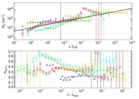
Figure 1.— Lognormal median column density $\bar{N}_{H}$ and dispersion $\sigma_{N_{H}}$ as a function of luminosity and the ratio of instantaneous to peak luminosity, for the simulations described in Hopkins et al. (2005b). Points correspond to quasars with final black hole masses of $7\times 10^{6}\,{\rm(black\ crosses)},\ 3\times 10^{7}\,{\rm(blue\ circles)},\ 1\times 10^{8}\,{\rm(red\ squares)},\ 3\times 10^{8}\,{\rm(cyan\ stars)},\ 7\times 10^{8}\,{\rm(green\ diamonds)},\ {\rm and}\ 2\times 10^{9}\,M_{\sun}{\rm(yellow\ triangles)}$. The black line is the best-fit power law to $\bar{N}_{H}(L)$.

At each intrinsic (un-attenuated) bolometric luminosity $L$ we make a simple approximation to the observed distribution and fit it to a lognormal form,

$$P(N_{H})=\frac{1}{\sigma_{N_{H}}\sqrt{2\pi}}\ \exp[-(\log(N_{H}/\bar{N}_{H})^{2})/(2\sigma_{N_{H}}^{2})].$$ (1)

We show the resulting total (neutral plus ionized) $\bar{N}_{H}$ and $\sigma_{N_{H}}$ for all simulations as a function of $L$ in Figure 1. Although we have shown this for the similar set of simulations described above, we have tested the column density distribution as a function of luminosity across a wide range of simulations, varying the gas fractions, orbital parameters, gas equations of state, concentrations, presence or absence of bulges, and seed black hole masses, and find that, although the final black hole mass (and corresponding peak luminosity) in any of these cases can be dramatically changed, the column density distribution as a function of instantaneous and peak luminosity shows no systematic dependence on any of these host properties (Hopkins et al., in preparation). Therefore we can adopt these fits with reasonable confidence across a wide range of redshifts and luminosities. Indeed, just the simulated luminosities above range from $10^{7}-10^{14}\,L_{\sun}$, covering the entire range of actual observed quasar luminosities at almost all redshifts.

We find that the dependence of $\sigma_{N_{H}}$ on $L$ is weak, and we consider both constant $\sigma_{N_{H}}=0.4$ and a linear best-fit $\sigma_{N_{H}}=0.7+0.1\log{(L/L_{peak})}$. It is important to note, however, that this gives only the dispersion for an individual simulation; in calculating statistical quantities such as the luminosity function, the dispersion across a population is needed. This is easy to determine based on the dispersion in $\bar{N}_{H}$ across simulations. Since we have assumed the distributions are individually lognormal, the dispersion of the quasar population is simply broadened to $\sigma_{N_{H}}\approx 0.8$ (or $\sigma_{N_{H}}=1.0+0.1\log{(L/L_{peak})}$). There is a clear trend of increasing $\bar{N}_{H}$ with $L$, which we fit to a power-law, giving

$$\bar{N}_{H}\approx 4.2\times 10^{21}\,{\rm cm^{-2}}\,(L/10^{11}\,L_{\sun})^{0.35}.$$ (2)

We note that the median neutral column density, $\bar{N}_{H\,I}$, follows a similar relation, with a typical ionized fraction $0.3-0.5$ (mean 0.35). This form can be understood roughly as follows, in the context of buried quasar growth during times when the black hole mass is growing to its final mass, before peak quasar stages. Consider the time-dependent mass $M_{c}$ within the merging core of radius $R_{c}$ ($\sim 100\,{\rm pc}$), and assume that the black hole grows such that $M_{BH}\sim\eta M_{c}$ ($\eta\sim 0.005$) (Magorrian et al., 1998). The total density is then $\rho=M_{c}R_{c}^{-3}f(r)$, where $f(r)$ is a dimensionless profile of order unity, and the column density is $N_{H\,I}=(f_{\ast}M_{c})/(\mu m_{H}R_{c}^{2})$, where $f_{\ast}$ is the product of the mean neutral, hot-phase fraction ($\lesssim 0.01$ in the most dense regions of the galaxy) and the integral of the density profile $f(r)$ ($\sim 1$), and $\mu$ is the mean molecular weight. This gives $N_{H\,I}\approx 10^{21}\,{\rm cm^{-2}}\,m_{8}$, where $M_{c}=m_{8}\times 10^{8}\,M_{\sun}$. The luminosity, from a Bondi accretion model, is $L=\epsilon_{r}\dot{M}c^{2}=4\pi\alpha\epsilon_{r}(GM_{BH})^{2}\rho c^{2}/c_{s}^{3}$, or using the definitions above, $L=(4\pi\alpha\epsilon_{r}\eta^{2}f_{0})(c/c_{s})^{3}(G^{2}M_{c}^{3})/(cR_{c}^{3})$, where $f_{0}=f(r)\sim 1$ as appropriate for some “accretion radius” and $c_{s}$ is the (mass-weighted) sound speed ($\sim 30\,{\rm km/s}$ in the approximately isothermal core). These values give $L\approx 10^{11}\,L_{\sun}\,m_{8}^{3}$. Thus, we expect $N_{H\,I}\sim 10^{21}\,{\rm cm^{-2}}\,(L/10^{11}\,L_{\sun})^{1/3}$, with variation of the above parameters as well as dynamical and feedback effects generating the considerable scatter seen in this relationship. This relation is much shallower than the naively expected relation $N_{H}\propto L$ expected if $M_{BH}$ is constant ($L\propto\rho\propto N_{H}$) or $L\propto M_{BH}$ always, and strongly contrasts with unification models which predict static obscuration or $N_{H}$ independent of $L$ up to some threshold (e.g., Fabian, 1999).

This modeling naturally produces a population of heavily attenuated objects at large luminosities. Although our fitted hot-phase column densities do not reach extremely Compton-thick levels $N_{H}\gtrsim 10^{25-26}\,{\rm cm^{-2}}$, the brightest objects shown in Figure 1 reach median column densities $\sim 10^{23}\,{\rm cm^{-2}}$ or larger. As the fitted distribution is a lognormal about this median with a dispersion across the quasar population $\sigma_{N_{H}}\sim 1$, this implies a significant population of heavily attenuated ($N_{H}\sim 10^{23}-10^{24}\,{\rm cm^{-2}}$) objects at soft X-ray (0.5-2 keV) frequencies; with the number density of sources falling of with larger $N_{H}$. This agrees well with both direct observations (Treister et al., 2004; Mainieri et al., 2005) as well as synthesis models of the X-ray background (Madau et al., 1994; Comastri et al., 1995; Gilli et al., 1999, 2001), which require a population of such objects, suggesting that our model should in principle account for the X-ray background spectrum based on a given luminosity function, without adopting arbitrary distributions of source obscuration or additional obscured populations. Furthermore, as discussed in Hopkins et al. (2005b), extension of this distribution of $N_{H}(L)$ to very bright quasars in unusually massive galaxies or quasars in higher-redshift, compact galaxies which we have not simulated may, during peak accretion periods, reach Compton-thick values ($N_{H}\gtrsim 10^{25}\,{\rm cm^{-2}}$) of the typical column density. More likely, as our model assumes $\sim 90\%$ of the mass of the densest gas is clumped into cold-phase molecular clouds, a small fraction of sightlines will pass through such clouds and encounter column densities similar to those shown for the cold phase in Figure 2 of Hopkins et al. (2005a) and Figures 4 and 5 of Hopkins et al. (2005b), as large as $N_{H}\sim 10^{26}{\rm cm^{-2}}$. This also allows a large concentration of mass in sub-resolution obscuring structures, such as an obscuring toroid on scales $\lesssim 100\,$pc, although many of the phenomena such structures are invoked to explain can be accounted for through our model of time-dependent obscuration. Geometrical effects may therefore, however, become relevant for interpreting and explaining the Compton-thick source population.

3.3. Column Densities in Final Growth Stages

Although the physical motivation for such a dependence is intuitive, the trend of increasing column density with luminosity seems to run opposite to that observed in a number of X-ray samples (Steffen et al., 2003; Ueda et al., 2003; Hasinger, 2004; Grimes, Rawlings, & Willott, 2004; Sazonov & Revnivtsev, 2004; Barger et al., 2005; Simpson, 2005). In these samples, it appears that the fraction of broad-line objects and the fraction below some moderate column density ($N_{H}=10^{22}\,{\rm cm^{-2}}$) increase with luminosity, at odds with our prediction. However, a more detailed inspection reveals that our simulations can and do, in fact, reproduce this behavior. Although it is possible to extend our spectral modeling of the quasar and column density calculation to describe the complete stellar population of the galaxy, and so determine more accurately when an X-ray selected quasar will show a typical broad-line spectrum, we defer this to a later paper as it requires calculating colors and attenuations of the stars at all times in our simulations. However, we can easily compare to the observations of e.g., Ueda et al. (2003), and consider the fraction of objects with $N_{H}<10^{22}\,{\rm cm^{-2}}$ (more accurately, the ratio of number with $N_{H}<10^{22}\,{\rm cm^{-2}}$ to all with $N_{H}<10^{24}\,{\rm cm^{-2}}$) as a function of hard X-ray luminosity.

Figure 2.— The column density distribution at three observed hard X-ray (2-10 keV) luminosities, from the Milky Way like ($V_{vir}=160\,{\rm km\,s^{-1}}$) simulation of Hopkins et al. (2005a), with a peak hard X-ray luminosity $L_{X,\ {\rm peak}}=5\times 10^{44}\,{\rm erg\,s^{-1}}$. The luminosities are chosen to be well below the peak luminosity (upper left) and near peak, corresponding to the final stages of obscured black hole growth (upper right) and subsequent “blowout” phase (lower left) as feedback from accretion energy expels gas in the central regions of the galaxy. Lower right shows the fraction of sightlines with $N_{H}>10^{22}\,{\rm cm^{-2}}$ from the six simulation outputs closest in time and luminosity to $L_{X,\ {\rm peak}}$ (black diamonds), with horizontal errors the spacing in luminosity and vertical errors corresponding to the range across different possible column density prescriptions compared in Hopkins et al. (2005b). Solid line is the best-fit obscured fraction as a function of luminosity from Simpson (2005). Circles show the observations from Ueda et al. (2003), with the dashed line the expectation from their fitted $N_{H}$ function.

We examine the $N_{H}$ distribution of our fiducial, Milky Way-like ($V_{vir}=160\,{\rm km\,s^{-1}}$) simulation in detail in Figure 2. Over most of the simulation, we find the general trend shown in Figure 1 and discussed above. The upper left panel shows the binned column density distribution (arbitrary scale) for all times with an observed hard X-ray luminosity $L^{\rm obs}_{X}(2-10\,{\rm keV})=10^{41}-10^{42}\,{\rm erg\,s^{-1}}$ (we use these units for ease of comparison with the observations quoted above), well below the peak observed hard X-ray quasar luminosity $\approx 5\times 10^{44}\,{\rm erg\,s^{-1}}$, at which point the evolution is following the normal trend shown in Figure 1. However, when the quasar nears its final, peak luminosity, there is a rapid “blowout” phase as thermal feedback from the growing accretion heats the surrounding gas, driving a strong wind and eventually cutting off the accretion process, leaving a remnant with a black hole satisfying the $M_{\rm BH}-\sigma$ relation (Di Matteo et al., 2005; Hopkins et al., 2005a). We analyze this “blowout” phase in some detail in Hopkins et al. (2005a), and find that it can be identified with the traditional bright optical quasar phase, as the final stage of black hole growth with a rapidly declining density (allowing the quasar to be observed in optical samples), giving typical luminosities, column densities, and lifetimes of optical quasars (Hopkins et al., 2005a, b) in good agreement with observations (e.g., Hopkins et al., 2004; Martini, 2004).

If we consider these stages of quasar growth, then, near the peak luminosity, we find a very different trend. The upper right panel of Figure 2 shows the column density distribution for times with $L^{\rm obs}_{X}\approx 10^{44}\,{\rm erg\,s^{-1}}$, primarily in the final stages of the rapid obscured black hole growth phase, just before feedback from the accretion begins to expel the surrounding gas. The typical column densities are large, $\gtrsim 10^{22}\,{\rm cm^{-2}}$, as we expect from our modeling above, although not high enough to generate large extinction in hard X-rays. However, just $\sim 10$ Myr later, the quasar has expelled a significant amount of gas and column densities fall rapidly. The lower left panel of the figure shows the column density distribution for times with a typical luminosity $L^{\rm obs}_{X}\approx 10^{44.5}\,{\rm erg\,s^{-1}}$, essentially the very peak quasar luminosity, corresponding to the bright observable phase in which the quasar is driving a wind and expelling nearby gas. The typical column densities are lower by an order of magnitude, $N_{H}\sim 10^{21}-10^{22}\,{\rm cm^{-2}}$. In the lower right panel of the figure, we plot the fraction of sightlines with column densities above $10^{22}\,{\rm cm^{-2}}$ (the “obscured fraction”), for the six simulation outputs closest (in both time and luminosity) to the peak luminosity of the quasar. The results are shown (black diamonds) with the range in luminosity between each simulation output shown as horizontal error bars. In Hopkins et al. (2005b) we discuss in detail the differences in column densities that result from varying our method of calculation, and find that (after accounting for some hot phase-cold phase separation) adopting various extreme cases yields a factor $\sim 2$ difference in the calculated column densities, so we plot the resulting differences in the obscured fraction from this uncertainty as vertical error bars. The data from Ueda et al. (2003) (circles) and their expectation from their fitted column density distribution (dashed lines) are shown for comparison, as is the best-fit obscured fraction as a function of luminosity from Simpson (2005) (solid line).

The agreement between the observations and our result is encouraging, especially as our calculation considers only one simulation, and is not necessarily meant to reproduce the trend in observed quasar populations. However, we do find a similar trend in all of our simulations near the peak luminosity (see also Hopkins et al., 2005a, b). The key point is that we find, near the peak luminosity of the quasar as feedback drives away gas and shuts down accretion processes, the typical column densities fall rapidly with luminosity in a manner similar to that observed. In our model for the luminosity function, proposed in Hopkins et al. (2005c), quasars below the “break” in the observed luminosity function are either growing efficiently in early stages of growth or in sub-Eddington phases coming into or our of their peak quasar activity. Around and above the break in the luminosity function, the observed luminosity function becomes dominated by sources at high Eddington ratio at or near their peak luminosities. Based on the above calculation, as well as the description of the blowout phase from Hopkins et al. (2005a), we then immediately expect what is observed, that in this range of luminosities, the fraction of objects observed with large column densities will rapidly decrease with luminosity as the observed sample is increasingly dominated by sources at their peak luminosities in this blowout phase. This also further emphasizes that the evolution of quasars dominates over static geometrical effects in determining the observed column density distribution at any given luminosity.

4. Quasar Lifetimes & the Luminosity Function

Hopkins et al. (2005c) showed that a proper accounting of realistic quasar light curves results in luminosity-dependent quasar lifetimes. In this picture, quasar lifetimes are functions of both the instantaneous luminosity and the peak luminosity (i.e. final black hole mass or host galaxy properties) of the system. Given a quasar lifetime above some luminosity as a function of the peak luminosity of the quasar, $t(L^{\prime}>L,L_{peak})$, the quasar LF (in the absence of selection effects) is given by

$$\Phi(L)=\int{\frac{dt(L,L_{peak})}{d\log(L)}\,\dot{n}(L_{peak})}\,d\log(L_{peak}),$$ (3)

where $\dot{n}(L_{peak})$ is the rate at which of sources in a given logarithmic interval in $L_{peak}$ are “born” (created or activated) per unit volume and $\Phi(L)$ is the number density of sources per logarithmic interval in $L$. This formulation implicitly accounts for the “duty cycle” (the fraction of active quasars at a given time), which is proportional to the lifetime at a given luminosity. At any redshift, $\dot{n}(L_{peak})$ will be, in general, a complicated function of the distribution of galaxy properties, including merger rates, masses, and gas fractions. However, having determined the quasar lifetime from our simulations, we can use an observed luminosity function to de-convolve $\dot{n}(L_{peak})$. Since we are only interested here in demonstrating that our modeling self-consistently reproduces the observed differences in luminosity functions, in concert with the interpretation of the luminosity function from Hopkins et al. (2005c), we adopt this semi-empirical approach in what follows, and thus all quantities in the equations determining the intrinsic and observed luminosity functions are completely determined.

Given a distribution of $N_{H}$ values and some minimum observed luminosity $L_{\nu}^{min}$, the fraction $f_{obs}$ of quasars with a peak luminosity $L_{peak}$ and instantaneous bolometric luminosity $L$ which lie above the luminosity threshold is given by the fraction of $N_{H}$ values below a critical $N_{H}^{max}$, where $L_{\nu}^{min}=f_{\nu}L\,\exp{(-\sigma_{\nu}N_{H}^{max})}$. Here, $f_{\nu}(L)\equiv L_{\nu}/L$ is a bolometric correction and $\sigma_{\nu}$ is the cross-section at frequency $\nu$. Thus,

$$N_{H}^{max}(\nu,L,L_{\nu}^{min})=\frac{1}{\sigma_{\nu}}\ln{\Bigl{(}\frac{f_{\nu}(L)L}{L_{\nu}^{min}}\Bigr{)}},$$ (4)

and for the lognormal distribution above,

$$f_{obs}(\nu,L,L_{peak},L_{\nu}^{min})=\frac{1}{2}\Bigl{[}1+{\rm erf}\Bigl{(}\frac{\log{(N_{H}^{max}/\bar{N}_{H})}}{\sqrt{2}\,\sigma_{N_{H}}}\Bigr{)}\Bigr{]}.$$ (5)

This results in a LF (in terms of the bolometric luminosity)

$$\begin{split}\Phi(\nu,L,L_{\nu}^{min})&=\frac{1}{t_{\ast}}\int{f_{obs}(\nu,L,L_{peak},L_{\nu}^{min})}\\ &\quad\times\frac{dt(L,L_{peak})}{d\log(L)}\,\dot{n}(L_{peak})\,d\log(L_{peak}).\end{split}$$ (6)

The important point to recognize in this equation is that $f_{obs}$ has a complicated dependence on both instantaneous and peak luminosity (which does not simply factor out of the above integrals), and thus the equations above will have a non-trivial dependence on the distribution of quasar peak luminosities $\dot{n}(L_{peak})$ and the quasar lifetime, which are very different in our analysis from what has generally been used in previous modeling attempts.

We consider quasar lifetimes determined from the simulations described in Hopkins et al. (2005a, b). The light curves in the mergers are complicated, generally having a period of early rapid accretion after “first passage” of the galaxies, followed by an extended quiescent period, then a transition to a peak, highly luminous quasar phase, and then a dimming as self-regulated mechanisms expel gas from the galaxy center after the black hole reaches a critical mass and shut down accretion (Di Matteo et al., 2005). While complex, Hopkins et al. (2005b) find that the total quasar lifetime $t_{Q}(L^{\prime}>L)$ above a given luminosity $L$ is well-approximated by a truncated power law for every simulation studied, with $t_{Q}(L^{\prime}>L)=t_{9}\,(L/10^{9}\,L_{\sun})^{\alpha}$, where $t_{9}\equiv t_{Q}(L^{\prime}>10^{9}\,L_{\sun})\sim 10^{9}\,{\rm yr}$, over the range $10^{9}\,L_{\sun}<L<L_{peak}$ for a given quasar. Given then that Hopkins et al. (2005b) find this normalization is approximately constant across simulations, the lifetime in each simulation is then entirely determined by the power-law slope $\alpha$. The value of $\alpha$ depends on the peak luminosity of the quasar (equivalently, the final black hole mass or host system properties), with more massive (higher peak luminosity) quasars yielding shallower power-law slopes as they spend more time at high luminosities and large Eddington ratios. Over a wide range of $L_{peak}$ (from $\sim 10^{10}-10^{14}\,L_{\sun}$), Hopkins et al. (2005b) find $\alpha=\alpha(L_{peak})$ is approximately linear with $\log{L_{peak}}$, $\alpha=\alpha_{0}+\alpha^{\prime}\,\log{L_{peak}}$ with an upper limit $\alpha=-0.2$. The time spent in any logarithmic luminosity interval in this range is then simply

$$dt/d\log(L)=|\alpha|\,t_{9}\,(L/10^{9}\,L_{\sun})^{\alpha}.$$ (7)

Hopkins et al. (2005c) examine a series of possible restrictions to this model, which change $\alpha(L_{peak})$ slightly but yield very similar behavior, and we have considered all the cases described therein and obtain identical results in every case using luminosity-dependent quasar lifetimes of this form. We show results for the case in which $\alpha$ is determined from the entire duration of our simulations, without imposing any arbitrary cutoffs, which gives $\alpha_{0}=-0.95$ and $\alpha^{\prime}=0.32$ for $L_{peak}$ in units of $10^{12}\,L_{\sun}$, i.e. $\alpha=-0.95+0.32\log{(L_{peak}/10^{12}L_{\sun})}$.

Given this model of $dt/d\log(L)$ as a function of $L$ and $L_{peak}$, we can then fit to any $\Phi(L)$ to determine $\dot{n}(L_{peak})$. The resulting distributions $\dot{n}(L_{peak})$, discussed in Hopkins et al. (2005c) are fundamentally different from the naive expectation of previous analyses of the LF which relied on idealized models of the quasar lifetime, either assuming quasars “turn on” at a fixed luminosity for some universal lifetime, ($dt/d\log(L)\propto\delta(L-L_{0})$) or assuming a pure exponential light curve over some interval ($dt/d\log(L)={\rm constant}$). These previous models for the quasar lifetime yield a direct relationship between an observed luminosity and peak luminosity (final black hole mass), and predict a distribution of peak luminosities $\dot{n}(L_{peak})$ with essentially identical shape to the observed LF. However, accounting for the luminosity dependence of quasar lifetimes based on our detailed modeling, we find that quasars spend significantly more time at low luminosities than near their peak, resulting in a very different $\dot{n}(L_{peak})$ distribution. In this modeling, $\dot{n}(L_{peak})$ has the same shape as the observed LF above the “break” in the luminosity function, and these quasars are accreting at high efficiency, near their peak luminosities. Below the break luminosity, however, the $\dot{n}(L_{peak})$ distribution turns over, and the faint end of the luminosity function is dominated by sources near the break luminosity (the peak of the $\dot{n}(L_{peak})$ distribution) accreting either at high efficiency but in early stages of merger and growing to much larger luminosities, or in sub-Eddington phases going into or out of peak quasar activity (in the final stages of the host galaxy merger). The evolution of the LF with redshift, then, directly relates to evolution in $\dot{n}(L_{peak})$, with the characteristic peak luminosity of quasars (final black hole mass being built) increasing with redshift as the break luminosity shifts to larger values. It is of particular interest to determine if this modeling of quasar evolution and the consequent novel interpretation of the luminosity function produce differences in the luminosity function in different wavebands (as well as column density distributions) consistent with what is observed. Furthermore, when comparing different models of quasar lifetimes and the luminosity function, even for $\dot{n}(L_{peak})$ distributions chosen such that two different quasar lifetime models will produce an identical luminosity function in a given waveband, any dependence of the column density distribution on peak luminosity (i.e. host system properties) or Eddington ratio will result in a different prediction for the luminosity function at all other frequencies.

Figure 3.— Upper panels: Hard X-ray (thick; Ueda et al., 2003), soft X-ray (thin; Miyaji et al., 2000), and B-band (dot-dash; Boyle et al., 2000) LFs at $z=1.0$, rescaled using the bolometric corrections from Marconi et al. (2004) which we adopt throughout (left) and the luminosity-independent average corrections from Elvis et al. (1994) (right). Lower panels: The ratio of soft X-ray (solid) and B-band (dot-dash) LFs to the hard X-ray LF above. LFs are plotted over the corresponding range of the observed luminosities in the Ueda et al. (2003) hard X-ray LF at this redshift. Vertical lines bracket the minimum and maximum bolometric luminosities for which observational data exist (according to the appropriate bolometric correction) in the soft X-ray (solid line, only a minimum shown) and B-band (dot-dashed lines). Outside of these ranges the fitted luminosity functions are extrapolated beyond the data.

We consider the observed luminosity functions in the hard X-ray ($\Phi_{HX}$; 2-10 keV), soft X-ray ($\Phi_{SX}$; 0.5-2 keV), and optical B-band ($\Phi_{B};\ \lambda_{B}=4400\,$Å), from Ueda et al. (2003); Miyaji et al. (2000); Boyle et al. (2000), respectively. We rescale all luminosity functions to the same $\Omega_{m}=0.3$, $\Omega_{\Lambda}=0.7$, $H_{0}=70\,{\rm km\,s^{-1}\,Mpc^{-1}}$ cosmology. In order to make a direct comparison between luminosity functions, we further rescale all luminosity functions in terms of the bolometric luminosity, using the bolometric corrections of Marconi et al. (2004). It is important to note that using the constant, luminosity-independent bolometric corrections of e.g. Elvis et al. (1994) instead results in a significantly steeper cutoff in the luminosity function at high bolometric luminosities, as the bolometric luminosity inferred for the brightest observed X-ray quasars is almost an order of magnitude smaller using the Elvis et al. (1994) corrections. However, it has been well-established that the ratio of bolometric luminosity to hard or soft X-ray luminosity increases with increasing luminosity (e.g., Wilkes et al., 1994; Green et al., 1995; Vignali et al., 2003; Strateva et al., 2005), and further the sample quasars of Elvis et al. (1994) are X-ray bright (Elvis et al., 2002). Accounting for the luminosity dependence of the UV to X-ray flux ratio, $\alpha_{OX}$, gives rise to most of this difference. We adopt the form for $\alpha_{OX}$ from Vignali et al. (2003), but our results are relatively insensitive to the different values found in the literature. These differences in the resulting bolometric luminosity functions are illustrated in Figure 3. The upper left shows the luminosity functions $\Phi_{HX}$ (thick), $\Phi_{SX}$ (thin), and $\Phi_{B}$ (dashed) at $z=1.0$, with bolometric luminosities from the Marconi et al. (2004) corrections and corresponding densities rescaled according to

$$\frac{d\Phi}{d\log{L}}=\frac{d\Phi}{d\log{L_{\nu}}}\frac{d\log{L_{\nu}}}{d\log{L}}.$$ (8)

This can be compared to the same luminosity functions converted using the constant bolometric corrections of Elvis et al. (1994) (upper right). In both cases the qualitative differences are similar, with the hard X-ray luminosity function significantly above the soft X-ray or optical LF at low luminosities just below the break, and the ratio of hard X-ray to soft X-ray or optical LF decreasing at and just above the break. This is seen in the lower panels of the figure, where we plot the corresponding ratios $\Phi_{SX}/\Phi_{HX}$ (solid) and $\Phi_{B}/\Phi_{HX}$ (dot-dash). However, it is apparent that the inferred number density from the X-ray LFs decreases much more slowly with luminosity using the Marconi et al. (2004) corrections which account for the luminosity dependence of $\alpha_{OX}$, resulting in a larger gap at a given luminosity between the hard and soft X-ray LFs (and the optical as well). It is also immediately clear in this plot that the constant bolometric corrections of Elvis et al. (1994) cannot apply uniformly to all luminosities and redshifts, as this actually predicts a larger number of optically selected bright quasars than soft or hard X-ray objects, which cannot be explained with any sort of reddening/obscuration model. This is not a fitting artifact, as a direct comparison of the data between, e.g., Croom et al. (2004) and Barger et al. (2005) in the optical and hard X-ray, respectively, shows (using the Elvis et al. (1994) corrections) the optical quasar LF to be a factor $\sim 2-3$ higher than the hard X-ray LF at several luminosities and redshifts, and this problem is only worse when considering the optical LFs of Boyle et al. (2000) or Richards et al. (2005) which are steeper at low luminosity than that of Croom et al. (2004). Furthermore, there is direct evidence of a significant number of optically obscured quasars, even at high luminosities (Norman et al., 2002; Stern et al., 2002; Dawson et al., 2003; Treister et al., 2004), many of which are undergoing a buried quasar or pre-quasar growth phase (Page et al., 2004; Alexander et al., 2005; Stevens et al., 2005) as predicted in our modeling. As discussed above, the existence of a significant population of such objects is also inferred from synthesis models of the X-ray background (Madau et al., 1994; Comastri et al., 1995; Gilli et al., 1999, 2001). At the extreme low and high luminosities shown, the relative behavior of the plotted LFs becomes confusing, but this is because they are extrapolated well beyond the range of observed data. Therefore, we show the actual range of observed luminosities for each LF as vertical lines (of the same style as the corresponding LF). The difference in LFs across these ranges are much less dramatic, and this is what we are interested in making a detailed comparison with. It is clear, though, that it is important to account for the luminosity dependence of quasar bolometric corrections, as it creates this significant difference in the high-luminosity end of the bolometric quasar luminosity function and implies that a non-negligible fraction of the brightest quasars are not seen in optical surveys, and further that the ratio of one luminosity function to another is not trivially related to the obscured fraction discussed in detail above. For further comparison of these bolometric corrections we refer to Marconi et al. (2004), and for further detailed comparison of luminosity functions using a very similar procedure to produce the bolometric corrections see, e.g., Richards et al. (2005).

Figure 4.— Hard X-ray (thick), soft X-ray (thin), and B-band (dot-dash) LFs determined from our model of quasar lifetimes and column densities, based on a distribution of intrinsic source properties fitted to the observed hard X-ray LF as in Hopkins et al. (2005c) and the limiting magnitudes of observed samples, at the different redshifts shown. All quantities are rescaled to bolometric luminosities with the bolometric corrections of Marconi et al. (2004). Symbols show the observed LFs over the range where observations exist, for hard X-rays (Ueda et al., 2003, diamonds), soft X-rays (Miyaji et al., 2000, triangles), and B-band (Boyle et al., 2000, crosses). In the $z=1.0$ panel, the points at upper right show the mean systematic offset in the soft X-ray (open) and B-band (filled) luminosity functions which result from modifying our column density prescription to ignore ionization, metallicity, or vary the attenuation calculation following the range of possibilities studied in Hopkins et al. (2005b).

Figure 4 shows the resulting LFs in different bands at redshifts $z=0.3,0.5,0.8,\ {\rm and}\ 1.0$. All quantities have been rescaled in terms of the bolometric luminosity as discussed above. We calculate the $\dot{n}(L_{peak})$ distribution by fitting to the observed hard X-ray (2-10 keV) LF of Ueda et al. (2003), $\Phi_{HX}$ at each redshift. Given this $\dot{n}(L_{peak})$, we then use our model of quasar lifetimes and the $N_{H}$ distributions determined in §2 to calculate the expected B-band ($\Phi_{B};\ \lambda_{B}=4400\,$Å) and soft X-ray ($\Phi_{SX}$; 0.5-2 keV) LFs, given the appropriate redshift-dependent sample luminosity/magnitude limit $L_{\nu}^{min}$ (simply taken as the minimum observed luminosity of each sample at that redshift). We compare these predicted LFs to the corresponding observed Boyle et al. (2000) B-band and Miyaji et al. (2000) soft X-ray LFs at these redshifts. The agreement between the observed and predicted LFs is excellent at all observed luminosities, and is reproduced for all low redshifts modeled. In Hopkins et al. (2005b), we have considered several approaches to calculate the column density distribution, and find that, after accounting for the clumping of most mass in some hot phase-cold phase separation, considering or ignoring metallicity and ionization results in factor $\sim 2-3$ differences in the calculated column densities and corresponding quasar lifetimes along a given line of sight. Thus, we consider this to be a rough parameterization of the extremes of our modeling, and estimate the resulting range in the predicted luminosity functions as a consequence of these extremes in calculations of the column density. We show the typical (averaged over the plotted points) resulting range in dex for both the optical and soft X-ray LFs at $z=1.0$ in the upper right of the corresponding panel, and note that the range at the other plotted redshifts is similar (though slightly smaller). The plotted range is significant in considering the relative luminosity functions, but we plot them not as errors but as an upper limit to the systematic effects of various extreme assumptions such as ignoring ionization and metallicity in calculating the column density and quasar attenuation. Based on our analysis above showing that near very peak luminosities the quasar will drive a wind expelling nearby gas and rapidly reducing the column density, we also consider a column density distribution which follows the above, fitted form for most of the quasar lifetime but cuts off (obscuration is neglected) when the quasar is within a fraction $\sim 1/2$ of its peak luminosity. We find that this makes little difference to the predicted luminosity functions, primarily because the time spent at these very near peak luminosities is relatively small, and further because this results in a somewhat compensating small shift in the fitted $\dot{n}(L_{peak})$ distribution. We note again though that a more complete treatment of this effect requires more complete spectral and dust modeling of both the quasar and stellar populations of the host galaxy, which we defer to a later paper. At higher redshift $z\gtrsim 1$, we recognize that the light curves and $N_{H}$ distributions may evolve as a result of changing host galaxy properties, and we defer a modeling of the LFs at high redshifts to a future paper.

We also consider the results obtained using our column density distributions, but applying only the idealized, luminosity-independent models of the quasar lifetime described above. The difference in lifetimes and the resulting $\dot{n}(L_{peak})$ are described in detail in Hopkins et al. (2005c), but essentially $\dot{n}(L_{peak})\propto\Phi(L=L_{peak})$ for these models. For the simplest fit to the $N_{H}$ distributions in §2, $\bar{N}_{H}=\bar{N}_{H}(L)\propto L^{0.35}$ and $\sigma_{N_{H}}={\rm constant}\approx 0.8$, $f_{obs}$ is independent of $L_{peak}$ and can be taken out of the integral, giving $\Phi(\nu,L,L_{\nu}^{min})=f_{obs}(\nu,L)\,\Phi(L)$, independent of the lifetime and $\dot{n}(L_{peak})$ model. However, even for a weak dependence on $L_{peak}$, $\sigma_{N_{H}}=\sigma_{N_{H}}(L,L_{peak})=1.0+0.1\log{(L/L_{peak})}$, we find that using these models of the quasar lifetime under-predict both $\Phi_{B}$ and $\Phi_{SX}$ by a factor of $\gtrsim 3$ at low and high luminosities. This is because these models do not account for the quasar spending most of its life at luminosities well below its peak and thus do not properly account for quasars with different $L_{peak}$ (i.e. different host galaxy properties such as total mass or gas fraction) at a given observed luminosity. In any case, such a procedure is not self-consistent, as the data from which our $\bar{N}_{H}(L,L_{peak})$ and $\sigma_{N_{H}}(L,L_{peak})$ relations are fitted imply and produce our model of luminosity-dependent quasar lifetimes, with the vast majority of each $N_{H}(L)$ distribution corresponding to points on the lightcurve which do not exist in these idealized models.

5. Conclusions

Using our picture of merger-driven quasar activity with self-regulated black hole growth and feedback, we are able to simultaneously reproduce the observed hard X-ray, soft X-ray, and B-band luminosity functions (LFs) over a broad range of observed luminosities and redshifts with significantly greater accuracy than previous models and without invoking any assumptions beyond the basic input physics of our simulations. Furthermore, our picture also yields the observed $M_{BH}-\sigma$ relation (Di Matteo et al., 2005), the bimodal distribution of galaxy colors (Springel et al., 2005a), observed quasar lifetimes (Hopkins et al., 2005a), the $N_{H}$ distribution of both optical and X-ray samples (Hopkins et al., 2005b), and the faint-end slope of the quasar LF and supermassive black hole mass distribution (Hopkins et al., 2005c). We note that we are not predicting the luminosity function in this work, but are demonstrating that the observed differences between luminosity functions are essentially entirely accounted for in our modeling. In other words, given a luminosity function in any waveband, our modeling allows us to accurately determine the luminosity function in other wavebands, giving us robust predictive power across different samples and demonstrating that these observed differences can be explained self-consistently through a model in which observed patterns of quasar obscuration are dominated by differences in different stages of the evolution of quasars, and not simply by viewing-angle effects.

Our model predicts that self-regulating feedback processes in galaxy mergers reproduce the difference in the quasar LF at different frequencies naturally, as a consequence of the evolution of gas flows fueling accretion from gravitational torques (e.g. Barnes & Hernquist 1991, 1996; Mihos & Hernquist 1996) and accretion feedback. The population of obscured quasars is also a natural consequence of the model, not as an independent population but as a stage in the “standard” evolution of quasars over their lives, before feedback can clear sufficient material to render the quasar visible. Once feedback begins to unbind gas in the central regions of the galaxy, the quasar becomes observable in optical wavebands, and column densities rapidly decrease near the quasar peak luminosity. This suggests that our modeling of this blowout phase, coupled with the new interpretation of the luminosity function resulting from our model of quasar lifetimes, can explain the observed trends in the fraction of obscured or broad-line quasars with luminosity.

The close agreement between our predictions and the observed LFs is strong evidence in favor of our self-consistent model of quasar lifetimes and light curves. This model suggests a new and qualitatively different interpretation of the quasar LF, which we propose in Hopkins et al. (2005c). Our interpretation of the quasar LF and the intrinsic deconvolved distribution of peak quasar luminosities and host galaxy properties has important implications for the evolution of quasar populations, the energetics of the cosmic X-ray, UV, and IR backgrounds, the role played by quasars in reionization, and the production of the present-day distribution of supermassive black holes. Future attempts to understand, model, or incorporate the distribution of quasar properties should account for the difference between the observed LF and the intrinsic distribution of source properties as a result of luminosity dependent quasar lifetimes, and the simultaneous, luminosity-dependent effects of evolving $N_{H}$ distributions.

References

- Alexander et al. (2005) Alexander, D. M., et al. 2005, Nature, 434, 738
- Antonucci (1993) Antonucci, R. 1993, ARA&A, 31, 473
- Barger et al. (2005) Barger, A. J., Cowie, L. L., Mushotzky, R. F., Yang, Y., Wang, W.-H., Steffen, A. T., & Capak, P. 2005, AJ, 129, 578
- Barnes & Hernquist (1991) Barnes, J. E. & Hernquist, L. 1991, ApJ, 370, L65
- Barnes & Hernquist (1996) Barnes, J. E. & Hernquist, L. 1996, ApJ, 471, 115
- Boroson (1992) Boroson, T. A. 1992, ApJ, 399, L15
- Bouchet et al. (1985) Bouchet, P., Lequeux, J., Maurice, E., Prevot, L., & Prevot-Burnichon, M. L. 1985, A&A, 149, 330
- Boyle et al. (1998) Boyle, B. J., et al. 1998, MNRAS, 296, 1
- Boyle et al. (2000) Boyle, B. J., Shanks, T., Croom, S. M., Smith, R. J., Miller, L., Loaring, N., & Heymans, C. 2000, MNRAS, 317, 1014
- Busha et al. (2004) Busha, M.T., Evrard, A.E., Adams, F.C. & Wechsler, R.H. 2004, MNRAS, submitted [astro-ph/0412161]
- Comastri et al. (1995) Comastri, A., Setti, G., Zamorani, G., & Hasinger, G. 1995, A&A, 296, 1
- Croom et al. (2004) Croom, S. M., Smith, R. J., Boyle, B. J., Shanks, T., Miller, L., Outram, P. J., & Loaring, N. S. 2004, MNRAS, 349, 1397
- Davé et al. (1999) Davé, R., Hernquist, L., Katz, N. & Weinberg, D.H. 1999, ApJ, 511, 521
- Dawson et al. (2003) Dawson, S., McCrady, N., Stern, D., Eckart, M. E., Spinrad, H., Liu, M. C., & Graham, J. R. 2003, AJ, 125, 1236
- Di Matteo et al. (2005) Di Matteo, T., Springel, V., & Hernquist, L. 2005, Nature, 433, 604
- Elvis et al. (1994) Elvis, M., et al. 1994, ApJS, 95, 1
- Elvis et al. (2002) Elvis, M., Risaliti, G., & Zamorani, G. 2002, ApJ, 565, L75
- Fabian (1999) Fabian, A. C. 1999, MNRAS, 308, L39
- George et al. (1998) George, I. M., Turner, T. J., Netzer, H., Nandra, K., Mushotzky, R. F., & Yaqoob, T. 1998, ApJS, 114, 73
- Gilli et al. (1999) Gilli, R., Risaliti, G., & Salvati, M. 1999, A&A, 347, 424
- Gilli et al. (2001) Gilli, R., Salvati, M., & Hasinger, G. 2001, A&A, 366, 407
- Green et al. (1995) Green, P. J., et al. 1995, ApJ, 450, 51
- Grimes, Rawlings, & Willott (2004) Grimes, J. A., Rawlings, S., & Willott, C. J. 2004, MNRAS, 349, 503
- Hasinger (2004) Hasinger, G. 2004, Nucl. Phys. B Proc. Supp., 132, 86
- Hernquist (1990) Hernquist, L. 1990, ApJ, 356, 359
- Hernquist (1993) Hernquist, L. 1993, ApJ, 404, 717
- Hopkins et al. (2004) Hopkins, P. F., et al. 2004, AJ, 128, 1112
- Hopkins et al. (2005a) Hopkins, P. F., Hernquist, L., Martini, P., Cox, T. J., Robertson, B., Di Matteo, T., & Springel, V. 2005a, ApJ, submitted [astro-ph/0502241]
- Hopkins et al. (2005b) Hopkins, P. F., Hernquist, L., Cox, T. J., Di Matteo, T., Martini, P., & Robertson, B., Springel, V. 2005b, ApJ, submitted [astro-ph/0504190]
- Hopkins et al. (2005c) Hopkins, P. F., Hernquist, L., Cox, T. J., Di Matteo, T., & Robertson, B., Springel, V. 2005c, ApJ, submitted [astro-ph/0504252]
- Katz et al. (1996b) Katz, N., Weinberg, D.H. & Hernquist, L. 1996b, ApJS, 105, 19
- Kauffmann & Haehnelt (2000) Kauffmann, G., & Haehnelt, M. 2000, MNRAS, 311, 576
- Kuraszkiewicz et al. (2000) Kuraszkiewicz, J., Wilkes, B. J., Brandt, W. N., & Vestergaard, M. 2000, ApJ, 542, 631
- La Franca et al. (2002) La Franca, F., et al. 2002, ApJ, 570, 100
- Madau et al. (1994) Madau, P., Ghisellini, G., & Fabian, A. C. 1994, MNRAS, 270, L17
- Magorrian et al. (1998) Magorrian, J. et al. 1998, AJ, 115, 2285
- Mainieri et al. (2005) Mainieri, V., et al. 2005, A&A, in press [astro-ph/0502542]
- Marconi et al. (2004) Marconi, A., Risaliti, G., Gilli, R., Hunt, L. K., Maiolino, R., & Salvati, M. 2004, MNRAS, 351, 169
- Martini (2004) Martini, P. 2004, in Carnegie Obs. Astrophys. Ser. 1, Coevolution of Black Holes and Galaxies, ed. L.C. Ho (Cambridge: Cambridge Univ. Press), 170
- McKee & Ostriker (1977) McKee, C. F. & Ostriker, J. P. 1977, ApJ, 218, 148
- Mihos & Hernquist (1996) Mihos, J. C. & Hernquist, L. 1996, ApJ, 464, 641
- Miyaji et al. (2000) Miyaji, T., Hasinger, G., & Schmidt, M. 2000, A&A, 353, 25
- Morrison & McCammon (1983) Morrison, R. & McCammon, D. 1983, ApJ, 270, 119
- Navarro et al. (1996) Navarro J. F., Frenk C. S., White S. D. M., 1996, ApJ, 462, 563
- Norman et al. (2002) Norman, C., et al. 2002, ApJ, 571, 218
- O’Shea et al. (2005) O’Shea, B.W., Nagamine, K., Springel, V., Hernquist, L. & Norman, M.L. 2005, ApJ, submitted
- Page et al. (2004) Page, M. J., Stevens, J. A., Ivison, R. J., & Carrera, F. J. 2004, ApJ, 611, L85
- Pei (1992) Pei, Y. C. 1992, ApJ, 395, 130
- Perola et al. (2002) Perola, G. C., Matt, G., Cappi, M., Fiore, F., Guainazzi, M., Maraschi, L., Petrucci, P. O., & Piro, L. 2002, A&A, 389, 802
- Richards et al. (2005) Richards, G. T. et al. 2005, in press [astro-ph/0504300]
- Rines et al. (2004) Rines K., Geller M. J., Diaferio A., Kurtz M. J., Jarrett T. H., 2004, AJ, 128, 1078
- Rines et al. (2002) Rines K., Geller M. J., Diaferio A., Mahdavi A., Mohr J. J., Wegner G., 2002, AJ, 124, 1266
- Rines et al. (2000) Rines K., Geller M. J., Diaferio A., Mohr J. J., Wegner G. A., 2000, AJ, 120, 2338
- Rines et al. (2003) Rines K., Geller M. J., Kurtz M. J., Diaferio A., 2003, AJ, 126, 2152
- Robertson et al. (2004) Robertson, B., Yoshida, N., Springel, V., & Hernquist, L. 2004, ApJ, 606, 32
- Sazonov & Revnivtsev (2004) Sazonov, S. Y., & Revnivtsev, M. G. 2004, A&A, 423, 469
- Schmidt (1968) Schmidt, M. 1968, ApJ, 151, 393
- Schmidt & Green (1983) Schmidt, M. & Green, R. F. 1983, ApJ, 269, 352
- Simpson (2005) Simpson, C. 2005, MNRAS, submitted [astro-ph/0503500]
- Springel (2005) Springel, V. 2005, MNRAS, submitted [astro-ph/0505010]
- Springel & Hernquist (2002) Springel, V. & Hernquist, L. 2002, MNRAS, 333, 649
- Springel & Hernquist (2003) Springel, V. & Hernquist, L. 2003, MNRAS, 339, 289
- Springel et al. (2005a) Springel, V., Di Matteo, T., & Hernquist, L. 2005a, ApJ, in press, [astro-ph/0409436]
- Springel et al. (2005b) Springel, V., Di Matteo, T., & Hernquist, L. 2005b, MNRAS, submitted, [astro-ph/0411108]
- Springel, Yoshida, & White (2001) Springel, V., Yoshida, N., & White, S. D. M. 2001, New Astronomy, 6, 79
- Steffen et al. (2003) Steffen, A. T., Barger, A. J., Cowie, L. L., Mushotzky, R. F., & Yang, Y. 2003, ApJ, 596, L23
- Stevens et al. (2005) Stevens, J. A., Page, M. J., Ivison, R. J., Carrera, F. J., Mittaz, J. P. D., Smail, I., & McHardy, I. M. 2005, MNRAS, submitted, [astro-ph/0503618]
- Strateva et al. (2005) Strateva, I., Brandt, N., Schneider, D. P., Vanden Berk, D. G., Vignali, C. 2005, AJ, in press [astro-ph/0503009]
- Stern et al. (2002) Stern, D., et al. 2002, ApJ, 568, 71
- Telfer et al. (2002) Telfer, R. C., Zheng, W., Kriss, G. A., & Davidsen, A. F. 2002, ApJ, 565, 773
- Tran (2003) Tran, H. D. 2003, ApJ, 583, 632
- Treister et al. (2004) Treister, E., et al. 2004, ApJ, 616, 123
- Ueda et al. (2003) Ueda, Y., Akiyama, M., Ohta, K., & Miyaji, T. 2003, ApJ, 598, 886
- Vanden Berk et al. (2001) Vanden Berk, D. E., et al. 2001, AJ, 122, 549
- Vignali et al. (2003) Vignali, C., Brandt, W. N., & Schneider, D. P. 2003, AJ, 125, 433
- Volonteri et al. (2003) Volonteri, M., Haardt, F., & Madau, P. 2003, ApJ, 582, 559
- Wilkes et al. (1994) Wilkes, B. J., Tananbaum, H., Worrall, D. M., Avni, Y., Oey, M. S., & Flanagan, J. 1994, ApJS, 92, 53
- Wyithe & Loeb (2003) Wyithe, J. S. B., & Loeb, A. 2003, ApJ, 595, 614