The Unusual Luminosity Function of the Globular Cluster M10

Abstract

We present the $I$-band luminosity function of the differentially reddened globular cluster M10. We combine photometric analysis derived from wide-field ($23\arcmin\times 23\arcmin$) images that include the outer regions of the cluster and high-resolution images of the cluster core. After making corrections for incompleteness and field star contamination, we find that the relative numbers of stars on the lower giant branch and near the main-sequence turnoff are in good agreement with theoretical predictions. However, we detect significant ($>6\sigma$) excesses of red giant branch stars above and below the red giant branch bump using a new statistic (a population ratio) for testing relative evolutionary timescales of main-sequence and red giant stars. The statistic is insensitive to assumed cluster chemical composition, age, and main-sequence mass function. The excess number of red giants cannot be explained by reasonable systematic errors in our assumed cluster chemical composition, age, or main-sequence mass function. Moreover, M10 shows excesses when compared to the cluster M12, which has nearly identical metallicity, age, and color-magnitude diagram morphology. We discuss possible reasons for this anomaly, finding that the most likely cause is a mass function slope that shows significant variations as a function of mass.

1 Introduction

The luminosity function (LF) of a star cluster contains a great deal of information about the physics of stellar evolution, star formation, and galactic and many-body stellar dynamics. The extraction of this information can be complicated by this superposition of effects, as well as by purely observational problems such as photometric crowding and incompleteness in stellar counts. Counts of post-main-sequence stars in star clusters contain information on evolutionary timescales (Renzini & Fusi Pecci, 1988), and through them, the physical processes occurring in and near regions of nuclear fusion. Star counts in the globular cluster M30 previously revealed a discrepancy between theoretical predictions and observations of the relative numbers of red giant branch (RGB) and main sequence (MS) stars (Bolte, 1994; Bergbusch, 1996; Guhathakurta et al., 1998; Sandquist et al., 1999). Similar studies of other globular clusters (M5, Sandquist et al. (1996); M3, Rood et al. (1999)) have not found such discrepancies.

In this paper, we present the unusual LF of the globular cluster M10 (NGC 6254; C1654–040). The M10 LF has previously been derived from observations of much smaller fields by Hurley, Richer, & Fahlman (1989) and Piotto & Zoccali (1999). Neither study had large enough samples of cluster member evolved stars to make useful comparisons with stellar evolution theoretical models. Piotto & Zoccali (1999) did, however, find some interesting features in their analysis of deep $HST$ observations near the cluster half-mass radius: the M10 main-sequence LF was significantly steeper than those of the clusters M22 and M55, and there was a peculiar bump in the LF of the upper MS at $6.5\lesssim M_{V}\lesssim 7.5$. In this paper we present the LF for a large number of evolved stars in M10, and discuss some of the peculiar features of the evolved-star LF in the context of the main-sequence star LF.

2 Observations and Data Reduction

2.1 Wide-Field Data

The primary observations for this study were made on the nights of 6 May 1995 and 9 May 1995 (UT) using the Kitt Peak National Observatory (KPNO) 0.9 m telescope. In total, 10 images were obtained in $BVI$ filters (3 each in $B$ and $V$, and 4 in $I$). One 10s image and one 60s image were taken in each band on night 3 (6 May 1995) of the run, with an additional 200s image in the $I$-band. On the photometric night 6 (9 May 1995) of the run, an additional image was taken in each band (a 10s exposure in $B$-band and a 60s exposure in both $V$- and $I$-bands). Seeing conditions were similar to those cited in Hargis et al. (2004) for the cluster M12. All data were taken using a $2048\times 2048$ pixel CCD chip with a plate scale of 0$\farcs$68 pixel^-1, so that the total sky coverage was 23$\farcm$2 $\times$ 23$\farcm$2 centered on the cluster.

The frames were processed in standard fashion using IRAF tasks and packages. The bias level was removed by subtracting a fit to the overscan region and a master bias frame. Both twilight and dome flat fields were used in constructing a master flat field frame from the high spatial frequency component of the dome flats and the low-frequency (smoothed) component of the twilight flats. The M10 profile-fitting photometry was performed using the DAOPHOT II/ALLSTAR package of programs (Stetson 1987). The reduction and calibration procedures were very similar to those described in Hargis et al. (2004) for M12, and used the same photometric calibration fields. Therefore we will not repeat the details here. Fig. 1 shows a comparison between our M10 photometry and that of von Braun et al. (2002). We note that there are significant offsets between the two datasets, in the sense that $V_{us}-V_{vB}=-0.08$ and $(V-I)_{us}-(V-I)_{vB}=0.02$. We found similar systematic differences in comparing our M12 dataset (Hargis et al., 2004) with that of von Braun, but no such offsets were found in comparisons between ours and other datasets from the literature. Thus, we believe our photometry is properly calibrated to the standard system.

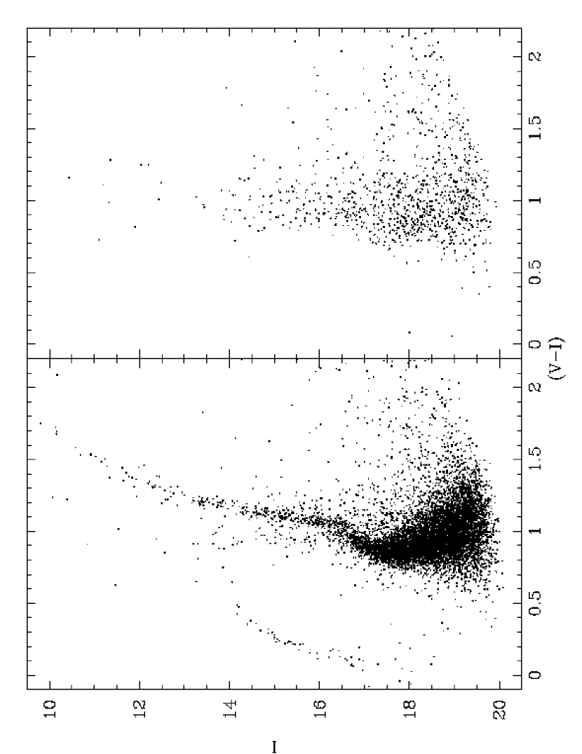
Figure 2: Left panel: Dereddened CMD for M10 stars with $3\farcm 4<r<8\farcm 5$ from the cluster center. Right panel: Dereddened CMD for stars with $r>11.\farcm 3$ from the cluster center. Most of these stars are likely to belong to the field.

We obtained $BVI$ photometry for nearly 25,000 stars reaching from the tip of the red giant branch (RGB) to over 1.5 magnitudes below the turnoff in $I$ from the KPNO images. Fig. 2 shows our $VI$ photometry for a subsample eliminating the center of the cluster (to eliminate many blended stars) and the outskirts (where field stars start to dominate) in order to illustrate the photometric quality. The photometry was corrected for differential extinction using the extinction map from von Braun et. al. (2002), which noticeably reduced the scatter around the cluster sequences in the color-magnitude diagram (CMD). We focus on the $I$-band LF in order to minimize the residual effects of the differential reddening.

We determined the cluster fiducial line from the dereddened dataset using a method similar to that of Hargis et al. (2004). Main sequence points were determined from the mode of stars in magnitude bins, while subgiant branch stars were determined from the mode of stars in color bins. On the red giant branch, fiducial points were determined from means. The fiducial is provided in Table 1.

2.2 High-Resolution Data

We reduced additional observations of the core of the cluster using the High-Resolution Camera (McClure et al., 1989) on the 3.6m Canada-France-Hawaii Telescope (CFHT) on 13 April 1993. In all, there were eleven $B$-band exposures ($1\times 60$s, $10\times 300$s) and fourteen $I$-band exposures ($2\times 6$s, $12\times 160$s). The observations used a 1200 $\times$ 1200 pixel Loral 3 CCD with 0$\farcs$11 pixel^-1 for a total field of 2$\farcm$2 $\times$ 2$\farcm$2. The images were processed similarly to the KPNO images, with the exception that only twilight flat images were employed. The High-Resolution Camera used a closed-loop, fast tip-tilt correction system to obtain very good image quality. Seeing ranged from about 0$\farcs$5 (FWHM) to 0$\farcs$9 for the M10 images.

The CFHT photometry was calibrated against KPNO photometry for 125 horizontal branch and bright giant branch stars. The transformation equations used were

$$b=B+a_{0,i}+a_{1}*(B-I)$$

$$i=I+b_{0,i}+b_{1}*(B-I)$$

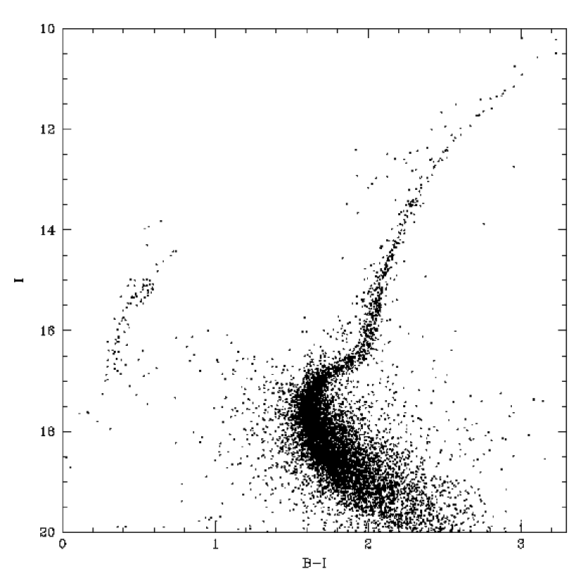
Figure 4: ($I,B-I$) color-magnitude diagram for the entire CFHT dataset.

where $a_{0,i}$ and $b_{0,i}$ are zero-point corrections determined for each CFHT image. Fig. 3 shows the residuals for the calibration. The average residuals were less than 0.01 mag in $B$, $I$, and $(B-I)$. No significant color trends were noticeable among the red giant stars, although there may be a small trend among the horizontal branch stars. Because the horizontal branch stars do not impact our luminosity function considerations, we have not pursued the issue. The final color-magnitude diagram is shown in Fig. 4.

2.3 Artificial Star Tests and Completeness Corrections

To quantify the completeness in detecting and counting stars as a function of magnitude and position in the cluster, we performed extensive artificial star tests on the KPNO images following the same procedure described by Hargis et al. (2004). One modification made for this study was the addition of appropriate differential reddening for each artificial star according to its position in the frame. Positions for the artificial stars were chosen at random within a grid such that no artificial stars overlapped [separations were no smaller than 2 $\times$ PSF radius + 1 pixel; Piotto & Zoccali (1999)]. Artificial star tests were only conducted on the $V$ and $I$ frames, with approximately 2000 stars added per frame per run. The artificial star frames were processed in a manner identical to our initial photometric reduction. In all, we conducted 56 runs involving 91757 artificial stars. The artificial star tests were used to compute median color and magnitude biases $\left[\delta_{I}\equiv\mbox{median}(I_{output}-I_{input})\right]$, median external color and magnitude error estimates $\left[\sigma_{ext}(I)\equiv\mbox{median}\mid\delta_{I}-\mbox{median}(\delta_{I})\mid/0.6745\right]$, and total recovery probabilities $\left[F(I)\right]$. These quantities are used to correct the LF for incompleteness and magnitude biases (Sandquist et al., 1996), so we must be able to find their values as a function of magnitude and position. We fitted the external magnitude errors using functional forms given in Sandquist et al. (1996). We found that linear interpolation for $\delta$ and $F$ as a function of magnitude produced an improved description of the behavior at the faint end of the sample. A relatively small number of artificial stars were placed in the innermost radial bin due to its small area, so we resorted to fits using functions from (Sandquist et al., 1996). Radial interpolation was accomplished using polynomial functions. We present the results for $\sigma_{ext}$, $\delta$, and $F$ as a function of input artificial star magnitude and radius in Figs. 5 - 7.

The completeness corrections $f$ were subsequently computed following the procedure of Sandquist et al. (1996). $f$ was set to 1 for stars brighter than the cluster turnoff to minimize numerical noise in the final LF. Fig. 8 show the results for the completeness corrections as a function of output magnitude and radius. In two of the radial bins close to the cluster core, blending causes $f$ to become substantially greater than 1. This fact drove our decision to limit the luminosity function to $I<19$ even though the photometry is nearly 100% complete for fainter stars farther from the cluster center.

2.4 Field Star Correction

A significant field star population covers the cluster field, and the field stars overlap the cluster fiducial in the CMD on the main sequence, subgiant branch, and lower giant branch. The primary source of contamination is from foreground main sequence stars in the Galactic disk. We attempted to minimize field star contamination by eliminating stars more than 9$\farcm$6 from the cluster center. We used stars more than 11$\farcm$3 from the center to determine field star corrections for the LF. As can be seen in the CMD of Fig. 2, the cluster star population is not readily apparent in the outer parts of the image. To determine the field correction, we determined the contribution to the LF from the outer portions of the field, and multiplied it by a factor of 1.97 to account for the difference in areal coverage. This correction will be an overestimate of the true field star correction because we have not accounted for the small population of cluster stars falling in the outer parts of the images.

2.5 The Luminosity Function

Using the results of the artificial star tests (particularly the completeness factor $f$), we computed the observed LF following the procedure of Sandquist et al. (1996). The LF for the KPNO data was calculated by multiplying each star detected on the object images by the factor $f^{-1}$, which was tabulated as a function of magnitude and radius. We selected stars for the LF that were less than $5\sigma_{ext}$ (color and magnitude distance) from the fiducial line determined for the cluster (Fig. 9). Because of the effects of crowding near the cluster center in the KPNO images, we did not consider main-sequence stars within 170″of the cluster center or evolved stars within 68″. A correction was applied to the evolved star sample to account for the differences in spatial coverage (Sandquist et al., 1996).

The field-star-corrected portion of the LF is shown in Fig. 10. The corrected and uncorrected $I$-band luminosity functions are presented in Table 2. Notable corrections (relative to the size of the sample from the central regions of the cluster) were in the bins at $I=16.37$ and 16.57. The field correction here significantly changes the shape of the LF at the join between the SGB and the lower RGB. Smaller corrections are needed in brighter bins on the RGB (with the exception of one bin at $I=13.97$, which becomes consistent with 0 to within the errors when corrected). No field stars are found in the regions of the CMD populated by RGB stars in the red giant bump ($I\sim 13.5$) and brighter because the giant branch slopes away from the disk main sequence population. We will return to the subject of the field star contamination in §4.

2.5.1 The Combined Luminosity Function

We produced a “global” LF combining data from the KPNO and CFHT images in order to test the reality of features on the RGB. We have broken the LF into three magnitude ranges:

BRIGHT ($I<15.07$): For bright RGB stars, we took photometry from the CFHT images for the center of the cluster and from the KPNO images for stars with $r>68\arcsec$. Extinction differences between the CFHT field and the reference field of von Braun et al. (2002) were also accounted for. There is a small amount of area near the core that is not covered by either dataset. A small number of stars were measured in both, but were only counted once for the final LF. AGB stars can be clearly distinguished from RGB stars in both samples, so there is minimal contamination.

MIDRANGE ($15.07<I<17.67$): KPNO stars were only used if $r>170\arcsec$, and incompleteness corrections from the artificial star tests were also employed. CFHT stars were used for $r>16\farcs 5$, but no incompleteness corrections were applied.

FAINT ($I>17.67$): Only KPNO stars with $r>170$ were used and incompleteness corrections were applied.

The BRIGHT and MIDRANGE segments of the combined LF were normalized to samples with $r>170\arcsec$ using stars in the ranges $13.07<I<15.07$ and $15.07<I<16.07$, respectively.

In the lower panel of Fig. 10, we compare the field-star-corrected KPNO, CFHT, and combined LFs for the cluster. The three agree very well, indicating that there is little or no radial variation in the RGB populations. We will return to this issue in §5.

3 M10 Characteristics: Age, Metallicity, Reddening, and Distance Modulus

Before we compare the observed LF with theoretical models, we discuss the accepted ranges for cluster characteristics (age, metallicity, reddening zeropoint, and distance modulus).

The latest studies of the cosmic background radiation data from WMAP have found the age of the universe to be 13.7$\pm$0.2 Gyr (Spergel et al., 2003), setting a tight upper limit on the possible ages of GGCs. Using the relative age indicator $\Delta V^{HB}_{TO}$ (defined as the magnitude difference between the $V$ magnitude of the ZAHB and MSTO points), Rosenberg et al. (1999) (which uses the homogeneous data set presented in Rosenberg et al. (2000)) found a value of $\Delta V^{HB}_{TO}$ = 3.50$\pm$0.11 for M10. The $\Delta V^{HB}_{TO}$ value indicates that M10 is coeval with the oldest globular clusters (to within the measurement errors), so that we will only consider absolute ages between 11 and 13 Gyr. Theoretical models that include helium diffusion (Kim et al., 2002) adequately model the cluster CMD with this constraint, but we have also compared the observed LF with models (Bergbusch & VandenBerg, 2001) that do not include helium diffusion and which require us to assume that the cluster is older than this range of ages.

There have been a number of determinations of [Fe/H] for M10, and published values range over about 0.4 dex. The two most widely used metallicity scales are those of Zinn & West (1984) and Carretta & Gratton (1997), and we considered both in our comparisons. Zinn & West (ZW) cite a value of [Fe/H] = $-1.60$. Using high-resolution spectra of GGC red giants, Carretta & Gratton (CG) measured [Fe/H] $=-1.41\pm 0.02$. Systematic differences between the two scales are well-documented, with the CG scale giving a higher metallicity by approximately $0.2-0.3$ dex for low- or intermediate-metallicity clusters. Spectroscopic measurements of the infrared Ca II triplet of M10 red giants have also been made by Rutledge et al. (1997). Rutledge, Hesser, & Stetson (1997) used these measurements to compute abundances on the ZW and CG scales of [Fe/H]${}_{ZW}=-1.55\pm 0.04$ and [Fe/H]${}_{CG}=-1.25\pm 0.03$. Recent high-resolution spectra taken by Kraft & Ivans (2003) were also used to measure a metallicity [Fe/H]_KI between $-1.41$ and $-1.48$ (dependent on the model atmospheres used in the analysis).

In this study, we adopt the reddening values determined by von Braun et al. (2002). We note, however, that their mean reddening value of E$(V-I)$ = 0.28 disagrees with the value E$(V-I)$ = 0.39 derived from COBE infrared dust emissivity maps by Schlegel, Finkbeiner, & Davis (1998). Although we do not directly use the mean E$(V-I)$ value, the reddening issue is a significant source of systematic uncertainty in doing absolute comparisons with theoretical LFs, and so it is further discussed below.

We computed the distance modulus via subdwarf fitting to the main sequence photometry of von Braun et al. (2002) because our photometry did not reach faint enough on the MS to be useful for this purpose. We used $Hipparcos$ parallaxes and subdwarf metallicities from Carretta et al. (2000) as discussed in Hargis et al. (2004). Relative to von Braun’s differentially dereddened data, $(m-M)_{V}=14.18\pm 0.04$ for our “best” assumptions: the reddening zero point E$(V-I)$ = 0.23 (von Braun et al., 2002), and [Fe/H]=$-1.41$ from Carretta & Gratton (1997). (Note that the reddening zero point is not the same as the average reddening. The reddening zero point is the average reddening of a $280\arcsec\times 280\arcsec$ subfield chosen as a reference by von Braun et al. for their larger M10 field.) By far the uncertainty in the reddening zero point is going to be the largest systematic error. A 0.01 mag error in E$(V-I)$ gives roughly a 0.054 mag error in the distance modulus. Unfortunately the systematic error in the zero point cannot be determined well. Reddening maps from COBE data (Schlegel, Finkbeiner, & Davis, 1998) indicate E$(V-I)$ = 0.34 for the reddening zero point. The COBE zero point can effectively be ruled out given that i) it implies a distance modulus of 14.72, ii) M10 and M12 appear to be coeval with nearly identical metallicities, and iii) the difference between the distance moduli of M10 and M12 is no more than about 0.2 mag based on the CMD. As evidence of this we present the fiducial lines of the two clusters in Fig.11. The data from the two clusters were taken during the same observing run, and calibrated nearly identically.

However, based on the COBE results, it is more likely that the reddening zero point is larger than that of von Braun et al. (2002) rather than smaller. Thus we consider a distance modulus range $(m-M)_{V}=14.18^{+0.15}_{-0.06}$ set by our estimation of the systematic reddening uncertainties. When incorporating the systematic difference between von Braun’s data and ours (his is fainter than ours by 0.08 mag on average), this gives $(m-M)_{V}=14.10^{+0.15}_{-0.06}$, which is consistent with the distance estimates from Ferraro et al. (1999) using the horizontal branch. Using the Ferraro et al. value of E$(B-V)=0.28$ and $A_{V}/{E(B-V)}=3.1$, we calculate values of $(m-M)_{V}^{CG97}=14.25$ and $(m-M)_{V}^{[M/H]}=14.22$ from their tables. By way of comparison, the distance modulus for M12 derived via an almost identical procedure was $(m-M)_{V}^{M12}=14.05\pm 0.12$ (assuming [Fe/H]${}_{M12}=-1.41$ and E$(V-I)_{M12}=0.25\pm 0.02$).

4 The Luminosity Function

4.1 Comparison with Models

In Fig. 12, we compare the observed luminosity function of M10 with theoretical models covering realistic ranges in [Fe/H] and distance modulus, and with different sets of models from Kim et al. (2002) and Bergbusch & VandenBerg (2001). The models are normalized on the main sequence below the turnoff (at $I\sim 18.5$), with the mass function exponent $x=2$ chosen to match the slope of the main sequence LF. Models with varying age are not plotted because within the acceptable age range there is little difference in the degree of agreement between models and observations. For realistic choices of age, [Fe/H], and distance modulus, we find that the number of stars on the lower RGB relative to main sequence stars is in good agreement with models. The RGB bump is detected at $I\sim 13.3$.

There are a couple of deviations from the theoretical models that deserve additional discussion. There is a significant secondary bump at $14<I<15$. There is an increase in counts in this range for both the KPNO and CFHT datasets individually, and field star corrections do not remove the feature. There also seems to be a significant excess in counts brighter than the RGB bump in the range $12.2<I<13.2$. In Fig. 12, this excess is masked somewhat by the theoretical predictions for the RGB bump. (We will not discuss the RGB bump in detail, however.) On a final note, the main sequence mass function exponent ($x\approx 2$) is relatively large as well, in agreement with the results of Piotto & Zoccali (1999).

To gauge the significance of the apparent excesses of RGB stars relative to main sequence stars in Fig. 12, we devised a ratio of the number of stars in a magnitude range on the RGB to the number near the cluster turnoff. This selection is based on the finding of Stetson (1991) that cluster luminosity functions very nearly overlie one another (independent of [Fe/H], [$\alpha$/Fe], age, and initial mass function; see also VandenBerg, Larson, & de Propris (1998)) when they are shifted so that the turnoffs are coincident in magnitude. By defining samples of cluster stars relative to easily-measured points on the cluster’s fiducial line and taking the ratio of samples, we can nearly eliminate uncertainties resulting from imperfectly known cluster parameters and from the shifting and normalization of the theoretical luminosity functions. In addition, statistical errors are easy to determine using Poisson statistics.

We define the magnitude range of the RGB sample ($N_{RGB}$) relative to the turnoff magnitude $I_{TO}$ ($17.52\pm 0.10$ for M10). The turnoff sample $N_{TO}$ is selected from the stars in a 0.4-magnitude wide bin centered on $I_{MSTO}$. Because our final luminosity function employs corrections for field contamination and incompleteness, we computed the ratio from the LF. For the count excess in $14<I<15$, we find a ratio $N_{RGB}/N_{TO}=0.116\pm 0.006$, and for the excess with $12.2<I<13.2$, $N_{RGB}/N_{TO}=0.0354\pm 0.002$. The major source of systematic uncertainty is the measurement of $I_{TO}$; if it shifts with respect to the RGB magnitude range being used, the ratio value changes substantially. If $I_{TO}=17.42$, the two ratios become 0.130 and 0.0397, and they become 0.103 and 0.0312 if $I_{TO}=17.62$.

Using theoretical models, we can compute expected values for the ratios. From the Yonsei-Yale isochrones (Kim et al., 2002), we find ratios of 0.0694 and 0.0227 for [Fe/H]$=-1.41$, [$\alpha$/Fe] = 0.3, age 12 Gyr, and mass function exponent $x=2.0$. Because our reference population is at the turnoff and not fainter, the ratios are insensitive to large changes in the mass function exponent. Reducing the mass function exponent to $x=-0.5$ only increases the ratios to 0.0771 and 0.0254, respectively — stellar evolution, rather than star formation processes, dominates the ratio. Between the ages of 10.5 and 13.5 Gyr, the theoretical predictions for $N_{RGB}/N_{MSTO}$ change by only 0.0095 and 0.0056, respectively. Over the metallicity range $-1.61\leq\mbox{[Fe/H]}\leq-1.41$, the theoretical predictions for the two ratios change by only 0.0089 and 0.0013, respectively. Thus, no reasonable variation of parameters like age or [Fe/H] or possible errors in the determination of $I_{MSTO}$ is able to account for the excess of RGB stars in the observed LF of M10. Comparing our best observational value and the best theoretical model, the differences are significant at more than the $7\sigma$ and $6\sigma$ levels for the samples fainter than ($14<I<15$) and brighter than ($12.2<I<13.2$) the RGB bump.

4.2 Comparison with M12

In addition to comparing the LF to theoretical models, it is also valuable to compare to other globular clusters. The cluster M12 provides an excellent comparison. Using relative age indicators, we find that the ages of M10 and M12 are consistent to within measurement errors. The color differences between the turnoff and red giant branch (see Fig. 11) and the magnitude differences between turnoff and horizontal branch ($\Delta V^{HB}_{TO}=3.60\pm 0.12$ for M12) are both close for the two clusters. The metallicities are also close: the ZW values only differ by 0.01 dex, while Rutledge, Hesser, & Stetson (1997) measurements indicate a difference of 0.15 dex or less with M12 the more metal-rich (consistent with its redder upper RGB). The distances of the two clusters are also the same to within the measurement errors. One notable difference between the clusters is the main sequence mass function exponent $x$: Hargis et al. (2004) found $x=0$ for M12, while we find $x=2$ for M10 in this study.

The differences in mass function mean that the two LFs cannot be compared simply by correcting for differences in distance modulus and normalizing them using main sequence stars. When the star counts for the two clusters are normalized near the turnoff, there are more M10 stars than M12 stars in the magnitude ranges discussed above. We can quantify this using the same RGB-MS ratio for the cluster M12 using data from Hargis et al. (2004) since the “best” model parameters are nearly identical between the two clusters. Hargis et al. found that the M12 LF showed no excess of RGB stars compared to theory when the LF is normalized to the main sequence. So, as expected we find $N_{RGB}/N_{MSTO}=0.083\pm 0.008$ for the faint sample in M12 ($13.95<I<14.95$) as compared to 0.0755 from Y² models (for [Fe/H] = -1.41, age 12 Gyr, and mass function exponent $x=0$) and $0.116\pm 0.006$ for M10. For the brighter sample ($12.15<I<13.15$), the ratio is $0.021\pm 0.002$ for M12, compared to 0.025 from Y² models and 0.0354 for M10. So, the population ratio values for M12 agree with theoretical predictions to less than 1 and $2\sigma$, while the corresponding ratios for M10 differ by more than 7 and $6\sigma$, respectively. Thus, M10 has an excess of RGB stars relative to MS stars when compared to another well-studied, nearly-identical cluster.

5 Discussion

Both the comparison between M10 and theoretical predictions and between M10 and the nearly identical cluster M12 indicate that the LF of M10 is anomalous. The RGB-MS ratio defined above is insensitive to the parameters age and heavy element content ([Fe/H] and [$\alpha$/Fe] particularly), which allows us to eliminate them from consideration as the cause. In addition to having an age and heavy element content that is identical to that of M10 to within current observational errors, M12 has a CMD morphology (most notably a blue horizontal branch tail) that is very nearly the same as M10. Whatever the cause of M10’s unusual LF, it does not seem to create noticeable differences in the evolutionary tracks of stars in the CMD except possibly near the RGB tip (see Fig. 11).

Field-star contamination (or errors involved in correcting for this contamination) are unlikely to explain the unusual features of the LF. Field stars are easily visible in the CMD brighter than the subgiant branch, and can also be detected fainter than the turnoff based on their colors (significantly redder than the cluster fiducial, even when the data is dereddened) and based on their lack of any concentration toward the cluster center (see Fig. 2). Once corrected, the LF of the main sequence, subgiant branch, and part of the lower red giant branch agrees very well with theoretical predictions (see Fig. 10). However, field star contamination is not strong enough to explain the LF excess just below the RGB bump, and contamination is negligible above the bump since the field star distribution clearly diverges from the RGB for $I\lesssim 15.5$. In addition, because the excess star counts are measured in both the core and envelope of the cluster, we can rule out most other sorts of foreground or background contamination.

It is natural to expect that unusual features in LFs should result from physics that affects the evolutionary timescales of the stars. If that is the case here, we should look at factors that affect the rate at which nuclear fuel is processed. The abundance of helium and CNO elements enter into the determination of the instantaneous nuclear reaction rate at any point in a star, yet theoretical models indicate that the abundance of CNO elements does not significantly affect the relative numbers of RGB and MS stars while helium abundance plays a more substantial role (Stetson, 1991; VandenBerg, Larson, & de Propris, 1998). The reason for this can be seen in the study of Ratcliff (1987) — the evolutionary timescale for red giants is not changed by variations in helium abundance, but the MS timescale is. We believe that this can be understood qualitatively as being due to the nature of the structure of red giants: the rate of nuclear reactions in the hydrogen fusion shell is set entirely by the star’s need to support the envelope and the position of the shell source (set by the size of the degenerate core). The structural constraints on giant stars are responsible for the luminosity – core mass relations found in theoretical models of giant stars. When put in this framework, the possible causes of the discrepancy seen in M10 are more easily seen.

The evolutionary timescale for red giants can be modified (independently of the MS) if there is a change in the way the envelope of the giant is supported. An example of this is seen in the rotating models of VandenBerg, Larson, & de Propris (1998) in which angular momentum was assumed to be conserved in radiative shells and convection zones were assumed to rotate like solid bodies. In the red giant stage, the contraction of the core leads to rapid rotation that provides a modest amount of centrifugal support to the star’s envelope. This relieves the fusion shell of some of the burden of supporting the envelope (or in other words, the density of the fusion shell decreases somewhat, causing a decrease in the energy output of the shell). The degree of centrifugal support changes as the star evolves thanks to continued contraction of the core as additional mass is added by the fusion shell. Indirect evidence for significant core rotation comes from cluster horizontal branch stars (e.g. Behr 2003): rotational velocities for some of these stars can reach as high as 40 km s^-1. Although this is intriguing, we are far from completely understanding the angular momentum evolution of giant stars, and there is no reason to believe that M10 stars have unusually high rotation on average. In addition, the relatively good agreement of observations and theory on the lower red giant branch argues against a process that modifies the evolutionary timescales from the beginning of the red giant branch.

For related reasons, we predict that so-called “deep mixing” on the RGB should not have a significant long-term effect on the evolutionary timescales of giant stars unless the extra mixing is somehow related to an alternate means of envelope support. (“Deep mixing” processes are known to produce O-Na anticorrelations at the surfaces of bright giants in many clusters.) Changes to the chemical makeup of the material being processed by the fusion shell causes the shell and envelope of the star to adjust on a timescale much shorter than the lifetime of the red giant phase. The best-known example of this is the red giant bump. When the fusion shell reaches what was the base of the envelope convection zone (in which the gas has a higher hydrogen content), the star’s evolution temporarily slows as it adjusts to the new fuel mix. However, the slope of the differential LF function after the bump is not significantly different from what it was before, which means that the evolutionary timescales of the RGB stars are once again enforced by the structure. So, while there could be modifications to the cluster LF if deep mixing begins at a position different than the red giant bump, extended periods of deep mixing would not change the evolutionary timescale once the star’s envelope has adjusted. Spectroscopic analysis of M10 giants (Kraft et al., 1995) add some credence to this idea since M10 giants on average have oxygen depletions between that of M3 (a cluster that has a theoretically-predicted ratio of giants to main sequence stars (Rood et al., 1999)) and M13. So unless the adjustment timescale for the stellar envelope (approximately the Kelvin-Helmholtz timescale) is several times longer than that predicted for RGB bump stars evolving via standard physics and the star’s brightness varies by several magnitudes during this time, it would be difficult to explain M10’s LF in this way.

Ratios of giants to main sequence stars are obviously a function of the evolutionary timescales of both main sequence stars and giants. For MS stars, differences in initial helium abundance cause related differences in evolutionary timescale for the simple reason that the amount of fuel changes (although there are additional effects resulting from changes to the star’s luminosity). We do not believe that differences in initial helium content are to blame because i) a large positive enhancement would be necessary for M10, bringing M10’s helium content close to the solar value and going against expected nucleosynthetic trends ($\Delta Y/\Delta Z>0$) (VandenBerg, Larson, & de Propris, 1998), ii) evidence from the helium abundance indicator $R$ shows that the globular cluster system as a whole does not have an intrinsic spread in $Y$ of greater than 0.019 (Salaris et al., 2004), iii) there is virtually no difference in the CMD morphologies of M10 and M12, and iv) a change in main sequence timescales alone would tend to make the RGB star counts higher than predicted at all luminosity levels.

The overall insensitivity of the ratio $N_{RGB}/N_{MS}$ to most parameters that vary from cluster to cluster makes M10’s LF difficult to understand. The theoretical results do help to emphasize that in spite of the substantial structural differences between MS and RGB stars, there is a very strong connection between their evolutionary timescales. However, we must also keep in mind that clusters are made of individual stars. From the time a star reaches the turnoff of a globular cluster, it can take approximately 2 Gyr to reach the middle of the RGB (Yi, Kim, & Demarque, 2003). While the mass function of current main sequence stars can be estimated from the slope of the LF, the mass function of now-evolved stars cannot — in fact, it may be different. Typically, theoretical LFs assume that the slope of the initial mass function for stars in a cluster is a constant. If this is not the case, then $N_{RGB}/N_{MS}$ could differ from its well-determined theoretical value.

The question remains whether such a variation in the initial mass function could be due to a statistical fluctuation or whether it would have to result from a stronger trend in the mass function of cluster stars. For $12.2<I<13.2$, 79 stars were identified while only about 51 were expected. For $14<I<15$, 250 stars were identified, and 149 were expected theoretically. Poisson fluctuations ($\sqrt{N}$) in “normal” samples of stars as a function of mass therefore seem unlikely to account for the M10 observations. All of the stars currently on the giant branch would have originated from just one LF bin at the turnoff approximately 2 Gyr ago, but even Poisson fluctuations in a sample that size ($<1000$ stars) are several times too small to explain the giant branch excesses we see.

Another possibility is that the mass function at the cluster turnoff about 2 Gyr ago deviated more systematically from the power-law form assumed in models. Although this hypothesis cannot be tested directly, we can look for signs of significant variations in mass function slope on the current main sequence. We compared the bin-to-bin LF slopes with theoretical values using the best “average” mass function exponent $x=2.0$. On the upper main sequence, several bins near the turnoff deviate from the theoretical LF slopes by between 2 and $3\sigma$, and one interval ($18.57<I<18.77$) closer to our faint limit deviates by almost $4.3\sigma$.

Of the main sequence LFs for M10, M22, and M55 discussed by Piotto & Zoccali (1999), M10’s LF was least consistent with having a constant mass function slope $x$ (although there is significant uncertainty in the mass-luminosity relation for the low mass stars). We note once again that an examination of the LF (Piotto & Zoccali, 1999) indicates that there is a noticeable drop in the main sequence luminosity function for $21\lesssim V\lesssim 23$ (it is less obvious in $I$), so that it is not unreasonable to believe that there might have been another mass function variation among stars that have now left the main sequence. The anomaly seen in our LF of the evolved stars of M10 implies that there may have been a greater number of MS stars than expected from the $x=2$ mass function derived from the upper main sequence LF.

A simple understanding of dynamical processes (like evaporation) would lead us to expect that strong dynamical effects would tend to remove low mass stars from a cluster, making the mass function shallower. Because the main sequence LF observed by Piotto & Zoccali (1999) is much steeper than those of M22 and M55 (but comparable to the metal-poorer clusters M15, M30, and M92), the implication is that M10 has been affected in a comparatively minor way. Even if dynamics are responsible for modifying M10’s LF, we are again left to explain why M12 does not show a similar effect, given that the characteristics of its Galactic orbit are similar to that of M10 (Dinescu, Girard, & van Altena, 1999).

In the end, we do not have a satisfying explanation for the unusual aspects of M10’s LF, but the cause can be external to the stars themselves. Though there is evidence for mass function variations (changes in mass function slope) from other parts of M10’s LF, we still have no explanation for why they might be present in a massive cluster like M10. Although the hypothesis is difficult to test, there are two possible avenues to follow. First, continued searches for unusual RGB luminosity functions in other globular clusters may turn up additional examples that would help to identify a relationship to cluster parameters (although the most obvious correlations with metallicity or horizontal branch morphology seem to be ruled out by previously published LFs) or identify whether RGB anomalies cover similar or different ranges of luminosity. Second, main sequence luminosity functions using larger samples would help answer the question of whether significant (non-Poissonian) LF fluctuations exist within clusters. Most deep MS LFs have been derived using the WFPC2 imager on the Hubble Space Telescope. Wide-field high spatial-resolution instruments (like the Advanced Camera for Surveys on HST or cameras on the CFHT) would be ideal for surveying the larger areas necessary.

Figure 1: Residuals (in the sense of ours minus theirs) from 13,000 stars in common with von Braun et al. (2002).

Figure 3: Residuals (in the sense of CFHT minus KPNO) from 125 stars used to calibrate the CFHT data.

Figure 5: Results from the artificial star tests for the external $I$ magnitude errors $\sigma_{ext}(I)$ as a function of radius and input magnitude.

Figure 6: Results from the artificial star tests for the $I$ magnitude biases $\delta(I)$ as a function of radius and input magnitude.

Figure 7: Results from the artificial star tests for the total recovery probability $F$ as a function of radius and input magnitude.

Figure 8: Results from the artificial star tests for the completeness fraction $f$ as a function of radius and output magnitude.

Figure 9: Left panel: Dereddened CMD for measured M10 stars with $r<2\farcm 3$ from the cluster center. Middle and right panels: Stars that were and were not selected for the LF above the faint limit ($I=19.2$).

Figure 10: Upper panel: The $I$-band luminosity function with corrections and without corrections for field star contamination. No field stars were detected for $I<13.9$. Lower panel: Comparison of luminosity functions for the KPNO, CFHT, and combined star samples.

Figure 11: Comparison of the fiducial lines of the clusters M10 (open circles) and M12 (solid circles). The turnoff colors of the fiducials were nearly identical in color, so that the fiducials were rectified by shifting in magnitude (M10 was 0.107 mag fainter) so that the points on the main sequence 0.05 mag redder than the turnoff were aligned.

Figure 12: Comparisons between the observed LF (combined sample) of M10 and theoretical models. Top panel: models with varying [Fe/H]. Middle panel: models with varying distance modulus. Bottom panel: models with “best” choices for [Fe/H], distance modulus, and ages from Bergbusch & VandenBerg (2001) and Kim et al. (2002).

Table 1: M10 $(I,V-I)$ Fiducial Points

$I$	$V-I$	$N$
19.4000	1.0327	1072
19.2000	1.0109	1353
19.0000	0.9778	1531
18.8000	0.9642	1536
18.6000	0.9203	1470
18.4000	0.9168	1427
18.2000	0.8994	1391
18.0000	0.8837	1329
17.8000	0.8710	1140
17.6000	0.8594	1067

Note. — The complete version of this table is in the electronic edition of the Journal. The printed edition contains only a sample.

Table 2: M10 $I$-band Luminosity Function

$I$	$N$	$\sigma_{N}$	$N$	$\sigma_{N}$	$N$	$N$	$\sigma_{N}$
	KPNO Uncorrected		Field Star Corrected		CFHT	Combined
9.77	0.517	0.517	0.517	0.517	0	0.342	0.342
10.17	2.067	1.033	2.067	1.033	1	1.709	0.764
10.37	0.000		0.000		1	0.342	0.342
10.57	1.033	0.731	1.033	0.731	2	1.367	0.683
10.77	1.550	0.895	1.550	0.895	1	1.025	0.592
10.97	2.067	1.033	2.067	1.033	0	1.367	0.683
11.17	2.583	1.155	2.583	1.155	5	3.417	1.081
11.37	1.550	0.895	1.550	0.895	1	1.367	0.683
11.57	3.617	1.367	3.617	1.367	5	3.417	1.081
11.77	3.100	1.266	3.100	1.266	1	2.050	0.837
11.97	4.651	1.550	4.651	1.550	3	4.101	1.184

Note. — The complete version of this table is in the electronic edition of the Journal. The printed edition contains only a sample.

References

- Behr (2003) Behr, B. B. 2003, ApJS, 149, 67
- Bergbusch (1996) Bergbusch, P. A. 1996, AJ, 112, 1061
- Bergbusch & VandenBerg (2001) Bergbusch, P. A., & VandenBerg, D. A. 2001, ApJ, 556, 322
- Bolte (1994) Bolte, M. 1994, ApJ, 431, 223
- Carretta & Gratton (1997) Carretta, E. & Gratton, R. G. 1997, A&AS, 121, 95
- Carretta et al. (2000) Carretta, E., Gratton, R. G., Clementini, G., & Fusi Pecci, F. 2000, ApJ, 533, 215
- Cohen et al. (1997) Cohen, R. L., Guhathakurta, P., Yanny, B., Schneider, D. P., & Bahcall, J. N. 1997, AJ, 113, 669
- Dinescu, Girard, & van Altena (1999) Dinescu, D. I., Girard, T. M., & van Altena, W. F. 1999, AJ, 117, 1792
- Ferraro et al. (1999) Ferraro, F.R., Messineo, M., Fusi Pecci, F., de Palo, M.A., Straniero, O., Chieffi, A., & Limongi, M. 1999, AJ, 118, 1738
- Guhathakurta et al. (1998) Guhathakurta, P., Webster, Z. T., Yanny, B., Schneider, D. P., & Bahcall, J. N. 1998, AJ, 116, 1757
- Hargis et al. (2004) Hargis, J.R., Sandquist, E.L., & Bolte, M. 2004, ApJ, 608, 243
- Hurley, Richer, & Fahlman (1989) Hurley, D. J. C., Richer, H. B., & Fahlman, G. G. 1989, AJ, 98, 2124
- Kim et al. (2002) Kim, Y., Demarque, P., Yi, S. K., & Alexander, D. R. 2002, ApJS, 143, 499
- Kraft et al. (1995) Kraft, R. P., Sneden, C., Langer, G. E., Shetrone, M. D., & Bolte, M. 1995, AJ, 109, 2586
- Kraft & Ivans (2003) Kraft, R. P. & Ivans, I. I. 2003, PASP, 115, 143
- McClure et al. (1989) McClure, R. D., Grundmann, W. A., Rambold, W. N., Fletcher, J. M., Richardson, E. H., Stillburn, J. R., Racine, R., Christian, C. A. & Waddell, P. 1989, PASP, 101, 1156
- Piotto & Zoccali (1999) Piotto, G. & Zoccali, M. 1999, A&A, 345, 485
- Ratcliff (1987) Ratcliff, S. J. 1987, ApJ, 318, 196
- Renzini & Fusi Pecci (1988) Renzini, A. & Fusi Pecci, F. 1988, ARA&A, 26, 199
- Rood et al. (1999) Rood, R. T., et al. 1999, ApJ, 523, 752
- Rosenberg et al. (1999) Rosenberg, A., Saviane, I., Piotto, G., & Aparicio, A. 1999, AJ, 118, 2306
- Rosenberg et al. (2000) Rosenberg, A., Aparicio, A., Saviane, I., & Piotto, G. 2000, A&AS, 145, 451
- Rutledge, Hesser, & Stetson (1997) Rutledge, G. A., Hesser, J. E., & Stetson, P. B. 1997, PASP, 109, 907
- Rutledge et al. (1997) Rutledge, G. A., Hesser, J. E., Stetson, P. B., Mateo, M., Simard, L., Bolte, M., Friel, E. D., & Copin, Y. 1997, PASP, 109, 883
- Salaris et al. (2004) Salaris, M., Riello, M., Cassisi, S., & Piotto, G. 2004, A&A, 420, 911
- Sandquist et al. (1996) Sandquist, E. L., Bolte, M., Stetson, P. B., & Hesser, J. E. 1996, ApJ, 470, 910
- Sandquist et al. (1999) Sandquist, E. L., Bolte, M., Langer, G. E., Hesser, J. E., & Mendes de Oliveira, C. 1999, ApJ, 518, 262
- Schlegel, Finkbeiner, & Davis (1998) Schlegel, D. J., Finkbeiner, D. P., & Davis, M. 1998, ApJ, 500, 525
- Spergel et al. (2003) Spergel, D. N., et al. 2003, ApJS, 148, 175
- Stetson (1991) Stetson, P. B. 1991, ASP Conf. Ser. 13: The Formation and Evolution of Star Clusters, 88
- VandenBerg, Larson, & de Propris (1998) VandenBerg, D. A., Larson, A. M., & de Propris, R. 1998, PASP, 110, 98
- von Braun et al. (2002) von Braun, K., Mateo, M., Chiboucas, K., Athey, A., & Hurley-Keller, D. 2002, AJ, 124, 2067
- Yi, Kim, & Demarque (2003) Yi, S. K., Kim, Y., & Demarque, P. 2003, ApJS, 144, 259
- Zinn & West (1984) Zinn, R. & West, M. J. 1984, ApJS, 55, 45