A Catalog of Distant Compact Groups Using DPOSS

Abstract

In this paper we present an objectively defined catalog of 459 small, high density groups of galaxies out to $z\sim 0.2$ in a region of $\sim 6260$ square degrees in the northern sky derived from the Digitized Second Palomar Observatory Sky Survey. Our catalog extends down to $r=19.0$ and has a median redshift of $z_{\rm med}$ = 0.12, making it complementary to Hickson’s catalog for the nearby universe ($z_{\rm med}$ = 0.03). The depth and angular coverage of this catalog makes it valuable for studies of the general characteristics of small groups of galaxies and how galaxies evolve in and around them. We also examine the relationship between compact groups and large scale structure.

1 Introduction

Compact groups of galaxies (CGs), as the name suggests, are systems composed of a small number of galaxies in an angularly compact configuration on the sky. Stephan’s quintet is the earliest known member of this class, discovered in 1877 by Edouard Stephan. In 1948, the Seyfert sextet was found to belong to the same family. Through the nineteen-seventies, only visual detections of these systems were possible and no homogeneous sample was available for systematic studies of these low-mass structures. For a brief history of the heterogeneous samples of small groups see Iovino et al. (2003).

Rose (1977) was the first to attempt construction of an objective sample of CGs in the northern sky. By imposing a minimum requirement of three galaxies brighter than magnitude 17.5 in B-band with a density contrast of at least 1000, Rose found 170 triplets, 33 quartets, and 2 quintets over an area of $\sim$3100 degrees in the northern hemisphere. However, the most studied sample of CGs is that defined by Hickson (1982). Instead of using a fixed limiting magnitude, Hickson required that four or more galaxies have a maximum magnitude difference of 3.0 mag. The group’s surface brightness was defined as $\mu_{\rm gr}=-2.5~{}{\rm log}((\Sigma~{}10^{-0.4m_{\rm i}})/\pi\rm R_{\rm gr}^{2})$, where the $m_{\rm i}$’s are the magnitudes of the galaxies defining the group. He required a limiting surface brightness of 26.0 mag arcsec^-2 in the E-band (similar to Johnson R). He also imposed an encircling null ring where no galaxies are present of area equal to 8$\pi{\rm R_{\rm G}}^{2}$, where ${\rm R}_{\rm G}$ is the radius of the smallest circle encompassing the centers of the group members. With these constraints, Hickson found 100 CGs, covering $\sim$27000 square degrees on the sky, mostly in the north with a small extension to the south. Many studies have been performed using the Hickson sample (see Hickson 1997 for a review). From the spectroscopic survey presented in Hickson et al. (1992), out of the 100 CGs, only 69 were found to have four or more concordant galaxies, while 23 were triplets, with a median redshift $z_{\rm med}$ of 0.03 for these 92 galactic systems.

Several studies were conducted with the goal of understanding the physical nature of the CGs defined in the Hickson sample, which, despite being affected by incompleteness and bias (Prandoni et al. 1994), is comprised of interesting systems. An important question is whether or not these systems represent real dynamical structures (Hickson 1997). A critical point is that every sample selected based on an apparent density contrast will suffer from projection effects, such as a tendency to select prolate groups radially oriented along the line of sight (Plionis, Basilakos, & Tovmassian 2004), or even transient configurations (Rose 1979).

N-body simulations show that CGs might form a single giant elliptical over a few crossing times through mergers (e.g. Barnes 1985, 1989; Mamon 1987; Zheng, Valtonen, & Chernin 1993). However, CGs are observed in the local universe, which must be reconciled with these simulations. Diaferio et al. (1994) addressed this issue through a set of N-body simulations where the initial conditions emulated the properties of sparse groups. They find that although the CG lifetime seems to be short ($\sim$ 1 Gyr), the system can be constantly replenished by neighboring galaxies. These simulations succeeded in recovering observed properties of CGs including the morphological distribution with respect to the field population, the dynamical properties, and above all showed that most of the group members are not the result of mergers. A criticism of this scenario (e.g. Athanassoula 2000) is the absence of possible fossils in the field population, since in the Diaferio et al. (1994) model after a considerable fraction of the Hubble time the more massive sparse groups become an isolated giant elliptical. This problem could be alleviated by the discovery of the so-called fossil groups (Ponman et al. 1994 and Jones et al. 2003) left behind after a group merges: an elliptical embedded in an overluminous X-ray halo. A significant fraction of the group mass may also reside in a common halo outside the galaxies (see Zabludoff and Mulchaey 1998), therefore significantly slowing the rate at which the group members interact and eventually merge (see Governato et al. 1991).

The question is then how we distinguish between an elliptical originating in the field and one resulting from the merger of a sparse group. Recently, de la Rosa, de Carvalho, & Zepf (2001a), by studying the fundamental plane of elliptical galaxies in the field and in CGs, concluded that both families are similar from the structural and dynamical points of view. Proctor et al. (2004) and de la Rosa et al. (2001b), on the other hand, found that ellipticals in CGs are more similar to those in clusters than the ones in the field, based on analysis of their stellar population properties. de Carvalho et al. (1997) and Ribeiro et al. (1998), studying the vicinity of 17 CGs from the Hickson sample, out to $\sim$9000 km s^-1, found that CGs can be divided into three categories: 1) sparse groups; 2) systems with a core and a halo; and 3) real compact groups. They find that each category has its own characteristic surface density profile, which reinforces the view that CGs compose a very heterogeneous family and not a single type of system. This result not only supports the scenario envisaged by Diaferio et al. (1994) but also prompted us to investigate how CGs are distributed relative to large scale structure, including loose groups and poor and rich clusters.

Several studies examined the relation between CGs and other structures. Rood & Struble (1994) looked for structures within 1.0 Mpc (transverse) of the CGs, with a difference in radial velocity at most four times the group’s velocity dispersion. They find that 75% of Hickson’s groups are near other structures such as loose groups and Abell clusters, which might indicate that CGs are effectively part of the same hierarchy we observe in the universe, from isolated galaxies to superclusters. Similar work was done by Kelm & Focardi (2004) based on the Updated Zwicky Catalog. They generate a catalog of CGs which is quite distinct from that of Hickson, using redshifts to define galaxy aggregates. They studied the morphological characteristics of the galaxies in the vicinity of the groups using a region between 0.2 $h^{-1}$ Mpc and 1.0 $h^{-1}$ Mpc from the group center, and requiring a velocity difference less than 1000 km s^-1. These neighbor galaxies exhibit an intermediate nature between field and group galaxies, reinforcing the finding that CGs are a distinct physical entity and not merely the result of projection effects. Moreover, excluding the brightest group galaxies from the comparison, the difference in morphology distribution disappears, indicating that the group galaxy population is more evolved than field galaxies. Helsdon & Ponman (2000a,b) offer a different perspective by combining CGs and loose groups into a single sample and examining their X-ray properties. They suggest that both clustering scales should be considered together since their X-ray properties are very similar.

Although the importance of CGs in linking AGN and environment may appear obvious, only recently has the level of nuclear activity (AGN) and starburst activity among compact group galaxies been systematically measured (Coziol et al. 1998a, 1998b). Based on an analysis of 82 bright galaxies from 17 CGs, these authors found that AGN are mainly located in early-type and luminous systems, which are similar to their hosts in the field (Phillips et al. 1986). Coziol et al. (1998a) also found that AGN are more concentrated towards the central parts of the groups, suggesting a morphology-density-activity relation. This finding was later confirmed by Coziol, Iovino, & de Carvalho (2000) studying a sample of CGs defined by Iovino (2002). This may prove to be an important diagnostic of how dynamically evolved a CG is. Several other works examined the question of how the environment is related to the physical mechanism responsible for the feeding of galactic nuclei (Shimada et al. 2000, Schmitt 2001, Coziol et al. 2004, Kelm, Focardi, & Zitelli 2004).

Recently, two large samples of CGs were published. The first was selected from the Digitized Second Palomar Observatory Sky Survey (DPOSS) and based on plate data (Iovino et al. 2003), while the second by Lee et al. (2004) used the Sloan Digital Sky Survey (SDSS) and was based on CCD data. When comparing both samples it is important to consider the methodology employed to define a small group of galaxies, which is always a difficult task. The main advantage of both contributions over all previous works is the objective nature of the algorithms used to select the systems, making comparisons with models and between the surveys more meaningful. A similar approach was used for the first time in Prandoni et al. (1994), and Iovino (2002) also defines a sample of CGs in a totally automated fashion.

Compact groups are thought to be ideal places to study galaxy evolution, since their high density and low velocity dispersion naively imply a higher merging rate. The observational evidence from nearby CGs shows that this is not necessarily true in a majority of cases. Thus, better understanding of the weaknesses of both local and higher redshift samples is necessary to distinguish reality from these naive assumptions. In this paper, we present an extension of the sample from Iovino et al. (2003). Our final list of 459 CGs covers 6260 square degrees of the northern sky, with galactic latitude restricted to $|b|>40^{\circ}$, with a small extension to the south, and extends to $z\sim$0.2. In Section 2 we present the data and method used to construct the sample. In Section 3 we discuss the global properties of the sample and possible biases, while in Section 4 some basic CG properties are compared to those of the field galaxy population. Section 5 presents a preliminary comparison between the CGs and the large scale distribution of other structures. Finally, in Section 6, we summarize our main findings. The most favored cosmology today is used throughout the paper, $\Omega_{\rm m}$ = 0.3, $\Omega_{\lambda}$ = 0.7, and H_∘ = 67 km s^-1 Mpc^-1.

2 Data and Algorithm Used

2.1 The Galaxy Catalog

The catalog of CG candidates presented in this work was constructed using the galaxy catalogs from DPOSS. The photographic plates from POSS-II cover the whole northern sky, including a small region of the southern sky ($\delta>-3^{\circ}$), with 894 fields of 6.5${}^{\circ}\times 6.5^{\circ}$, and 5^∘ separation between plate centers. This provides a large area of intersection between plates allowing strict control of the instrumental magnitude system. Plates were taken in three photometric bands: J (IIIa-J$+$GG395, $\lambda_{\rm eff}\sim 480nm$), F (IIIa-F$+$RG610, $\lambda_{\rm eff}\sim 650nm$), and N (IV-N$+$RG9, $\lambda_{\rm eff}\sim 850nm$). The limiting plate magnitudes are B${}_{\rm J}\sim 22.5^{\rm m}$, R${}_{\rm F}\sim 20.8^{\rm m}$ and I${}_{\rm N}\sim 19.5^{\rm m}$, respectively. These limits correspond, in the Thuan-Gunn $gri$ system, to 21.5^m, 20.5^m, and 19.8^m, respectively. Digitization was performed by a microdensitometer PDS modified to yield high photometric quality. Each pixel has 15$\times$15$\mu{\rm m}$, corresponding to 1$\times$1 arcsec. Early processing of DPOSS is described by Weir et al. (1995a,b,c). An overview of the DPOSS survey is given in Djorgovski et al. (1999), and photometric calibration is described in detail in Gal et al. (2004).

An important step in defining a catalog of detected objects is star-galaxy separation. For this, we have used two independent methods to perform automated image classification: a decision tree and an artificial neural network, described in detail in Fayyad (1991) and Odewahn et al. (1992), respectively. The two algorithms make use of the same set of attributes and their final accuracies are comparable (see Odewahn et al. 2004), with 10% contamination at $r=19.5$ mag. Further information on the star-galaxy separation methods can be found in Odewahn et al. (2004).

2.2 The Method

The first sample of CGs based on DPOSS data was the Palomar Compact Group catalog (PCG, Iovino et al. 2003), which defined CGs over an area of 2000 square degrees around the north Galactic pole using galaxies between $r=16$ mag and $r=20$ mag. The brightest galaxies in the groups had magnitudes ranging between 16.0 and 17.0 mag. The method used in this work is conceptually the same as the one employed by Iovino et al. (2003) and we refer the reader to that paper for more specific details of the algorithm.

We summarize here the most important points of the selection criteria used in the search for small aggregates of galaxies:

• — richness: $n_{\rm memb}\;\geq\;4$ in the magnitude interval $\Delta\rm mag_{comp}=m_{faintest}-m_{brightest}$, with the constraint $\Delta\rm mag_{comp}\leq 2^{m}$. This magnitude difference is considerably stricter than Hickson’s (3.0^m), thus maintaining a low contamination rate but reducing completeness.

• — isolation: $\rm R_{isol}\;\geq\;3R_{gr}$, where $\rm R_{isol}$ is the distance from the center of the smallest circle encompassing all of a group’s galaxies to the nearest non–member galaxy within 0.5 magnitudes of the faintest group member. This criterion avoids finding small aggregates within a larger structure, such as a cluster.

• — compactness: $\mu_{\rm gr}\;<\;\mu_{\rm limit}$, where $\mu_{\rm gr}$ is the mean surface brightness within the circle of radius $\rm R_{gr}$, and $\mu_{\rm limit}$ = 24.0 mag arcsec^-2 in $r$-band.

Here $n_{\rm memb}$ is the number of member galaxies. For comparison, Hickson (1982) used $\mu_{\rm limit}$ = 26 mag arcsec^-2 in the red E band of POSS-I.

Through the use of simulations, Iovino et al. (2003) have shown that a 10% contamination rate is expected. It is interesting to note that from the initially selected 100 groups by Hickson (1982), 92 had more than 3 concordant redshifts, and from these 92 only 69 had at least 4 members. Thus, triplets comprise $\sim$25% of his sample, a considerable contamination rate. Although the surface brightness constraint in our catalog is much more restrictive than the one used by Hickson, there may still be a sizable amount of contamination by triplets. The contamination rate can only be measured by carrying out a complete redshift survey, as was the case for the Hickson catalog.

3 A New Sample For the Northern Hemisphere and its General Properties

The sample described in this paper was obtained by applying the same algorithm used in Iovino et al. (2003). However, a number of complications required special attention. Star forming regions in spiral galaxies sometimes appear in the galaxy catalog as multiple isolated objects, and are detected as a CG. These obviously spurious objects were removed by visual inspection. In addition, the overlap regions of adjacent plates result in duplicate detections of some CGs, which were also automatically removed. In these cases the CG in the final catalog is the detection with the larger number of members. Finally, in some cases different sets of galaxies over a small region satisfy the criteria for forming a group, resulting in two detections of the same group with different galaxies. We again discarded the group with fewer members, or in those cases where the number of members was the same we eliminated the instance with smaller $\Delta\rm mag_{\rm comp}$. None of the above scenarios affect the objectiveness of the final sample, but demonstrate that careful examination of the sample is of paramount importance in understanding the selection function and avoiding obvious pitfalls.

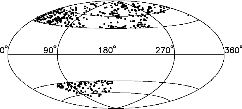
Figure 1: Distribution of the 459 compact groups of our sample in galactic coordinates. The solid line indicating the limit of 40^∘ in galactic latitude is clearly seen.

Seeking to minimize the contamination by stars mistakenly classified as galaxies and resulting in a false group detection, we restricted our sample to CGs with galactic latitude $|b|>40^{\circ}$, resulting in a sample of 459 CGs distributed over 6260 square degrees of the northern sky as shown in Figure 1. Around the north Galactic pole (NGP) there are 352 CGs over 4637 square degrees, while in the southern Galactic cap (SGC) region 107 CGs cover 1623 square degrees. Both regions have similar surface densities of CGs, 0.0759 and 0.0659 groups per square degree, respectively, corroborating the homogeneity of our sample over this large area. In comparison with the sample presented in Iovino et al. (2003), there are 27 groups which are not part of this newer sample due to rejection by the more stringent galactic latitude cutoff (10 groups); improvement of bad areas defined by bright stars and plate defects (see Gal et al. 2004, Lopes et al. 2004) (8 groups); and discarding of a few additional plates which did not meet our final quality standards (9 groups). The catalog consists of 409 groups with 4 members, 47 groups with 5 members, and 3 groups with 6 members.

Table 1 lists the characteristic parameters for sixty CGs representative of our sample. The columns are: (1) group name, composed of PCG (Palomar Compact Group) with the RA and Dec coordinates; (2,3) right ascension and declination (J2000) of the group center; (4) radius of the group in arc minutes; (5) total magnitude of the group, $\rm m_{gr}$, in $r$-band; (6) mean surface brightness of the group in $r$-band; (7) magnitude interval between the brightest and the faintest galaxy in the group, $\Delta{\rm mag}_{\rm comp}$; (8) magnitude interval between the brightest group member and the brightest outlier galaxy within the isolation radius, $\Delta{\rm mag}_{\rm iso}$; and (9) the number of galaxies in the group.

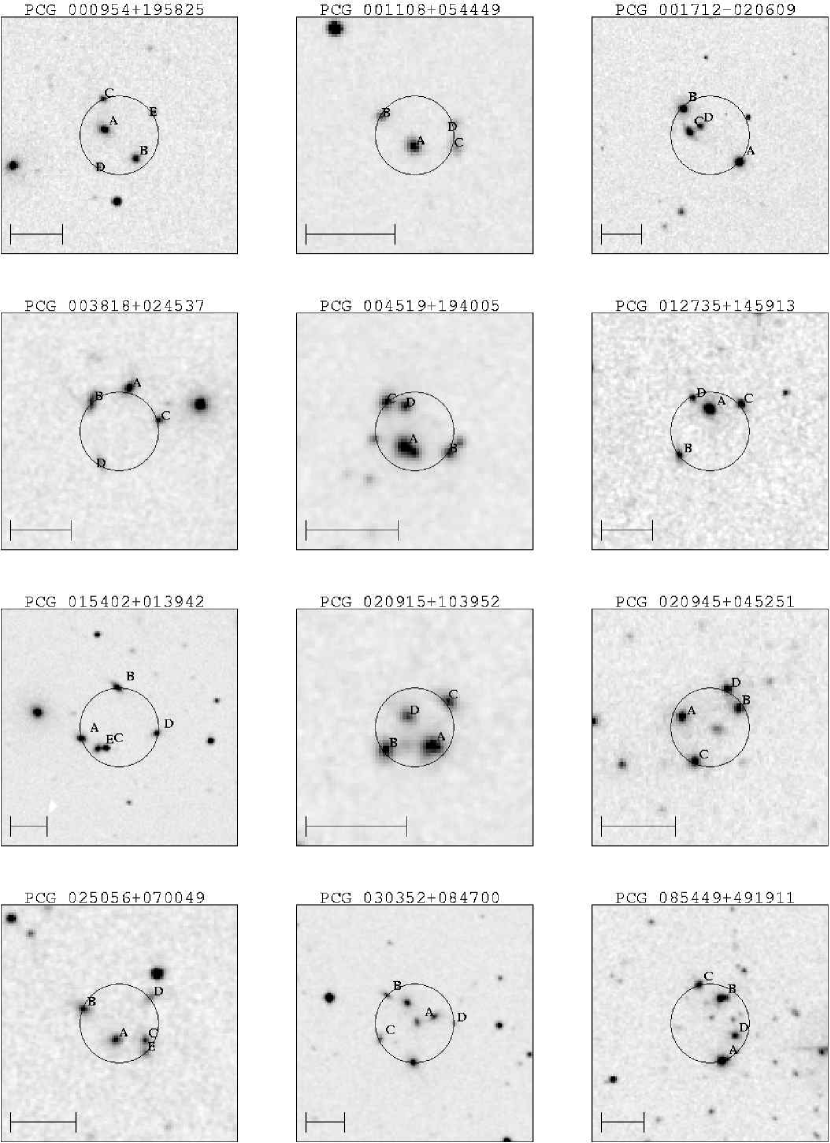
Figure 2: DPOSS (F) images of 60 representative compact group candidates in our sample. The horizontal bar indicates 0.5^′.

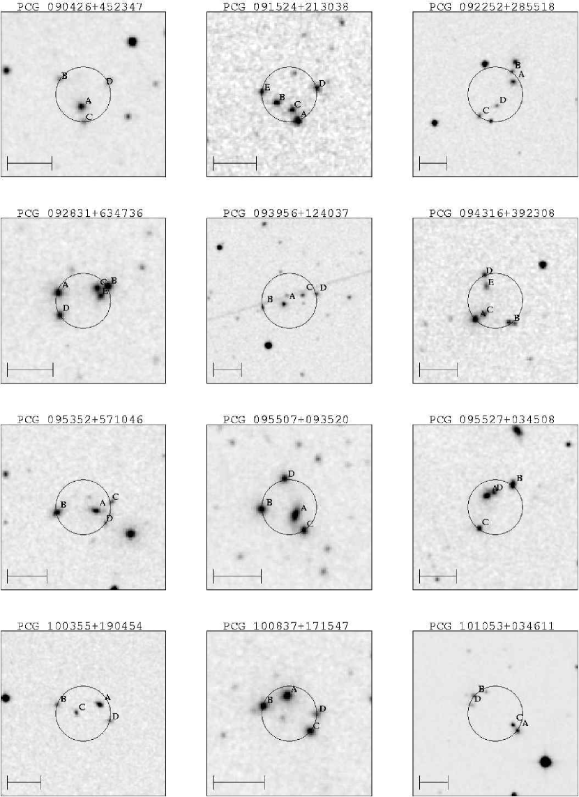
Figure 2: Continued

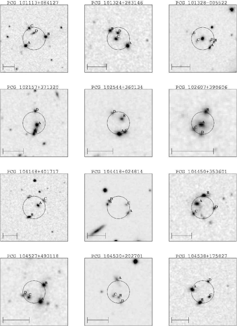
Figure 2: Continued

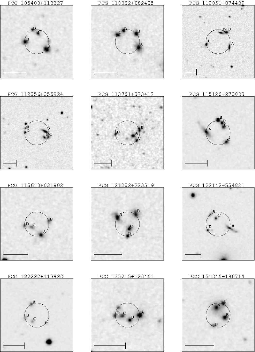
Figure 2: Continued

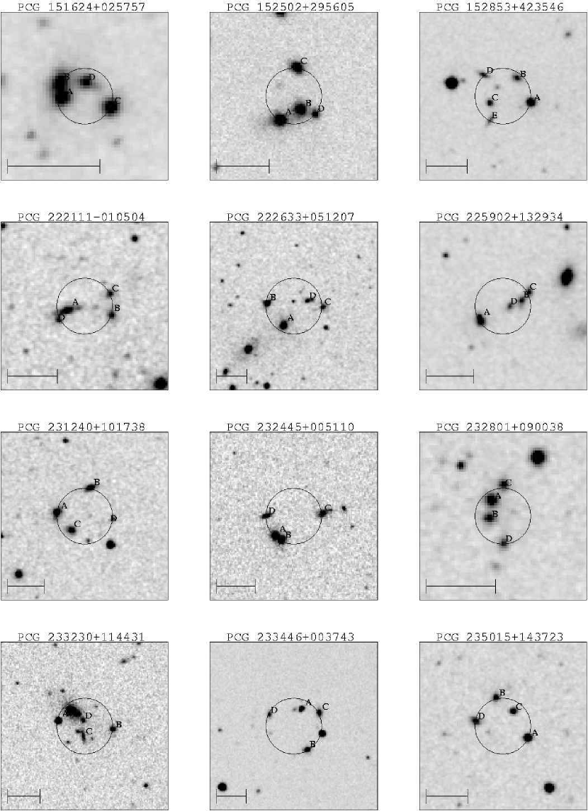
Figure 2: Continued

In Table 2, we list the photometric parameters for each galaxy in these sixty groups in the same order as in Table 1. The columns are: (1) group name, as in Table 1, plus a letter indicating each galaxy in the group, ordered from brightest to faintest; (2,3) right ascension and declination (J2000) for each galaxy in the group; (4) total magnitude in $r$; (5) total color ($g-r$); (6) position angle, in degrees, measured counter-clockwise; (7) ellipticity; and (8) redshift, when it is available in the literature. We distinguish between redshifts available through the SDSS and 2dF databases and those coming from different sources in the NASA Extragalactic Database (NED; we refer the reader to NED Sample Name Information, http://nedwww.ipac.caltech.edu/samples/NEDmdb.html) as the former constitute homogeneous data, and provide access to the spectra as well. Taking the redshifts of all the galaxies available in this table (155 from SDSS and 62 from NED) as representative of the whole sample we estimate a median redshift of $z_{\rm med}$=0.12. The galaxies with available spectra from SDSS are marked to identify those which can be studied in more detail using public data. In Figure 2, we show the DPOSS (F) images of the sixty CGs listed in Tables 1 and 2. The circle indicates the group radius and the horizontal line indicates a length of 0.5^′. The complete catalogs for Tables 1 and 2 with all corresponding finding charts will be published electronically.

Before using this sample for any investigation of the physical nature of CGs we need to understand the selection effects present, which, if not taken into account, can make any conclusion misleading. We examine the global features of this sample using the parameters $\Delta{\rm mag}_{\rm comp}$, $\Delta{\rm mag}_{\rm iso}$, and $\mu_{\rm gr}$, which were used in the sample definition, together with R_gr. The redshift information available for these groups is limited (only 11% of the galaxies, from 145 groups, have spectroscopic redshifts), preventing more detailed analysis of the contamination rate, mass estimates, and studies of dynamical and morphological properties of these systems. However, the available photometric parameters furnish a first glimpse into the reliability of the sample, as representative of a physical class.

The distribution of the parameters noted above are shown in the four panels of Figure 3. In panel (a) we show how the total magnitude of the group varies with group radius. There is large scatter but a majority of the sample is concentrated along the solid line indicating the limiting surface brightness ($\mu_{\rm limit}$=24.0 mag arcsec^-2) imposed as a selection criterion. Also, $\sim$70% of the sample is located between the solid and dashed lines (which represents 1-$\sigma$ of $\theta_{\rm gr}$), a region where the points follow the global trend indicated by the solid line. This trend between total magnitude and size is expected for a sample with a typical physical size and following the flux-distance relation. However, we should emphasize that the concentration of groups towards the solid line is due to the fact that setting a surface brightness limit increases the probability of finding groups with surface brightnesses closer to the border since high surface brightness groups are rarer. Panel (b) shows $\mu_{\rm gr}\times\Delta{\rm mag}_{\rm iso}$. We see a strong concentration of low surface brightness systems, with 56% of the sample having $\mu_{\rm gr}>23.5$. The vertical histogram shows that fainter values of $\mu_{\rm gr}$ are preferred, a consequence of the higher contamination rate for fainter $\mu_{\rm gr}$. Panel (c) shows $\Delta{\rm mag}_{\rm comp}\times\Delta{\rm mag}_{\rm iso}$, with the solid line representing the criterion imposed by the algorithm (${\Delta}\rm mag_{\rm iso}\geq\Delta\rm mag_{\rm comp}+0.5^{\rm m}$). Two effects must be taken into account when examining this figure. First, groups will preferentially have $\Delta{\rm mag}_{\rm comp}$ = 2, close to the criterion limit. Second, groups will tend to have $\Delta{\rm mag}_{\rm iso}$ = 2.5, again near the border of the selection criterion. Finally, in panel (d) the relation between $\mu_{\rm gr}$ and $\Delta{\rm mag}_{\rm comp}$ is plotted. No correlation is present and the absence of groups in the lower left corner of the diagram may indicate a selection effect due to the cutoff in the magnitude of the brightest group member, 16^m. Galaxies in the magnitude interval between 16^m and 16.5^m may be affected by saturation in the plate density measurement, resulting in underestimation of the total magnitude. We note that at these brighter magnitudes ($16\leq\rm m_{\rm r}\leq 17$), comparison with the SDSS database has shown that we miss $\sim$14% of these bright galaxies due to non-detection and misclassification.

3.1 The Space Density of Our Sample

We estimate the space density of the CGs in our sample following the method of Lee et al. (2004, their equation 1), using $z_{\rm med}$ = 0.12, resulting in a value of 1.6$\times$10${}^{-5}h^{3}$ Mpc^-3. If we take the NGP and SGC areas separately we measure space densities of 1.7$\times$10${}^{-5}h^{3}$ Mpc^-3 and 1.5$\times$10${}^{-5}h^{3}$ Mpc^-3, respectively, consistent with the global measure. Lee et al. (2004) reports a value of 9.4$\times$10${}^{-6}h^{3}$ Mpc^-3 when they apply their equation to data from the Iovino et al. (2003) sample, while their estimate for their own sample is 9.0$\times$10${}^{-6}h^{3}$ Mpc^-3 when matching their surface brightness criterion to ours. These estimates are all fully consistent and indicate a space density of $\sim 1.0\times 10^{-5}h^{3}$ Mpc^-3 for CGs in a slightly higher redshift regime.

Mendes de Oliveira & Hickson (1991) found a space density of 3.9$\times$10${}^{-5}h^{3}$ Mpc^-3 for the nearby sample of Hickson groups ($z_{\rm med}=0.03$), which is considerably higher than that measured for the samples mentioned above. Barton et al. (1996) also find a similar space density for nearby CGs, 3.8$\times$10${}^{-5}h^{3}$ Mpc^-3. These two estimates are consistent with each other and were determined using totally different algorithms. If we force the Hickson groups to satisfy our more stringent surface brightness constraint, we find that their space density is reduced to 2.5 $\times$10${}^{-5}h^{3}$ Mpc^-3. Also, a smaller $\Delta{\rm mag}_{\rm comp}$ would further reduce the space density. These results suggest that local CGs have a higher space density compared to their counterparts at higher redshifts, especially considering that $\sim 10\%$ contamination by projection effects may inflate our estimate of the higher redshift space density. However, as pointed out by Lee et al. (2004) there are several possible explanations for this discrepancy. These samples are all based on different criteria which can make such comparisons somewhat meaningless. Thus, it is quite plausible that the discrepancies between nearby and more distant samples reflect only differences in the way various authors defined their search criteria.

4 Groups & Field

In this Section, we investigate some of the group properties compared to the field population, which is defined using the same galaxy catalogs from DPOSS. For each plate catalog we discarded the CGs, as well as galaxies within two Abell radii of clusters found in Gal et al. (2003) and the bad areas where very bright stars heavily contaminate the galaxy catalog (see Gal et al. 2002 for details). We define the field population in the same plates used for the CG catalog, resulting in a magnitude distribution where each bin represents the median counts from all the plates used. Restricting ourselves to the magnitude interval 16$<m_{r}<$19 (where group galaxies are defined) we find that a linear fit to number counts yields a slope of 0.49$\pm$0.01, which is consistent with that obtained by Weir, Djorgovski, & Fayyad (1995b), 0.52$\pm$0.01. This agreement reinforces the characterization of our field population.

To examine whether or not groups are real or merely projection effects, we compare their properties to those of simulated groups composed of field galaxies. These aggregates are created by first searching for relatively isolated galaxies with magnitudes within 0.1 mag of the brightest group galaxies. For each such field galaxy, we then find the nearest four galaxies within 2 magnitudes, which is one of the criteria for the construction of our real group sample. This results in a sample of 36,000 fictitious groups whose properties can statistically be compared to the actual group candidates.

The manner in which mergers proceed at different clustering scales is a longstanding problem in cosmology. In a CG, we can think of inelastic encounters leading to mergers (in some circumstances), and as the cross section of the final product increases the later accretions will occur more rapidly. In this scenario, CGs would evolve into a single galaxy in as short as $\sim$10% of the Hubble time, and we would be faced with the dilemma that they are still observed. In general, merging influences the luminosity function, and thus the difference in brightness between the first and second (or later) ranked galaxies, which can be assessed from statistical measures of $\Delta{\rm mag}_{1-2}$. Numerical simulations have offered interesting insights into this question. Mamon (1987) simulated possible CG merger scenarios and found that $\Delta{\rm mag}_{1-2}$ increases very rapidly with the number of mergers, as we naively expect, becoming quite large even before full coalescence is reached (see his Figure 12). He then applies the Tremaine & Richstone (1977) test to measure how important mergers have been in these systems. Below we describe the results of applying this test to our sample. However, it is important to note that the evolution of $\Delta{\rm mag}_{1-2}$ depends on several CG properties that are currently unknown, including the initial conditions from which the group originated, whether or not the CG resides in a single dark halo or only contains the individual galaxy halos (Mamon 1987), and how dissipation proceeds as the group is formed at an earlier epoch.

Figure 4 shows the distribution of the differences in magnitude between the brightest and the second brightest galaxies ($\Delta{\rm mag}_{1-2}$) in the real groups (solid line) compared to the fictitious groups (dotted line). There is clearly a greater occurrence of lower $\Delta{\rm mag}_{1-2}$ for galaxies in real CGs. For the fictitious systems we find no relation between frequency and $\Delta{\rm mag}_{1-2}$, as expected, since a priori these galaxies do not interact amongst themselves. An additional test was designed in order to better understand the distribution of $\Delta{\rm mag}_{1-2}$. Another fictitious sample was created by randomly selecting galaxies from the actual magnitude distribution of galaxies in real CGs. In this case we computed $\Delta{\rm mag}_{1-2}$ by taking the brightest member galaxy for each of the quartets and a second galaxy randomly selected from the remaining three group members, with $\Delta{\rm mag}_{\rm comp}<$2. This procedure was repeated 20 times for the entire sample to improve the statistics. The dashed line in Figure 4 indicates that the distribution of $\Delta{\rm mag}_{1-2}$ for these fictitious groups differs from the one for real groups. The fact that $\Delta{\rm mag}_{1-2}$ is smaller for real groups than for the fictitious groups suggests that mergers may be the primary mechanism for accreting small mass galaxies onto the most massive ones. Tremaine & Richstone (1977) proposed two measures as evidence for mergers at the bright end, defined as T${}_{1}={\rm rms}(M_{1})/\langle\Delta\rangle$ and T${}_{2}={\rm rms}(\Delta)/(0.677)^{1/2}\langle\Delta\rangle$, where $\Delta$ is the difference in magnitude between the brightest (M₁) and the second brightest galaxy in the group. If mergers are important, then T₁ and T${}_{2}<$1. Mamon (1986) finds T₁=1.16 for 41 Hickson groups with concordant redshifts and suggests that there is no evidence for luminosity function evolution in the Hickson sample. Using the 92 concordant redshift Hickson groups, which include triplets, we find T₂=0.99, corroborating Mamon’s result. In our case, since we do not have redshifts to measure T₁ properly, we have used T₂ instead, and find a value of 0.90$\pm 0.12$, indicating possible mergers for the bright galaxies in our groups. The error quoted for T₂ comes from bootstrapping the sample 1000 times for 90% of the groups, as we expect 10% contamination that might affect the $\Delta$ measurements. We emphasize that this result is merely suggestive, but in combination with other evidence, such as the differing distributions of $\Delta{\rm mag}_{1-2}$ for groups and the field, implies that at least part of this sample should be representative of real structures and not result from projection effects.

Another important piece of information comes from the distribution of $g-r$ colors of the group galaxies. In Figure 5 we present the histograms of colors for galaxies in CGs (solid line) and for field galaxies, where we note a clear excess (5-$\sigma$ considering Poissonian errors) of the former in the interval $0.2<(g-r)<0.5$. Two important points should be noted here: first, the $g-r$ color does not distinguish between early and late type galaxies in the redshift regime of this sample, so we cannot conclude anything about morphological dominance in groups; second, from the figure we can see that the FWHM of the color distribution for group galaxies is approximately a factor of two smaller than the one for field galaxies. Therefore, there seems to be an excess in the central bins of the distribution indicating that there is more color concordance among CG galaxies than among field galaxies, strengthening our view that this sample of groups represents physical entities and not projection effects.

5 Groups and Large Scale Structure

Although little work has been done on modeling and simulating the formation and evolution of compact groups, in the paradigm of hierarchical structure formation we might expect that they form in enhanced density regions and are therefore related to other more significant structures like filaments and clusters (e.g. West 1989, Hernquist, Katz, & Weinberg 1995). In what follows when we refer to the ”relation” between CGs and the LSS we do not attempt any precise definition of it. We basically use angular proximity as a first indicator. In order to quantify the degree of association on firmer grounds we would need a spectroscopic survey complete down to a limiting magnitude that allows a consistent probe of the luminosity function of all observed structures.

Several observational papers addressed the density distribution in the environments of CGs, which is a first approximation of the relation between CGs and other structures in the universe (e.g. Sulentic 1987, Palumbo et al. 1995). They conclude that most of the CGs cannot result from chance alignments. However, the samples available at that time and the subjective nature of their measurements hampered any more serious investigation into how CGs are distributed relative to the LSS. Rood & Struble (1994) and Ramella et al. (1994), following independent ways of establishing such a relation, found that CGs are often embedded in sparser structures. These results were confined to the Hickson sample. More recently, Andernach & Coziol (2004) used the sample of 84 CGs from Iovino et al. (2003) and the cluster sample from Gal et al. (2003) to address this issue and found that 52% of the PCGs in Iovino’s sample are related to clusters. With our sample we can once again examine the CG-LSS association. First, we compare our sample with other catalogs available in the literature through NED. This matching also allows us to show how our automatic search is able to reproduce previous visual searches. Second, we examine the relation between our CG catalog and that of galaxy clusters from Gal et al. (2003).

We performed a preliminary cross-match between our sample and those available in the literature to examine the relation between the groups defined by our objective search and other structures present in the universe, most of which were detected in a subjective manner. Again it is important to bear in mind that association here means angular proximity. Data were collected from NED. We searched for structures including triplets, groups, and clusters within 16.5^′ of our CGs, which corresponds to 1.5 $h^{-1}$Mpc at our estimated median redshift $z_{\rm med}=0.12$. We found that 303 CG candidates (66% of the total sample) are close to at least one other structure, with most of the associations to clusters (69%). Additionally, 28% are found near groups and 3% near triplets. This indicates that the CGs in our sample are to some degree associated with the large scale structure, which is not a surprising result but requires more quantitative assessment. Besides of demonstrating a connection between CGs and the LSS, this comparison has proven valuable in recovering groups previously found by other searches (most of them visually). If we take all the clusters associated with groups and assume that both are at the same redshift, we find a median redshift of $z_{\rm med}$ = 0.14, consistent with the estimate of Iovino et al. (2003) and our estimate for those groups with at least one measured redshift (see Table 2). This makes our catalog the largest and deepest objectively composed sample to date, and together with the work of Lee et al. (2004) based on the SDSS, forms the basis for further studies of this clustering scale.

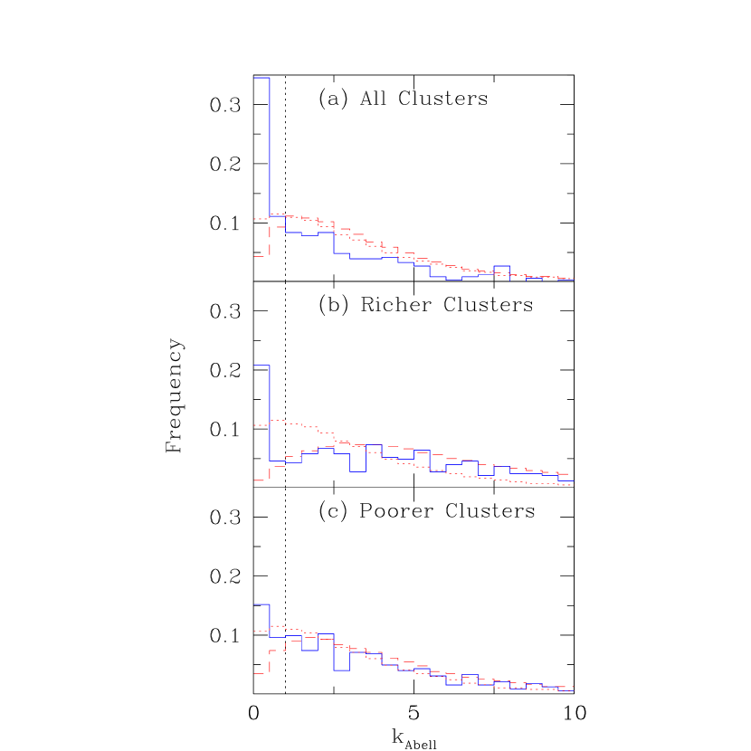
Figure 6: Distributions of the distance to the nearest cluster. As indicated, panels (a), (b), and (c) show the distributions using all clusters in Gal et al. (2003), only rich clusters, and only poor clusters, respectively. Real groups are plotted as the solid line, while the random distributions and the bright galaxies distributions are represented by dashed and dotted lines, respectively.

Considering that NED is a compilation of a wide variety of sources with no homogenization, we require a more homogeneous database to avoid inconsistencies in the way we establish a relation between the CGs and the LSS. The recently published list of galaxy clusters from DPOSS by Gal et al. (2003) provides the most appropriate comparison between CGs in our sample and clusters of galaxies. First, it is drawn from the same galaxy catalog; second, it covers a significant fraction of the northern sky; and finally, it provides important information needed for this comparison, including photometric redshifts and richnesses. We note that Gal et al. (2003) covers only the well-calibrated NGP area to which we restrict our comparison. For each of the 352 CGs in the NGP area we determine the distance to the nearest cluster, expressed as the number of Abell radii at the cluster redshift, k_Abell, shown by the vertical solid line in all panels of Figure 6. Panel (a) shows the distribution of k_Abell as the solid line. We also estimate the distribution of distances to an equal number of points chosen randomly in the same sky region. We repeat this experiment 1000 times, and plot the median distribution of these distances as the dashed line in Figure 6. As a further test, we measure the distance between bright galaxies (16.0$<m_{r}<$17.0) and clusters, selecting 352 galaxies from the NGP area and repeating this search 1000 times. This distance distribution is shown as the dotted lines in Figure 6. All three distributions are normalized by the number of points. As we expect, the distribution of k_Abell for random and bright galaxies are similar, confirming that the strong spatial coincidence between CGs and clusters is not due to our group selection algorithm.

When comparing with all clusters, there is an excess of groups within one Abell radius over the random distribution (32%), in contrast to the percentage we found when comparing to the NED database (66%). Moreover, by dividing the cluster sample by the median richness, we can examine how CGs are related to low and high mass environments, assuming there is a relation between richness and mass (see Bahcall et al. 2003). In panel (b) of Figure 6 we plot the distribution of angular separations between CGs and rich clusters, where only 20% (over random) of the CGs are within one Abell radius, while in panel (c), for poor clusters this percentage drops to 13%. Therefore, we find a marginal excess of CGs related to rich clusters relative to poor clusters. The large excess of small separations in the bright galaxy distribution is due to luminosity segregation in clusters. The important result is that both distributions agree extremely well for ${\rm k_{Abell}}\geq 3.0$. These results uniquely display how CGs are associated with large scale structure. The fact that the distributions for the groups shown in Figure 6 are similar to the expectation for random samples and bright galaxies at ${\rm k_{Abell}}\geq 2.5$ shows that a significant fraction of CGs resides in the low density regions. This is an important clue for scenarios of galaxy formation and evolution, since most of the CGs in our sample do not seem to be associated to either rich or poor clusters.

Using our galaxy database we applied a simple statistical test to study the environment of our CG candidates. As a first test we counted for each group of our sample the density of galaxies ($\rho_{in}$) within $\rm R_{\rm gr}$ in the magnitude range $\rm m_{\rm brightest}<m<m_{\rm brightest}+\Delta\rm mag_{\rm comp}+1.5$ and compared it to the density of galaxies ($\rho_{\rm out}$) in the same magnitude range but in the ring defined by $3\rm R_{\rm gr}<\rm R<15\rm R_{\rm gr}$. Panel (a) of Figure 7 shows the distribution of the ratio $\rho_{\rm in}/\rho_{\rm out}$, or, in other words, the density contrast of CGs in our sample with respect to their immediate neighborhood (having excluded the isolation ring). The vast majority of groups have a density contrast $\rho_{\rm in}/\rho_{\rm out}$ greater than 10 and $\sim 50\%$ greater than 35. This result suggests that CGs in our samples are large overdensities with respect to the local environment, even when disregarding the isolation ring (that, by definition, is empty of galaxies of magnitude comparable to those of the group members).

But how does the local environment of our CG candidates compare to that of a generic galaxy in the database? To answer this question we compared $\rho_{out}$, as defined above, with the same quantity for a generic field galaxy in the database. We considered, for each CG, all galaxies in the database with magnitude within the range $\rm m_{\rm brightest}-0.1^{\rm m}<\rm m<\rm m_{\rm brightest}+0.1^{\rm m}$ and measured the surrounding density using the same prescriptions adopted to measure $\rho_{\rm out}$ for the group. We then calculated for each group the mean value $\rho_{\rm field}$ and its scatter $\sigma_{\rm field}$. Panel (b) of Figure 7 shows the histogram of the quantity $(\rho_{\rm out}-\rho_{\rm field})/\sigma_{\rm field}$. The distribution shows that the vast majority of groups in our sample inhabit regions of density undistinguished from those of the background field distribution. The small tail of groups at values $(\rho_{out}-\rho_{field})/\sigma_{\rm field}>3$ are possibly the few subcondensations within larger structures surviving the selection criteria.

Another important correlation is shown in Figure 8, where we investigate how three important group properties, total magnitude ($\rm m_{gr}$), surface brightness ($\mu_{\rm gr}$), and radius, vary with the distance to the nearest cluster. Data were binned keeping the same number of points in each bin (20), and the error bars are the quartiles of the distribution. We compute the correlation coefficients s (Spearman) and k (Kendall) to show how the parameters are correlated to the distance to the nearest cluster. In principle, if CGs form a truly independent family we should see no correlations. Both correlation coefficients shown in panel (a) indicate a very weak dependence of group surface brightness on k_Abell. Panel (a) also shows that CGs further away from clusters have low surface brightnesses, while those close to clusters cover the entire range in $\mu_{\rm gr}$ with a predominance of low surface brightness CGs. This may indicate that at least a fraction of CGs close enough to clusters might be part of the larger structure responding to the global potential instead of a dynamically independent system. In other words, for k${}_{\rm Abell}<$1.0 the sample could be heavily affected by projection effects. Both correlation coefficients indicate a very weak dependence of group surface brightness on k_Abell. Panel (b) shows no variation of the total magnitude of CGs with k_Abell, demonstrating how difficult it is for an objective algorithm to distinguish between a truly isolated CG and one in the center of a larger structure. Panel (c) shows that the groups’ radii do not vary significantly either. Although in this comparison between both samples (CGs and clusters) there is a strong assumption that CGs are at the same redshift as the angularly nearest cluster, this result suggests that truly compact and isolated systems, as idealized by Hickson, should be found in very low density regimes, although we cannot rule out the possibility that at least a fraction of them reside in sparse groups. Spectroscopic follow-up will be essential to conclusively demonstrate these results.

6 Summary

Searching for small groups over an area of 6260 square degrees around the north and south Galactic caps, using the DPOSS galaxy catalog, we have found 459 CGs expected to be at $z_{\rm med}\sim$0.12 and extending to $z=0.2$. As shown in Iovino et al. (2003) the contamination rate is $\sim$10%, taking into account only projection effects. Although we apply a fairly high cutoff in galactic latitude (40^∘), it is possible that some contamination by stars is still present. This will have to be verified by spectroscopic follow-up, which will allow us not only to remove chance alignment systems but also to address important questions regarding how galaxies evolve in different density regimes.

Although the redshift information available for our sample is not sufficient for a proper dynamical analysis, we are able to address two important questions regarding the nature of CGs. First, we find that the space density of the CGs in our sample (1.6$\times$10${}^{-5}h^{3}$ Mpc^-3) is very similar to that obtained by Lee et al. (2004) for the SDSS CG sample (9.4$\times$10${}^{-6}h^{3}$ Mpc^-3) when applying a similar surface brightness limit. Second, we find that CGs in our sample are associated with clusters at a level of 32%, with a marginal tendency to be more related to rich clusters. This level of association is much lower than that found by previous studies for nearby CGs, such as 75% in Rood & Struble (1994). However, this discrepancy can be due to several reasons, including different ways of establishing the association between CGs and clusters. Rood & Struble (1994) study the association of CGs with not only clusters but also sparse groups, and since these systems dominate the large scale structure in the Universe (Nolthenius & White 1987) it is unsurprising to find a higher rate of association if they are included. Finally, there is no a priori reason to obtain a similar degree of association as we move out in redshift.

Galaxy evolution is already detected at intermediate redshifts $z\sim$0.1-0.2 (the Butcher-Oemler effect, e.g. Butcher & Oemler 1978, Margoniner & de Carvalho 2000, Carlberg et al. 2001). With this objectively selected sample we will be able to establish a firm comparison between predictions and observations, which is one of the most problematic issues in the study of compact groups.

Figure 3: Global properties of the 459 groups in our sample. Correlations between $\rm m_{gr}$, $\mu_{\rm gr}$, $\Delta\rm mag_{\rm comp}$, $\Delta\rm mag_{\rm iso}$, and $\theta_{\rm gr}$ display the limitations of the present sample so that comparison with models are meaningful. In panel (a), the solid line indicates the limiting surface brightness ($\mu_{\rm limit}$=24.0 mag arcsec^-2) imposed as a selection criterion, and together with the dashed line encompasses a region where 70% of the points lie (width of 1-$\sigma$ of $\theta_{\rm gr}$). In panel (c), the solid line represents the criterion ${\Delta}\rm mag_{\rm iso}\geq\Delta\rm mag_{\rm comp}+0.5^{\rm m}$ (see text for details).

Figure 4: Distributions of $\Delta{\rm mag}_{1-2}$ for CGs in our sample (solid line) and the fictitious groups defined from the field population (dotted line) and fictitious groups following the magnitude distribution of the real groups (dashed line). All distributions are normalized to unity.

Figure 5: Distributions of ($g-r$) color for CGs in our sample (solid line) and the fictitious groups representing the field population (dotted line).

Figure 7: Panel (a) exhibits the density contrast of the CGs in our sample wrt to the immediate neighborhood, while in panel (b) we show how the local environment of our CG candidates compares to that of a generic field galaxy, through the quantity $(\rho_{\rm out}-\rho_{\rm field})/\sigma_{\rm field}$ (see text for details).

Figure 8: The correlation between group surface brightness (Panel a), total magnitude (Panel b), and radius (Panel c), and the distance to the nearest cluster (k_Abell). Spearman rank (s) and Kendal (k) correlation coefficients are shown in each panel.

Table 1: Characteristic Parameters of the Groups in our Sample

Name	RA	DEC	Rgr	mgr	$\mu_{\rm gr}$	$\Delta\rm mag_{\rm comp}$	$\Delta\rm mag_{\rm isol}$	Number
	(J2000)	(J2000)	arcmin	mag	$(\rm magarcsec^{-2})$	mag	mag
PCG0009+1958	00 09 54.48	+19 58 25.03	0.380	15.95	23.98	1.834	3.149	5
PCG0011+0544	00 11 8.97	+05 44 49.13	0.222	16.08	22.95	1.819	-	4
PCG0017-0206	00 17 12.53	-02 06 09.22	0.493	15.13	23.73	1.160	1.931	4
PCG0038+0245	00 38 18.24	+02 45 37.62	0.325	16.00	23.69	1.673	2.791	4
PCG0045+1940	00 45 19.32	+19 40 05.99	0.215	15.80	22.60	1.398	-	4
PCG0127+1459	01 27 35.14	+14 59 13.88	0.388	15.84	23.92	1.558	2.524	4
PCG0209+1039	02 09 15.12	+10 39 52.45	0.196	15.51	22.10	1.238	3.289	4
PCG0209+0452	02 09 45.12	+04 52 51.24	0.267	15.56	22.83	0.474	1.496	4
PCG0250+0700	02 50 56.96	+07 00 49.43	0.303	15.62	23.16	1.237	2.612	5
PCG0303+0847	03 03 52.37	+08 47 00.60	0.515	15.13	23.82	1.874	2.616	4
PCG0854+4919	08 54 49.18	+49 19 11.93	0.468	15.27	23.75	1.119	2.282	4
PCG0904+4523	09 04 26.79	+45 23 47.26	0.311	16.28	23.88	1.618	2.228	4
PCG0915+2130	09 15 24.57	+21 30 38.81	0.324	15.81	23.50	1.011	2.588	5
PCG0922+2855	09 22 52.71	+28 55 18.37	0.500	15.31	23.94	1.226	3.170	4
PCG0928+6347	09 28 31.26	+63 47 36.10	0.301	15.27	22.80	0.977	2.574	5
PCG0939+1240	09 39 56.17	+12 40 37.70	0.491	15.01	23.60	0.831	1.558	4
PCG0943+3923	09 43 16.67	+39 23 8.41	0.366	16.05	24.00	1.402	-	5
PCG0953+5710	09 53 52.68	+57 10 47.31	0.350	15.43	23.28	1.842	3.216	4
PCG0955+0935	09 55 7.57	+09 35 20.58	0.290	15.20	22.65	0.946	2.382	4
PCG0955+0345	09 55 27.22	+03 45 8.35	0.376	15.22	23.23	1.181	3.347	4
PCG1003+1904	10 03 55.26	+19 04 54.66	0.411	15.60	23.80	1.453	4.062	4
PCG1008+1715	10 08 37.84	+17 15 47.59	0.269	15.22	22.50	1.366	2.946	4
PCG1010+0346	10 10 53.65	+03 46 12.90	0.480	15.23	23.77	1.235	2.453	4
PCG1011+0841	10 11 13.40	+08 41 27.24	0.492	15.08	23.67	0.950	1.602	4
PCG1013+2831	10 13 24.71	+28 31 47.06	0.295	15.55	23.03	1.100	3.434	4
PCG1013-0055	10 13 28.73	-00 55 22.01	0.309	15.97	23.55	1.601	2.203	5
PCG1021+3713	10 21 57.32	+37 13 20.49	0.277	15.76	23.11	1.123	3.428	4
PCG1025+3601	10 25 44.54	+36 01 34.78	0.220	15.59	22.44	1.847	-	4
PCG1026+3906	10 26 7.76	+39 06 6.37	0.135	15.90	21.69	1.634	3.327	4
PCG1041+4017	10 41 48.68	+40 17 17.23	0.408	15.72	23.91	1.406	3.119	4
PCG1044+0248	10 44 18.96	+02 48 14.44	0.311	15.69	23.29	0.862	-	4
PCG1044+3536	10 44 50.25	+35 36 1.59	0.283	15.00	22.39	1.726	2.245	4
PCG1045+4931	10 45 27.36	+49 31 18.55	0.215	15.61	22.41	1.595	2.332	4
PCG1045+2027	10 45 30.62	+20 27 1.84	0.270	15.61	22.90	1.109	3.690	4
PCG1045+1758	10 45 38.53	+17 58 27.01	0.337	15.63	23.40	1.490	-	4
PCG1054+1133	10 54 0.74	+11 33 27.04	0.260	15.84	23.05	1.522	2.730	4
PCG1100+0824	11 00 2.73	+08 24 35.39	0.254	15.45	22.61	0.982	3.325	4
PCG1120+0744	11 20 51.84	+07 44 39.84	0.520	15.05	23.76	0.280	1.867	4
PCG1123+3559	11 23 56.63	+35 59 24.86	0.470	15.14	23.63	1.915	3.203	5
PCG1137+3234	11 37 1.72	+32 34 12.47	0.347	15.65	23.49	1.056	2.465	4
PCG1151+2738	11 51 20.00	+27 38 3.63	0.266	15.15	22.41	1.866	3.402	5
PCG1156+0318	11 56 10.09	+03 18 2.16	0.246	15.63	22.72	1.436	3.315	4
PCG1212+2235	12 12 52.51	+22 35 19.89	0.216	15.23	22.04	1.212	-	4
PCG1221+5548	12 21 42.14	+55 48 21.60	0.373	15.40	23.39	1.240	2.244	4
PCG1222+1139	12 22 22.05	+11 39 23.26	0.286	15.93	23.35	1.592	2.253	4
PCG1352+1234	13 52 15.45	+12 33 59.83	0.193	16.10	22.66	1.321	1.844	4
PCG1513+1907	15 13 40.07	+19 07 14.12	0.208	15.76	22.48	1.640	-	4
PCG1516+0257	15 16 24.76	+02 57 57.46	0.152	15.25	21.29	0.836	3.117	4
PCG1525+2956	15 25 2.34	+29 56 5.50	0.267	15.11	22.38	1.447	4.186	4
PCG1528+4235	15 28 53.30	+42 35 46.21	0.341	15.74	23.54	1.482	3.617	5
PCG2221-0105	22 21 11.76	-01 05 04.88	0.281	16.26	23.64	1.847	2.731	4
PCG2226+0512	22 26 33.57	+05 12 07.02	0.463	15.44	23.90	1.271	2.189	4
PCG2259+1329	22 59 2.90	+13 29 34.01	0.293	15.74	23.21	1.672	3.824	4
PCG2312+1017	23 12 40.10	+10 17 38.29	0.382	15.71	23.75	1.845	3.619	4
PCG2324+0051	23 24 45.18	+00 51 10.01	0.366	15.61	23.56	1.118	2.216	4
PCG2328+0900	23 28 1.59	+09 00 38.63	0.201	16.02	22.67	1.241	-	4
PCG2332+1144	23 32 30.92	+11 44 31.38	0.432	15.60	23.91	1.537	2.160	4
PCG2334+0037	23 34 46.19	+00 37 43.46	0.477	15.40	23.93	1.010	1.973	4
PCG2350+1437	23 50 15.48	+14 37 23.92	0.336	15.70	23.47	0.844	2.697	4

Table 2: Catalog of Groups

Name	RA	DEC	mr	g-r	PA	Ellip.	z
	(J2000)	(J2000)	mag	mag	$(\circ)$
PCG0009+1958
A	00 09 55.14	+19 58 27.66	16.861	0.341	38.0	0.206
B	00 09 53.83	+19 58 11.21	17.421	0.174	61.4	0.023
C	00 09 55.21	+19 58 45.44	18.174	0.384	$-$70.6	0.053
D	00 09 55.36	+19 58 5.88	18.456	0.382	63.3	0.146
E	00 09 53.15	+19 58 37.85	18.695	0.316	$-$71.2	0.205
PCG0011+0544
A	00 11 9.08	+05 44 44.20	16.811	0.309	86.3	0.203
B	00 11 9.80	+05 44 54.06	17.729	0.514	$-$18.9	0.047
C	00 11 8.14	+05 44 44.16	17.972	0.019	81.1	0.276
D	00 11 8.17	+05 44 51.40	18.630	0.180	2.2	0.177
PCG0017$-$0206
A	00 17 11.09	$-$02 06 29.52	16.323	0.261	33.6	0.007
B	00 17 13.96	$-$02 05 48.88	16.405	0.277	$-$75.6	0.123
C	00 17 13.62	$-$02 06 6.19	16.669	0.088	43.0	0.188
D	00 17 13.07	$-$02 06 2.09	17.483	$-$0.104	$-$9.0	0.160
PCG0038+0245
A	00 38 17.98	+02 45 56.77	16.933	0.361	$-$55.3	0.339
B	00 38 19.20	+02 45 50.62	17.294	0.113	$-$55.6	0.345
C	00 38 16.96	+02 45 41.54	17.793	0.498	$-$8.7	0.047
D	00 38 18.93	+02 45 21.06	18.606	0.113	71.7	0.440
PCG0045+1940
A	00 45 19.61	+19 39 59.94	16.547	0.483	34.6	0.237
B	00 45 18.61	+19 39 57.92	17.669	0.787	$-$45.3	0.499
C	00 45 20.04	+19 40 14.02	17.676	0.392	$-$51.1	0.124
D	00 45 19.61	+19 40 13.01	17.945	0.424	20.6	0.164
PCG0127+1459
A	01 27 35.14	+14 59 25.48	16.610	0.299	57.4	0.119	0.110(sdss)
B	01 27 36.39	+14 58 59.20	17.590	0.207	79.5	0.456
C	01 27 33.89	+14 59 28.57	17.617	0.312	49.2	0.314	0.128(sdss)
D	01 27 35.84	+14 59 32.46	18.168	0.360	63.8	0.292
PCG0154+0139
A	01 54 4.15	+01 39 32.33	16.192	0.406	21.0	0.255
B	01 54 2.13	+01 40 14.99	16.209	0.440	45.0	0.479
C	01 54 2.78	+01 39 24.48	16.380	0.450	2.2	0.124
D	01 53 59.95	+01 39 36.79	16.696	0.484	$-$33.2	0.306
E	01 54 3.20	+01 39 23.94	16.763	0.422	$-$66.1	0.274
PCG0209+1039
A	02 09 14.83	+10 39 46.30	16.350	0.484	$-$9.5	0.153
B	02 09 15.75	+10 39 45.18	17.036	0.416	$-$51.7	0.139
C	02 09 14.50	+10 39 59.72	17.571	0.525	43.1	0.400
D	02 09 15.31	+10 39 55.19	17.588	0.446	79.0	0.205
PCG0209+0452
A	02 09 45.92	+04 52 54.30	16.840	0.618	$-$31.6	0.122
B	02 09 44.39	+04 52 58.44	17.049	0.552	35.1	0.180
C	02 09 45.55	+04 52 36.59	17.138	0.786	38.0	0.190
D	02 09 44.68	+04 53 5.86	17.314	0.475	59.2	0.210
PCG0250+0700
A	02 50 57.13	+07 00 40.72	16.992	0.419	$-$65.1	0.049
B	02 50 58.12	+07 00 55.30	17.050	0.336	28.5	0.290
C	02 50 56.19	+07 00 40.72	17.261	0.394	52.0	0.174
D	02 50 56.00	+07 01 0.59	17.785	0.490	$-$34.8	0.470
E	02 50 56.19	+07 00 35.28	18.229	0.187	47.7	0.171
PCG0303+0847
A	03 03 52.26	+08 47 0.49	16.184	0.212	74.3	0.151
B	03 03 53.90	+08 47 21.55	16.454	0.124	29.0	0.516
C	03 03 54.25	+08 46 47.28	16.578	0.269	$-$77.8	0.264
D	03 03 50.29	+08 46 59.38	18.058	$-$0.057	48.3	0.318
PCG0854+4919
A	08 54 48.39	+49 18 44.96	16.301	0.243	$-$6.9	0.172	0.118(sdss)
B	08 54 48.35	+49 19 28.92	16.518	0.276	$-$24.1	0.244
C	08 54 49.97	+49 19 38.93	17.273	0.552	$-$41.9	0.187	0.184(sdss)
D	08 54 47.41	+49 19 2.56	17.420	0.298	0.6	0.146
PCG0904+4523
A	09 04 26.92	+45 23 38.40	16.917	0.562	$-$77.6	0.021	0.137(sdss)
B	09 04 28.32	+45 23 56.59	18.234	0.658	10.1	0.317
C	09 04 26.72	+45 23 28.64	18.375	0.537	75.2	0.060
D	09 04 25.20	+45 23 55.50	18.535	0.827	$-$49.6	0.414
PCG0915+2130
A	09 15 24.18	+21 30 20.19	16.941	0.622	$-$87.9	0.026
B	09 15 25.22	+21 30 32.69	17.717	0.313	$-$13.1	0.193
C	09 15 24.44	+21 30 27.69	17.751	0.539	$-$25.0	0.107
D	09 15 23.21	+21 30 42.81	17.806	0.529	37.6	0.367
E	09 15 25.96	+21 30 39.96	17.952	0.183	$-$69.2	0.235
PCG0922+2855
A	09 22 51.24	+28 55 31.04	16.179	0.329	30.0	0.327	0.076
B	09 22 51.38	+28 55 42.82	16.944	0.386	$-$44.6	0.213
C	09 22 54.03	+28 54 53.96	17.135	0.253	$-$47.6	0.213
D	09 22 52.59	+28 55 5.52	17.405	0.359	$-$17.6	0.239
PCG0928+6347
A	09 28 33.80	+63 47 42.08	16.639	0.464	30.1	0.118
B	09 28 28.88	+63 47 44.88	16.850	0.605	$-$24.5	0.159
C	09 28 29.91	+63 47 43.77	16.979	0.642	75.1	0.221
D	09 28 33.64	+63 47 27.31	17.278	0.437	$-$51.7	0.085
E	09 28 29.63	+63 47 38.90	17.616	0.375	45.1	0.124
PCG0939+1240
A	09 39 56.62	+12 40 33.49	16.079	1.031	$-$7.4	0.088
B	09 39 58.14	+12 40 31.22	16.610	1.199	$-$79.5	0.385
C	09 39 55.21	+12 40 44.22	16.638	1.193	$-$50.8	0.310
D	09 39 54.21	+12 40 44.22	16.910	1.059	18.0	0.125
PCG0943+3923
A	09 43 18.02	+39 22 53.00	16.980	0.393	$-$50.3	0.104	0.151(sdss)
B	09 43 15.57	+39 22 50.52	18.002	$-$0.025	11.2	0.525
C	09 43 17.42	+39 22 57.15	18.061	0.543	$-$44.2	0.284
D	09 43 17.46	+39 23 28.39	18.201	0.408	$-$74.8	0.105
E	09 43 17.32	+39 23 19.40	18.382	0.055	80.0	0.410
PCG0953+5710
A	09 53 51.59	+57 10 44.72	16.299	0.389	17.2	0.401	0.082(sdss)
B	09 53 55.22	+57 10 43.72	16.541	0.353	$-$20.2	0.222	0.081(sdss)
C	09 53 50.14	+57 10 50.91	17.791	0.365	$-$36.4	0.299
D	09 53 50.74	+57 10 35.77	18.141	0.136	$-$87.7	0.311
PCG0955+0935
A	09 55 7.32	+09 35 15.04	16.242	0.471	$-$75.1	0.489
B	09 55 8.74	+09 35 18.92	16.659	0.501	45.5	0.129
C	09 55 6.96	+09 35 5.71	16.990	0.389	47.4	0.072
D	09 55 7.77	+09 35 37.72	17.188	0.453	$-$60.5	0.094
PCG0955+0345
A	09 55 27.70	+03 45 17.39	16.243	0.322	$-$38.8	0.340	0.091(sdss)
B	09 55 26.29	+03 45 26.10	16.594	0.050	$-$80.7	0.239
C	09 55 28.14	+03 44 50.57	16.971	0.313	12.2	0.232	0.094(sdss)
D	09 55 27.34	+03 45 19.76	17.424	0.065	0.9	0.200
PCG1003+1904
A	10 03 54.22	+19 05 2.11	16.387	0.365	34.1	0.271
B	10 03 56.92	+19 05 2.11	17.232	0.336	48.2	0.075
C	10 03 55.70	+19 04 55.09	17.553	0.368	56.6	0.312
D	10 03 53.61	+19 04 47.21	17.840	0.296	12.4	0.264
PCG1008+1715
A	10 08 37.99	+17 15 57.17	16.247	0.569	23.4	0.010
B	10 08 38.94	+17 15 51.12	16.495	0.594	$-$24.4	0.421	0.121
C	10 08 37.01	+17 15 36.61	16.992	0.594	19.5	0.071
D	10 08 36.71	+17 15 46.95	17.613	0.385	$-$35.5	0.234
PCG1010+0346
A	10 10 52.16	+03 45 54.83	16.298	0.013	75.3	0.162	0.028(sdss)
B	10 10 55.15	+03 46 31.01	16.684	0.303	55.2	0.056	0.095(sdss)
C	10 10 52.47	+03 46 0.77	16.774	0.574	76.4	0.134
D	10 10 55.38	+03 46 22.04	17.533	0.006	11.9	0.379	0.104(sdss)
PCG1011+0841
A	10 11 14.92	+08 41 8.12	16.208	0.286	$-$18.0	0.313	0.097(sdss)
B	10 11 11.43	+08 41 31.09	16.356	0.137	11.1	0.079
C	10 11 14.29	+08 41 53.63	16.853	0.106	63.7	0.187
D	10 11 13.53	+08 41 40.70	17.158	$-$0.005	$-$24.1	0.616
PCG1013+2831
A	10 13 23.69	+28 31 35.55	16.579	0.436	69.1	0.184
B	10 13 25.74	+28 31 58.55	17.047	0.444	61.0	0.153
C	10 13 25.06	+28 31 46.13	17.166	0.504	19.9	0.281
D	10 13 24.89	+28 31 55.23	17.679	0.393	11.1	0.192
PCG1013$-$0055
A	10 13 28.02	$-$00 55 37.09	16.780	0.062	$-$66.3	0.521
B	10 13 27.57	$-$00 55 28.34	18.002	0.507	$-$83.5	0.203
C	10 13 29.46	$-$00 55 27.37	18.148	0.324	88.8	0.430
D	10 13 27.96	$-$00 55 26.54	18.187	0.795	$-$66.7	0.254
E	10 13 29.89	$-$00 55 15.71	18.381	$-$0.139	35.2	0.385
PCG1021+3713
A	10 21 57.03	+37 13 16.54	16.723	0.546	86.6	0.322
B	10 21 57.42	+37 13 3.90	17.393	0.382	$-$42.6	0.102
C	10 21 57.29	+37 13 8.26	17.422	0.426	82.0	0.309
D	10 21 57.23	+37 13 37.12	17.846	0.426	78.0	0.292
PCG1025+3601
A	10 25 44.47	+36 01 21.86	16.317	0.193	2.2	0.138
B	10 25 44.23	+36 01 39.98	17.061	0.923	84.1	0.107
C	10 25 43.95	+36 01 23.81	17.826	$-$0.204	$-$43.6	0.345
D	10 25 45.14	+36 01 45.80	18.164	0.990	37.5	0.170
PCG1026+3906
A	10 26 7.91	+39 06 5.03	16.708	0.421	6.2	0.235
B	10 26 7.61	+39 06 14.29	17.389	0.458	87.8	0.094
C	10 26 8.33	+39 06 1.88	17.881	0.601	77.3	0.292
D	10 26 7.91	+39 05 58.46	18.342	0.232	35.8	0.096
PCG1041+4017
A	10 41 48.02	+40 17 21.08	16.734	0.253	32.7	0.168	0.069
B	10 41 49.64	+40 16 55.30	16.788	0.091	$-$16.1	0.455
C	10 41 46.95	+40 17 31.64	17.972	0.092	40.0	0.525
D	10 41 49.92	+40 17 37.24	18.140	0.523	32.4	0.247
PCG1044+0248
A	10 44 17.91	+02 48 4.32	16.870	$-$0.115	$-$72.7	0.290
B	10 44 20.17	+02 48 18.97	16.887	$-$0.146	$-$68.0	0.163
C	10 44 18.08	+02 48 18.04	17.542	0.498	38.4	0.131	0.123(sdss)
D	10 44 20.01	+02 48 24.59	17.732	0.720	$-$8.7	0.202
PCG1044+3536
A	10 44 50.95	+35 36 6.30	16.021	$-$0.071	45.6	0.350	0.051
B	10 44 50.05	+35 36 18.40	16.052	0.332	$-$3.4	0.534
C	10 44 51.40	+35 35 51.97	17.066	0.529	$-$58.8	0.108
D	10 44 48.87	+35 35 59.21	17.747	0.313	$-$62.9	0.224
PCG1045+4931
A	10 45 26.76	+49 31 7.03	16.446	0.565	$-$83.8	0.107	0.173(sdss)
B	10 45 26.25	+49 31 25.68	17.005	0.511	77.9	0.191
C	10 45 28.12	+49 31 12.76	17.632	0.515	43.9	0.208	0.168(sdss)
D	10 45 28.65	+49 31 15.60	18.041	0.531	$-$29.7	0.594
PCG1045+2027
A	10 45 30.79	+20 27 17.82	16.520	0.326	65.7	0.512
B	10 45 30.67	+20 26 53.09	17.267	0.276	$-$0.5	0.074
C	10 45 31.19	+20 26 55.07	17.418	0.173	44.4	0.152
D	10 45 30.45	+20 26 45.82	17.629	0.276	36.3	0.162
PCG1045+1758
A	10 45 39.91	+17 58 31.48	16.647	0.231	2.5	0.340
B	10 45 38.98	+17 58 7.86	16.651	0.290	$-$32.6	0.245
C	10 45 37.78	+17 58 17.55	17.940	0.255	$-$37.9	0.333
D	10 45 37.90	+17 58 45.16	18.137	0.312	48.6	0.302
PCG1054+1133
A	10 53 59.93	+11 33 16.89	16.697	0.072	30.2	0.088
B	10 54 1.79	+11 33 26.28	17.139	0.246	60.2	0.107
C	10 54 0.69	+11 33 36.76	18.022	0.464	40.8	0.379
D	10 54 1.15	+11 33 41.40	18.219	0.102	38.0	0.154
PCG1100+0824
A	11 00 1.85	+08 24 27.47	16.493	0.065	70.0	0.318
B	11 00 2.03	+08 24 44.71	17.040	0.410	68.8	0.190
C	11 00 3.61	+08 24 43.31	17.058	0.263	23.3	0.215	0.073(sdss)
D	11 00 3.11	+08 24 48.28	17.475	0.297	57.0	0.067
PCG1120+0744
A	11 20 49.96	+07 44 25.98	16.446	0.184	$-$86.1	0.634
B	11 20 50.48	+07 45 3.67	16.458	0.407	0.5	0.293
C	11 20 53.88	+07 44 32.78	16.583	0.437	$-$59.6	0.296
D	11 20 51.38	+07 45 2.30	16.726	0.286	7.4	0.652
PCG1123+3559
A	11 23 55.11	+35 59 28.14	16.069	0.085	24.4	0.662
B	11 23 55.17	+35 59 13.88	16.728	0.075	43.8	0.394
C	11 23 54.45	+35 59 15.00	17.218	0.342	$-$7.6	0.282
D	11 23 58.86	+35 59 24.36	17.375	0.308	68.2	0.060
E	11 23 58.80	+35 59 34.73	17.984	0.297	$-$13.8	0.486
PCG1137+3234
A	11 37 0.94	+32 34 6.45	16.778	0.617	12.9	0.190
B	11 37 0.11	+32 34 16.90	16.944	0.495	83.5	0.318
C	11 37 0.48	+32 33 58.72	17.389	0.740	88.3	0.250
D	11 37 3.35	+32 34 9.55	17.834	0.491	$-$38.2	0.453
PCG1151+2738
A	11 51 21.21	+27 38 3.80	16.214	0.015	47.3	0.611
B	11 51 20.07	+27 38 19.57	16.585	0.211	$-$81.2	0.118
C	11 51 19.25	+27 37 51.17	17.144	0.313	$-$13.7	0.042
D	11 51 19.69	+27 38 15.72	17.372	0.397	61.5	0.218
E	11 51 19.54	+27 38 10.64	18.080	0.113	70.2	0.365
PCG1156+0318
A	11 56 9.76	+03 17 48.70	16.298	0.111	39.3	0.288
B	11 56 9.11	+03 18 4.97	17.577	0.249	87.6	0.294
C	11 56 10.50	+03 17 57.73	17.665	0.231	16.4	0.394	0.072(sdss)
D	11 56 11.05	+03 17 59.35	17.734	0.173	$-$54.9	0.133
PCG1212+2235
A	12 12 53.31	+22 35 26.55	16.393	0.147	48.5	0.409
B	12 12 51.93	+22 35 30.08	16.460	0.056	35.3	0.116
C	12 12 52.42	+22 35 14.28	16.877	0.435	$-$59.1	0.161
D	12 12 52.55	+22 35 6.94	17.605	0.396	$-$88.8	0.232
PCG1221+5548
A	12 21 39.72	+55 48 12.38	16.236	0.180	30.2	0.727	0.044
B	12 21 43.67	+55 48 39.85	17.131	0.193	$-$49.8	0.643
C	12 21 42.56	+55 48 32.37	17.227	0.363	66.6	0.099	0.034(sdss)
D	12 21 44.51	+55 48 11.52	17.476	0.316	5.4	0.132
PCG1222+1139
A	12 22 22.60	+11 39 38.38	16.860	0.461	$-$47.7	0.066
B	12 22 23.18	+11 39 19.33	17.427	0.613	$-$60.9	0.245
C	12 22 22.49	+11 39 14.26	17.536	0.494	87.5	0.150
D	12 22 21.19	+11 39 11.52	18.452	0.245	34.5	0.271
PCG1352+1233
A	13 52 14.66	+12 34 0.19	16.978	0.388	24.4	0.076
B	13 52 15.28	+12 33 55.19	17.633	0.391	$-$7.3	0.082
C	13 52 15.77	+12 33 59.18	17.935	0.392	$-$9.1	0.273
D	13 52 16.24	+12 33 59.47	18.299	0.314	$-$57.0	0.144
PCG1513+1907
A	15 13 40.26	+19 07 21.65	16.734	$-$0.050	$-$14.6	0.080
B	15 13 39.61	+19 07 11.67	17.187	0.238	2.5	0.134
C	15 13 39.76	+19 07 25.75	17.332	0.461	65.5	0.031
D	15 13 40.39	+19 07 2.49	18.374	0.297	$-$10.4	0.351
PCG1516+0257
A	15 16 25.25	+02 57 56.59	16.512	0.623	$-$80.8	0.314
B	15 16 25.31	+02 58 1.31	16.548	0.633	$-$87.4	0.208	0.113(sdss)
C	15 16 24.20	+02 57 53.60	16.768	0.593	$-$42.7	0.139
D	15 16 24.75	+02 58 1.60	17.348	0.492	20.2	0.337
PCG1525+2956
A	15 25 2.97	+29 55 51.78	16.221	0.314	$-$6.5	0.225
B	15 25 2.04	+29 55 56.96	16.388	0.395	69.6	0.072
C	15 25 2.21	+29 56 21.41	16.670	0.541	25.7	0.230
D	15 25 1.41	+29 55 54.98	17.668	0.622	12.3	0.050
PCG1528+4235
A	15 28 51.54	+42 35 40.05	16.717	0.372	$-$16.7	0.130
B	15 28 52.36	+42 35 58.17	17.559	0.286	27.1	0.273
C	15 28 54.19	+42 35 40.96	17.748	0.208	39.5	0.186
D	15 28 54.58	+42 36 1.04	17.872	0.304	20.5	0.465
E	15 28 54.20	+42 35 28.35	18.199	0.273	$-$63.0	0.555
PCG2221$-$0105
A	22 21 12.42	$-$01 05 6.40	16.950	0.358	$-$23.4	0.567	0.107(sdss)
B	22 21 10.68	$-$01 05 9.46	17.912	0.819	$-$86.5	0.279
C	22 21 10.74	$-$01 04 57.36	18.274	0.794	$-$26.9	0.214
D	22 21 12.76	$-$01 05 12.44	18.797	0.418	57.5	0.173
PCG2226+0512
A	22 26 34.35	+05 11 47.40	16.346	0.206	$-$56.3	0.183
B	22 26 35.43	+05 12 8.57	16.785	0.332	$-$52.4	0.211
C	22 26 31.71	+05 12 5.47	17.579	$-$0.053	60.6	0.165
D	22 26 32.72	+05 12 11.56	17.617	0.281	$-$14.4	0.503
PCG2259+1329
A	22 59 3.95	+13 29 25.40	16.467	0.467	55.9	0.187	0.129(sdss)
B	22 59 2.16	+13 29 37.46	17.408	0.441	$-$59.4	0.357
C	22 59 1.85	+13 29 42.61	17.736	0.251	83.1	0.197
D	22 59 2.66	+13 29 33.90	18.139	0.268	$-$37.8	0.292
PCG2312+1017
A	23 12 41.65	+10 17 40.77	16.668	0.333	$-$61.4	0.249
B	23 12 39.79	+10 18 0.76	17.104	0.331	$-$13.8	0.517
C	23 12 40.88	+10 17 26.63	17.260	0.271	13.7	0.143
D	23 12 38.56	+10 17 35.34	18.513	$-$0.096	$-$50.8	0.309
PCG2324+0051
A	23 24 46.17	+00 50 54.46	16.636	0.423	50.0	0.114
B	23 24 45.83	+00 50 50.35	17.131	0.369	$-$56.8	0.426
C	23 24 43.73	+00 51 11.70	17.242	0.231	$-$19.2	0.438
D	23 24 46.65	+00 51 9.76	17.754	0.475	$-$18.7	0.516	0.119(sdss)
PCG2328+0900
A	23 28 1.94	+09 00 44.42	16.912	0.431	36.0	0.068
B	23 28 1.99	+09 00 36.97	17.605	0.489	$-$25.0	0.164
C	23 28 1.59	+09 00 50.72	17.835	0.390	$-$9.7	0.030
D	23 28 1.58	+09 00 26.57	18.153	0.364	$-$77.6	0.265
PCG2332+1144
A	23 32 32.66	+11 44 35.70	16.448	0.368	$-$88.5	0.050
B	23 32 29.18	+11 44 27.05	17.245	0.486	$-$66.2	0.169
C	23 32 31.06	+11 44 20.69	17.278	0.043	78.8	0.624
D	23 32 31.06	+11 44 35.99	17.985	0.389	49.2	0.388
PCG2334+0037
A	23 34 45.71	+00 38 0.46	16.655	0.351	$-$66.6	0.183
B	23 34 45.37	+00 37 17.65	16.778	0.274	$-$30.0	0.112
C	23 34 44.49	+00 37 56.39	16.817	0.351	87.8	0.259	0.086(sdss)
D	23 34 47.95	+00 37 54.30	17.665	0.181	$-$87.2	0.350
PCG2350+1437
A	23 50 14.27	+14 37 14.20	16.665	0.654	$-$2.4	0.055
B	23 50 15.82	+14 37 43.47	17.421	0.647	$-$87.6	0.075
C	23 50 14.97	+14 37 33.46	17.501	0.935	2.6	0.191
D	23 50 16.86	+14 37 26.65	17.509	0.182	17.4	0.254	0.201(sdss)

References

- (1) Andernach, H., & Coziol, R. 2004, in Nearby Large-Scale Structures and the Zone of Avoidance, eds. Fairall, A.P., Woudt, P. ASP Conf Series, San Francisco, in press
- (2) Athanassoula, E. 2000, in Small Galaxy Groups: IAU Colloquium 174, eds. Valtonen, M.J., Flynn, C. ASP Conf. Series, Volume 209 (San Francisco: ASP), p. 245
- (3) Bahcall et al. 2003, ApJ, 585, 182
- (4) Barnes, J. 1985, MNRAS, 215, 517
- (5) Barnes, J. 1989, Nature, 338, 123
- (6) Barton et al. 1996, AJ, 112, 871
- (7) Butcher, H., & Oemler, A.Jr. 1978, ApJ, 226, 559
- (8) Carlberg, R. 2001, ApJ, 563, 736
- (9) Coziol et al. 1998a, ApJ, 493, 563
- (10) Coziol et al. 1998b, ApJ, 506, 545
- (11) Coziol, R., Iovino, A., & de Carvalho, R.R. 2000, AJ, 120, 47
- (12) Coziol, R., Brinks, E., & Bravo-Alfaro, H. 2004, AJ, 128, 68
- (13) de Carvalho et al. 1997, ApJS, 110, 1
- (14) de la Rosa, I.G., de Carvalho, R.R., & Zepf, S.E. 2001a, AJ, 122, 93
- (15) de la Rosa, I.G., Coziol, R., de Carvalho, R.R., & Zepf, S.E. 2001b, Ap&SS, 276, 717
- (16) Diaferio, A., Geller, M.J., & Ramella, M. 1994, AJ, 107, 668
- (17) Djorgovski, S.G., Gal, R., Odewahn, S., de Carvalho, R., Brunner, R., Longo, G., & Scaramella, R. 1999, in Wide Field Surveys in Cosmology, eds. S. Colombi, Y. Mellier, & B. Raban, Gif sur Yvette: Editions Frontières, p. 89.
- (18) Fayyad, U. 1991, PhD Thesis, EECS Department, The University of Michigan
- (19) Kelm, B., & Forcardi, P. 2004, A&A, 418, 937
- (20) Kelm, B., Focardi, P., & Zitelli, V. 2004, A&A, 418, 25
- (21) Gal, R. 2002, PhD Thesis, California Institute of Technology
- (22) Gal et al. 2003, AJ, 125, 2064
- (23) Gal et al. 2004, AJ, 128, 3082
- (24) Governato, F. et al. 1991, ApJ, 371L, 15
- (25) Helsdon, S.F., & Ponman, T.J. 2000a, MNRAS, 315, 356
- (26) Helsdon, S.F., & Ponman, T.J. 2000b, MNRAS, 319, 933
- (27) Hernquist, L., Katz, N., & Weinberg, D.H. 1995, ApJ, 442, 57
- (28) Hickson, P. 1982, ApJ, 255, 382
- (29) Hickson, P. 1992, ApJ, 399, 353
- (30) Hickson, P. 1997, ARA&A, 35, 357
- (31) Iovino, A. 2002, AJ, 124, 2471
- (32) Iovino et al. 2003, AJ, 125, 1660
- (33) Jones et al. 2003, MNRAS, 343, 627
- (34) Lee et al. 2004, AJ, 127, 1811
- (35) Lopes et al. 2004, AJ, 128, 1017
- (36) Mamon, G.A. 1986, ApJ, 307, 426
- (37) Mamon, G.A. 1987, ApJ, 321, 622
- (38) Margoniner, V.E., & de Carvalho, R.R. 2000, AJ, 119, 1562
- (39) Mendes de Oliveira, C., & Hickson, P. 1991, ApJ, 380, 30
- (40) Nolthenius, R., & White, S.D.M. 1987, MNRAS, 225, 505
- (41) Odewahn, S. et al. 1992, AJ, 103, 318
- (42) Odewahn, S. et al. 2004, AJ, 128, 3092
- (43) Palumbo et al. 1995, AJ, 109, 1476
- (44) Phillips et al. 1986, AJ, 91, 1062
- (45) Plionis, M., Basilakos, S., & Tovmassian, H.M. 2004, MNRAS, 352, 1323
- (46) Ponman et al. 1994, Nature, 369, 462
- (47) Prandoni et al. 1994, AJ, 107, 1235
- (48) Proctor et al. 2004, MNRAS, 349, 1381
- (49) Ramella et al. 1994, AJ, 107, 1623
- (50) Ribeiro et al. 1998, ApJ, 497, 72
- (51) Rood, H.J., & Struble, M.F. 1994, PASP, 106, 403
- (52) Rose, J.A. 1977, ApJ, 211, 311
- (53) Rose, J.A. 1979, ApJ, 231, 10
- (54) Seyfert, C.K. 1948, AJ, 53, 203
- (55) Schmitt, H. 2001, AJ, 122, 2243
- (56) Shimada et al. 2000, AJ, 119, 2664
- (57) Stephan, M. 1877, MNRAS, 37, 334
- (58) Sulentic, J.W. 1987, ApJ, 322, 605
- (59) Tremaine, S.D., & Richstone, D.O. 1977, ApJ, 212, 311
- (60) Weir, N., Djorgovski, S.G., & Fayyad, U. 1995a, AJ, 109, 2401
- (61) Weir, N., Djorgovski, S.G., & Fayyad, U. 1995b, AJ, 110, 1
- (62) Weir, N., Djorgovski, S.G., Fayyad, U., & Roden, J. 1995c, PASP, 107, 1243
- (63) West, M.J. 1989, ApJ, 344, 535
- (64) Zabludoff, A.I., & Mulchaey, J.S. 1998, ApJ, 498L, 5
- (65) Zhen, J., Valtonen, M.J., & Chernin, A.D. 1993, AJ, 105, 2047