Inferences from pulsational amplitudes and phases for multimode $\delta$ Sct star FG Vir

We combine photometric and spectroscopic data on twelve modes excited in FG Vir to determine their spherical harmonic degrees, $\ell$, and to obtain constraints on the star model. The effective temperature consistent with the mean colours and the pulsation data is about 7200K. In six cases, the $\ell$ identification is unique with above 80 % probability. Two modes are identified as radial. Simultaneously with $\ell$, we determine a complex parameter $f$ which probes subphotospheric stellar layers. Comparing its values with those derived from models assuming different treatment of convection, we find evidence that convective transport in the envelope of this star is inefficient.

1 Introduction

FG Vir is the most studied $\delta$ Sct star. After the Sun it is the Main Sequence star with the largest number of eigenfrequencies measured. In spite of efforts (e.g. Breger et al. 1995, Guzik & Bradley 1995, Viskum et al. 1998, Breger et al. 1999, Templeton et al. 2001 ), we still do not have a good seismic model of this object. Not much has been learnt so far from this rich frequency data. The main obstacle is the lack of revealing features in the oscillation spectrum. For a few dominant peaks identification of the spherical harmonic degree, $\ell$, have been suggested. However, even with this few $\ell$ values the task of disentangling the spectrum appears formidable. It is frustrating that so far the progress in amplitude resolution resulting in ever growing number of detected modes does not help. It seems that the science will be served better if we focus on information contained in a few peaks for which we have reliable information on amplitudes and phases of the light variation in various photometric passbands as well as of the radial velocity variation. The problem with low-amplitude peaks is that, rather than just representing missing component of low-degree multiplets, they may also correspond to moderate-degree modes of unknown azimuthal order.

The identification of $\ell$ values is of the highest priority as a first step towards a unique mode identification. The most widely used tool for $\ell$ determination has been the amplitude ratio vs. phase differences diagrams in two passbands.

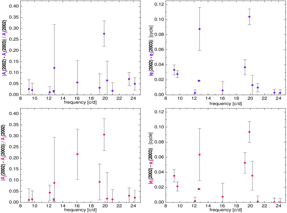
Figure 1: Changes in the observed photometric amplitudes (left panels) and phases (right panels) of FG Vir light curves between the 2002 and 2003 seasons. The upper panels are for the $v$ Strömgren passband and the lower panels are for the $y$ passband.

The usefulness of these diagrams is limited because mode localization depends not only on $\ell$ but also on a certain complex parameter describing the relative perturbation of the bolometric flux. The parameter, which we denote $f$, may be determined by solving the linear nonadiabatic oscillation problem for the stellar model. Unfortunately, the calculated $f$ values are unreliable because they depend on stellar parameters and, more importantly, on the treatment of convection. In this paper, we follow an alternative approach (Daszyńska-Daszkiewicz, Dziembowski, Pamyatnykh, 2003 (Paper I), 2004), which does not require any assumptions about convection because $f$ is determined together with $\ell$ from observations. The inferred value of $f$ is of interest in itself.

The determination of $\ell$ and $f$ values from pulsation amplitudes and phases requires atmospheric models calculated for the star mean photospheric parameters. Nonetheless, we still call such $f$’s empirical. There is an uncertainty in these parameters, which must be taken into account, but it is far less severe than in the theoretical $f$’s derived as solutions of the linear nonadiabatic oscillation problem.

A comparison of the empirical and theoretical $f$’s yields a new seismic probe. The value of $f$ is determined in the layers, where the thermal time scale is of the order of pulsation period. These are subphotospheric layers and they are poorly probed by frequencies. Thus, $f$’s must be regarded as a supplementary probe of star interiors.

Our paper is constructed as follows. In Sect. 2. we review recent observational data on FG Vir. Identification of the spherical harmonic degrees, $\ell$, as well as the $f$ values for twelve dominant modes in the oscillation spectrum is presented in Sect. 3. Constraints on models of convection based on the $f$ values are derived in Sect. 4.

2 Observations

Three recent, extensive photometric campaigns on FG Vir were undertaken in the years 2002, 2003 and 2004 by the Delta Scuti Network (Breger et al. 2003, 2005), while spectroscopic observations were obtained in 2002. For the analysis undertaken in this paper, we have only used the photometric data from 2002, rather than adopting the combined 2002–2004 solution, which has lower observational uncertainties. The reason is presented in Fig. 1, which demonstrates that small year-to-year changes in the amplitudes and phases may exist. Such changes might be intrinsic to the star due to amplitude variability or observational due to missing frequencies of low amplitude. In spite of some annual amplitude and phase variability, the amplitude ratios, $A_{v}/A_{y}$, and phase shifts, $\varphi_{v}-\varphi_{y}$, show no annual variations beyond the statistical uncertainties expected from the calculated photometric errors. Thus, the amplitude and phase variability does not affect the mode identification. In Fig. 2 we present amplitude ratio vs. phase difference diagrams, which have been traditionally used for mode degree identification. For certain modes, we see significant differences in the positions determined from the 2002 and 2003 data. Indeed, if there are amplitude and/or phase changes, we may obtain an incorrect result for $\ell$ from data which are not simultaneous. It appears safer to rely only on the photometric and spectroscopic data obtained during 2002.

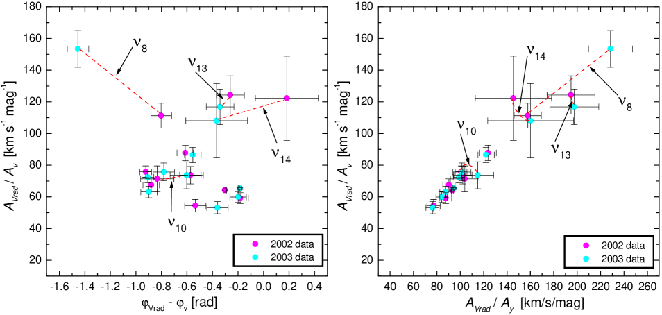
Figure 2: The amplitude ratio vs. phase difference diagram (left panel) and the amplitude ratio vs. amplitude ratio diagram (right panel) for the dominant modes in FG Vir oscillation spectrum. The diagrams are based on the radial velocity data taken in 2002 and the two seprate sets of photometric data taken in 2002 and 2003.

3 Inferring $\ell$ and $f$ from observations

3.1 The method

The method is described in detail in Paper I. Here we give only a brief outline.

The complex photometric amplitudes for a number of passbands, $\lambda$, are written in the form of the following set of linear observational equations

$${\cal D}_{\ell}^{\lambda}({\tilde{\varepsilon}}f)+{\cal E}_{\ell}^{\lambda}{\tilde{\varepsilon}}=A^{\lambda},$$ (1)

where

$${\tilde{\varepsilon}}=\varepsilon Y^{m}_{\ell}(i,0),$$ (2)

$${\cal D}_{\ell}^{\lambda}=\frac{1}{4}b_{\ell}^{\lambda}\frac{\partial\log({\cal F}_{\lambda}|b_{\ell}^{\lambda}|)}{\partial\log T_{\rm{eff}}}$$ (3)

$${\cal E}_{\ell}^{\lambda}=b_{\ell}^{\lambda}\left[(2+\ell)(1-\ell)-\left(\frac{\omega^{2}R^{3}}{GM}+2\right)\frac{\partial\log({\cal F}_{\lambda}|b_{\ell}^{\lambda}|)}{\partial\log g}\right]$$ (4)

Having spectroscopic observations we can supplement the above set with the expression for the radial velocity (the first moment, ${\cal M}_{1}^{\lambda}$)

$${\rm i}\omega R\left(u_{\ell}^{\lambda}+\frac{GM}{R^{3}\omega^{2}}v_{\ell}^{\lambda}\right){\tilde{\varepsilon}}={\cal M}_{1}^{\lambda}$$ (5)

Symbols in Eqs. (1)$-$(5) have the following meaning. $\varepsilon$ is a complex parameter fixing mode amplitude and phase, $i$ is the inclination angle, and $b_{\ell}^{\lambda},\leavevmode\nobreak\ u_{\ell}^{\lambda},\leavevmode\nobreak\ v_{\ell}^{\lambda}$ are limb-darkening-weighted disc averaging factors. The quantity ${\cal F}_{\lambda}(T_{\rm eff},g)$ denotes the monochromatic flux, which is determined from a static atmosphere model. The model enters through ${\cal D}_{\ell}^{\lambda}$, ${\cal E}_{\ell}^{\lambda}$ and through the disc averaging factors, which contain the limb-darkening coefficients. The atmosphere model depends on $T_{\rm eff}$, $\log g$, metallicity parameter, [m/H], and on the microturbulence velocity, $\xi_{\rm t}$. In principle, the latter quantity is subject to pulsational variations but we will ignore perturbation of $\xi_{\rm t}$ in this paper.

Each passband, $\lambda$, yields r.h.s. of equations (1). Measurements of radial velocity yield r.h.s. of equation (5). With data from two photometric passbands and from spectroscopy, we have three complex linear equations for two complex unknowns: ${\tilde{\varepsilon}}$ and $({\tilde{\varepsilon}}f)$. Note that $|\varepsilon f|$ is the relative amplitude of the luminosity variations. The equations are solved by the LS method for specified $\ell$ values. The $\ell$ determination is based on $\chi^{2}(\ell)$ minima.

3.2 Mean stellar parameters

In our preliminary study of FG Vir (Daszyńska-Daszkiewicz et al. 2004), we adopted the following ranges for the stellar parameters: $M=1.8-1.9M_{\odot}$, $\log T_{\rm eff}={\bf 3.866-3.884}$ and $\log L/L_{\odot}=1.12-1.22$. These ranges are consistent with the mean Strömgren photometric data, the Hipparcos parallax and the evolutionary tracks for the Population I composition. As the standard, we used atmospheric models of Kurucz (1998) but we also considered models from different sources. A good fit of the pulsational amplitudes and phases was obtained at $\log T_{\rm eff}=3.875$ but unfortunately, it was artificial. It resulted from a non-smooth behaviour of the flux derivatives with respect to $T_{\rm eff}$. Smooth derivatives were determined with the use of much denser tabular data from NEMO.2003 models (Nendwich et al. 2004), but the fit at $\log T_{\rm eff}=3.875$ was very bad. A satisfactory fit was reached at much lower temperature, $\log T_{\rm eff}\approx 3.82$, which lead to mean colours inconsistent with observations.

We began the present investigation with searching for stellar parameters that are consistent with the mean colours and that lead to a satisfactory fit of the pulsational amplitudes and phases for the dominant peak in the oscillation spectrum ($\nu_{1}=12.716$ c/d). We relied on the NEMO.2003 stellar atmosphere models. It turned out that the fit for consistent stellar parameters may be possible by adjusting the metallicity parameter, [m/H], and the microturbulence velocity, $\xi_{\rm t}$. The goal was achieved either by increasing [m/H] from 0.0 to +0.2 or $\xi_{\rm t}$ from 2 to 4 km s^-1. How an increase of $\xi_{\rm t}$ leads to the agreement in the effective temperature is illustrated in Fig. 3. The values of $\chi^{2}$, plotted in this figure and quoted later in this paper, are calculated per degree of freedom, which is 2 in our case. Of the two options, we chose the increasing $\xi_{\rm t}$ because there is spectroscopic evidence for a solar metal abundance in FG Vir (Mittermayer & Weiss 2003). Moreover, the same authors suggest the higher value of $\xi_{\rm t}$.

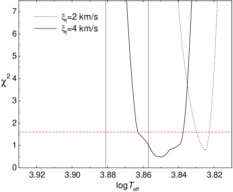
Figure 3: Behaviour of $\chi^{2}(T_{\rm eff})$ from the fits of pulsation amplitudes and phases for the dominant peak, $\nu_{1}$, which was identified as $\ell=1$. Atmospheric models were calculated with [m/H]=0.0 and two indicated values of the microturbulence velocity, $\xi_{\rm t}$. The horizontal line at $\chi^{2}=1.6$ corresponds to 80 % confidence level. The vertical lines marks the range of $T_{\rm eff}$ from mean colours.

The basic stellar parameters adopted for the present investigation were derived from the mean photometric indices and the Hipparcos parallax using NEMO.2003 models. We arrived at the following values, $\log T_{\rm eff}=3.869\pm 0.012$, $\log L/L_{\odot}=1.170\pm 0.055$. For the evaluation of the effective gravity we derived masses from our evolutionary tracks.

We should stress that also a satisfactory agreement between mean colours and pulsational data may be achieved at similar [m/H] and $\xi_{\rm t}$ with Kurucz’s models calculated without overshooting in the atmosphere.

The radiative flux derivatives needed for our method were determined by numerical differentiation of the tabular data from NEMO.2003 models. The limb-darkening coefficients were taken from Barban et al. (2003).

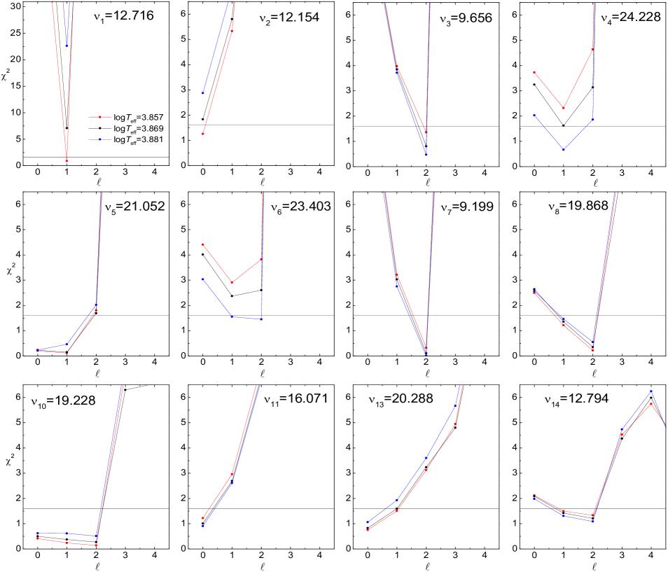
Figure 4: The values of $\chi^{2}$ as a function of $\ell$ for twelve dominant peaks in the oscillation spectrum. The assumed parameters for the atmosphere models are: $\log g=4.0$, [m/H]=0.0, $\xi_{\rm t}=4$ km s^-1, the three values of $\log T_{\rm eff}$ are given in the legend. The horizontal line at $\chi^{2}=1.6$ corresponds to the 80 % confidence level.

Table 1. Possible identification of $\ell$ (with 80 % probability) within the accepted $T_{\rm eff}$ range

$\nu$ [c/d]	our identification	Viskum et al.	Breger et al.
	from phot.&spec.	(1998)	(1999)
$\nu_{1}$= 12.716	$\ell=1$	$\ell=1$	$\ell=1$
$\nu_{2}$= 12.154	$\ell=0$	$\ell=0$	$\ell=0$
$\nu_{3}$= 9.656	$\ell=2$	$\ell=2$	$\ell=1,2$
$\nu_{4}$= 24.228	$\ell=1$	$\ell=1$	$\ell=1,2$
$\nu_{5}$= 21.052	$\ell=1,0$	$\ell=2$	$\ell=2$
$\nu_{6}$= 23.403	$\ell=2,1$	$\ell=0$	$\ell=0,1$
$\nu_{7}$= 9.199	$\ell=2$	$\ell=2$	$\ell=2$
$\nu_{8}$= 19.868	$\ell=2,1$	$\ell=2$	$\ell=2$
$\nu_{10}$= 19.228	$\ell=2,1,0$	$-$	$-$
$\nu_{11}$= 16.071	$\ell=0$	$-$	$-$
$\nu_{13}$= 20.288	$\ell=0,1$	$-$	$-$
$\nu_{14}$= 12.794	$\ell=2,1$	$-$	$-$

3.3 Identification of spherical harmonic degrees

We applied the method described in Sect. 3.1 to the twelve dominant modes in FG Vir pulsation. For all of them, we have both photometric and spectroscopic data. We use only observations made in 2002 because radial velocity measurements are only from 2002. In the present application the radial velocity data are essential because we have data only for two photometric passbands and three is the minimum if we want to rely on the pure photometric version of our method.

In Fig. 4 we plot $\chi^{2}$ as a function of $\ell$. With the adopted 80  % confidence level, corresponding to $\chi^{2}=1.6$, a unique $\ell$ identification is not always possible. The $\chi^{2}$ minima for the dominant peak and the majority of the remaining ones favour the lowest values of $\log T_{\rm eff}$ in the allowed range. There are two exceptions, the $\nu_{4}$ and $\nu_{6}$ peaks, which prefer the highest $\log T_{\rm eff}$. Of course there is only one effective temperature and we believe that it is close to $\log T_{\rm eff}\approx 3.86$, because the $\nu_{1}$ is the dominant mode and its amplitudes and phases are most accurate.

In Table 1 we compare our new $\ell$ identification with earlier attempts. The agreement is very good. We accepted only the $\ell$ values leading to $\chi^{2}\leq 1.6$, which results in a 80 % probability of the correct identification. With this criterion we could assign unique $\ell$ values to the six frequencies.

It is significant that $\ell\geq 3$ is excluded in all twelve cases at a safe confidence level. We know very little about nonlinear development of multimode instability. If only the disc averaging effect were responsible for mode selection then there would be a fair chance for detecting modes with $\ell\geq 3$. It would be so because, in the range of observed frequencies, the amplitude reduction between $\ell=1$ and $\ell=4$, for instance, is only about six, whereas all modes from $\nu_{2}$ to $\nu_{14}$ have amplitudes by factor 5 to 20 lower than the $\nu_{1}$ mode.

The identification of the $\nu_{2}$ and $\nu_{11}$ peaks as radial modes looks firm and promising. The probability that one of the modes has $\ell>0$ is less than 5 %. The frequency ratio of 0.756 is not far from the expected ratio between the fundamental mode and the first overtone. A closer look, however, reveals that achieving a close match is not easy. The corresponding model values range from 0.773 to 0.779 depending which opacity data are used in the stellar model. The lower value is obtained with the OPAL (Iglesias & Rogers 1996) and the higher one with the OP data (Seaton & Badnell 2004, Badnell et al. 2005, Seaton 2005). It seems very difficult to reconcile the ratio with models ignoring effects of rotation. As Daszyńska-Daszkiewicz et al. (2002) have shown, rotation couples the even $\ell$ modes and it is possible that for instance $\ell=4$ mode may mimic a radial mode. It is beyond the scope of the present paper to examine this possibility, but we plan to do it in the future.

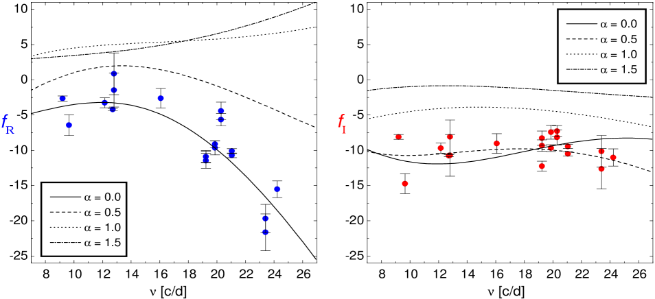
Figure 5: Comparison of the empirical values of $f$ (dots with error bars) with the theoretical ones calculated for four values of the MLT parameter, $\alpha$, adopting convective flux freezing approximation. The real and imaginary part of $f$ are shown in the left and the right panels, respectively.

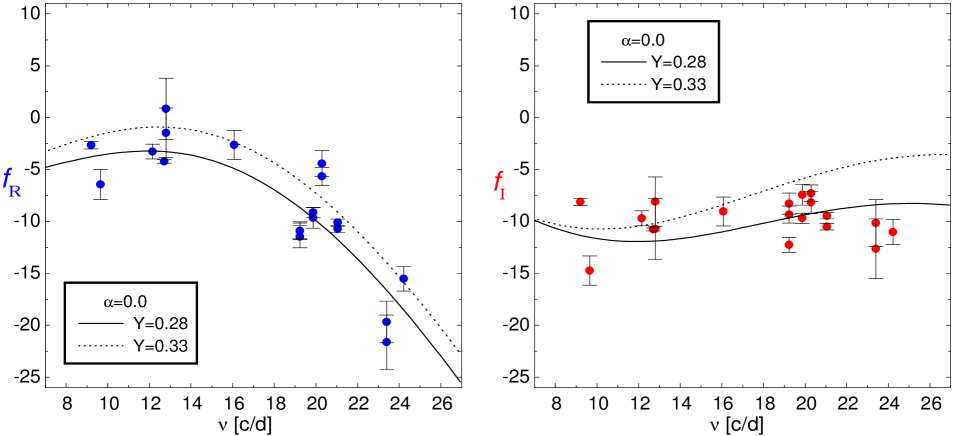
Figure 6: Comparison of the empirical values of $f$ (dots with error bars) with the theoretical ones calculated for $\alpha=0.0$ and two values of the helium abundance: $Y=0.28$ and $Y=0.33$.

4 Constraints on stellar convection

It has been shown in Paper I that calculated values of $f$ are very sensitive to how convection transport is included. Thus, a comparison with the corresponding empirical values provides a test of the adopted description of convection.

4.1 A simplistic approach

Here, as in Paper I, we begin with the same naive, but commonly adopted approach i.e. the standard mixing-length theory (MLT) and the convective flux freezing approximation. FG Vir is a relatively hot $\delta$ Sct star and, unless the MLT parameter is unrealistically large, there are two unconnected convective layers, one associated with H and the other with HeII ionization zone. The adopted approximation is indeed very bad only in the H ionization zone, where convective transport may dominate. In Fig. 5, we compare empirical values of $f$ with those calculated upon above approximations. The empirical $f$’s depend only weakly on adopted values of $T_{\rm eff}$ and $L$. The plotted values were obtained adopting $M=1.85M_{\odot}$, $\log T_{\rm eff}=3.860$ and $\log L=1.170$. These parameters are consistent with mean photometric data for FG Vir and evolutionary models, and they lead to $\chi^{2}<1.6$ as obtained with our method for most of the peaks. The empirical $f$’s are relatively insensitive also to the choice of $\ell$ which in some cases is ambiguous. For the plot, we use $\ell$’s corresponding to $\chi^{2}$ minima. The calculated $f$’s are even less $\ell$-dependent.

We can see that there is a good agreement between the empirical and the theoretical values for the models calculated with $\alpha=0.0$. This is pleasing because our approximations are irrelevant in the limit of totally inefficient convection. Calculated $f$’s shown in Fig. 5 were obtained with the OPAL opacities (Iglesias & Rogers 1996) assuming the standard Population I composition ($Y=0.28,Z=0.02$). We found that results remain essentially unchanged with the OP opacities (Seaton & Badnell 2004, Badnell et al. 2005, Seaton 2005). Also a different value of metal abundance, $Z$, has only a minimal effect. Only the change in helium abundance seems to matter a little, as it is shown in Fig. 6.

We found that our standard models calculated with $\alpha=0.0$ predict instability of all modes considered in this paper. We take it as a support for a low value of the MLT parameter and for the adopted effective temperature. However, in the complete oscillation spectrum of FG Vir there are peaks extending up to nearly 45 c/d (Breger et al. 2005). These small amplitude peaks with frequencies above 25 c/d cannot be explained in terms of unstable low-degree modes. Above 25 c/d, we found only instability of high-degree ($\ell>60$) f-modes. However, to explain the observed amplitudes in terms of such modes, we would have to postulate their large intrinsic amplitudes ($\epsilon$) implying relative temperature fluctuations $>1$, locally in the hydrogen ionization zone. Therefore, it is unlikely that such modes may explain the high frequency peaks in FG Vir. More likely, these peaks arise from the second order effect of lower frequency modes leading to peaks at harmonic or combination frequencies in the oscillation spectrum. The original modes might not be detected as peaks in the power spectrum if the aspect angle is close to the node of the spherical harmonic.

4.2 A more advanced approach

As an alternative to the simplistic models in Sect. 4.1, we considered more advanced models which estimate the turbulent fluxes by means of a nonlocal time-dependent generalization of the mixing-length formulation by Gough (1977a, 1977b). In this formulation there are two more parameters, $a$ and $b$, which control respectively the spatial coherence of the ensemble of eddies contributing to the turbulent fluxes of heat, $F_{\rm c}$, and momentum (also known as turbulent pressure), $p_{\rm t}$, and the degree to which the turbulent fluxes are coupled to the local stratification. Roughly speaking, the latter two parameters control the degree of “nonlocality” of convection: low values imply highly nonlocal solutions, and in the limit $a,b\rightarrow\infty$ the system of equations formally reduces to the local formulation (except near the boundaries of the convection zone, where the local equations are singular). Further computational details are described by Balmforth (1992) and Houdek et al. (1999).

Results presented in Fig. 7 are for different values of the mixing-length parameter $\alpha$ but for fixed $a^{2}=900$ and $b^{2}=2000$. From models computed with different values for $a$ and $b$ we concluded that the $f$ values are rather insensitive to the choice of $a$ and $b$. For the remaining convection parameters that are included in a mixing-length formulation (e.g. anisotropy parameter, see Gough, 1977b) we assumed values that are consistent with the formulation by Böhm-Vitense (1958). In the local limit ($a,b\rightarrow\infty$) and for $p_{\rm t}=0$ we obtained for the stellar models approximately the same depth of the convection zone at constant $\alpha$ between the two formulations of Sect. 4.1 and Sect. 4.2. The differences in the fractional convective heat flux between the two convection formulations, depicted in Fig. 8 for different values of $\alpha$, are predominantly a result of the effects of “nonlocality” and turbulent pressure $p_{\rm t}$.

Let us summarize the differences between the codes used to obtain the results presented in Sect. 4.1 (Fig. 5) and in Sect. 4.2 (Fig. 7). In the former case the nonlocal effects of convection and turbulent pressure were neglected in constructing the envelope models. There is also a difference in the low-temperature opacities. In the former case the Alexander & Ferguson (1994) and in the latter the Kurucz (1992) opacities were employed. Moreover, the code that was used to produce the results in Fig. 7 assumed the generalized Eddington approximation to radiative transfer, whereas the diffusion approximation was assumed in producing the results in Fig. 5.

In the pulsation calculations that lead to the $f$ values, Gough’s treatment (Fig. 7) included the perturbations of the convective heat flux and that of the turbulent pressure, both of which have been neglected in Sect. 4.1.

In spite of these differences both cases favour a small mixing-length parameter ($\alpha\la 0.5$), though the models of Sect. 4.2 (Fig. 7), which include convection dynamics, are in reasonable agreement for a broader range of $\alpha$ values ($0.25\la\alpha\la 1.0$). The large differences in $f$ between the $\alpha=0$ and $\alpha=1$ case depicted in Fig. 5 must predominantly result from the convective flux freezing approximation.

As for mode instability, the results obtained with both convection formulations are very similar. The advanced approach, which includes convection dynamics, finds unstable modes for frequencies up to about 25 c/d (i.e. up to the fifth radial mode) and for models with $\alpha$ values between 0.25 and 1.5. A similar limiting frequency value of about 25 c/d is found with the simplistic approach and with $\alpha\simeq 0$. A significantly larger range of unstable modes is predicted, up to a frequency of about 31.5 c/d, for models with $\alpha=1$. Such a large value for $\alpha$ is, however, excluded with the simplistic approach (see Fig. 5).

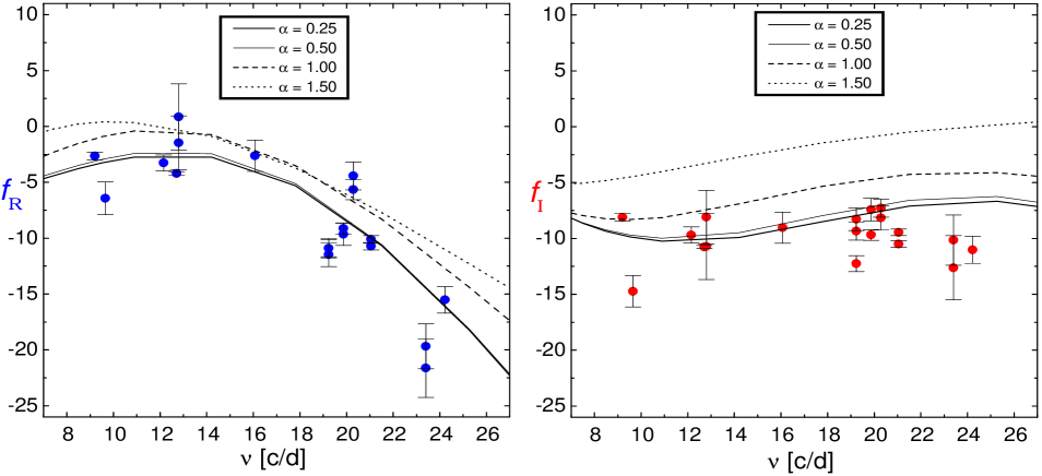
Figure 7: Similar as Fig. 5 but the theoretical values of $f$ were obtained from models using a nonlocal, time-dependent formulation of the mixing-length theory (Gough 1977a, 1977b).

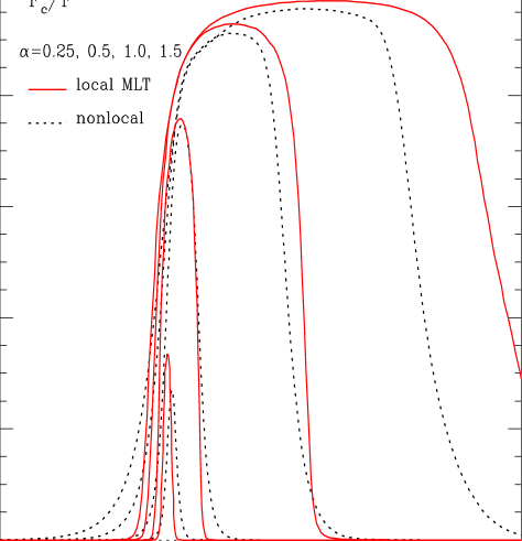
Figure 8: Comparison of the fractional heat flux carried by convection for various values of the mixing-length parameter, $\alpha$, in the standard and in the Gough’s nonlocal, time-dependent convection formalisms. Results are plotted against total pressure $P$. The maxima of $F_{\rm c}/F$ are approximately at the centre of the hydrogen ionization zones.

5 Conclusions

Using simultaneous photometric and spectroscopic data on twelve modes excited in FG Vir, we determined their spherical harmonic degrees, $\ell$, and complex parameters $f$, which link the surface flux variation to the displacement. In six cases, the $\ell$ identification is unique at the 80 % confidence level. In all twelve cases, modes with degree $\ell\geq 3$ are excluded at a very high confidence level.

The fit of the pulsation data imposes a stringent constraint on atmospheric parameters, like the effective temperature, $T_{\rm eff}$, microturbulence velocity, $\xi_{\rm t}$, and metallicity, [m/H]. From the data of the dominant peak in the oscillation spectrum, we inferred that $T_{\rm eff}$ should be close to the cooler end of the allowed range defined by the mean colours. For the microturbulent velocity we found $\xi_{\rm t}\approx 4$ km s^-1 if [m/H]$\approx 0.0$ was assumed. In the case of low amplitude modes, more accurate observations and measurements in more passbands are needed for constraining the atmospheric parameters.

Two of the uniquely identified modes are radial. However, if effects of rotation are ignored, the observed period ratio is in conflict with calculated values in standard stellar models consistent with mean parameters. We see the best chances for resolving the discrepancy by taking into account effects of rotational mode coupling. We will explore this possibility in the future.

We compared $f$ values inferred from data of twelve pulsation modes of FG Vir with theoretical values from nondadiabatic pulsation calculations which assumed various models for convection. The twelve modes cover a broad range of frequencies. We found good agreement over the whole frequency range with models for which convection dynamics was neglected and for which inefficient convection $(\alpha\simeq 0)$ was assumed. If, however, convection dynamics is included in the model calculations the results are in reasonable agreement with the data also for larger values of $\alpha$, though they are still substantially smaller than for a calibrated solar model.

- (1) Alexander, D. R., Ferguson, J. W., 1994, ApJ 437, 879
- (2) Badnell, N. R., Bautista, M. A., Butler, K., et al., 2005, MNRAS, in press (astro-ph/0410744)
- Balmforth (1992) Balmforth, N. J., 1992, MNRAS, 255,639
- Boehm-Vitense (1958) Böhm-Vitense, E., 1958, Zs. f. Ap., 46, 108
- Barban, C., Goupil, M. J., et al (2003) Barban, C., Goupil, M. J., Van’t Veer-Menneret, C. et al., 2003, A&A 405, 1095
- Breger et al. (1995) Breger, M., Handler, G., Nather, R. E. et al., 1995, A&A 297, 473
- Breger & al (1999) Breger, M., Pamyatnykh, A.A., Pikall, H., Garrido, R., 1999, A&A 341, 151
- Breger & al (2004) Breger, M., Rodler, F., Pretorius, M. L., Martín-Ruiz, S. et al., 2004, A&A 419, 695
- Breger & al (2005) Breger, M., Lenz, P., Antoci, V. et al., 2005, A&A, in press
- (10) Daszyńska-Daszkiewicz, J., Dziembowski, W. A., Pamyatnykh, A. A., Goupil, M-J. 2002, A&A 392, 151
- Daszyńska-Daszkiewicz & al (2003) Daszyńska-Daszkiewicz J., Dziembowski W.A., Pamyatnykh A.A., 2003, A&A 407, 999 Paper I
- Daszyńska-Daszkiewicz & al (2004) Daszyńska-Daszkiewicz, J., Dziembowski, W. A., Pamyatnykh, A.A., 2004, IAU Colloquium 193: Variable Stars in the Local Group, New Zealand, July 2003, eds. D. W. Kurtz & K. R. Pollard, ASP Conf. Ser., Vol. 310, p. 255
- Daszyńska-Daszkiewicz & al (2004) Daszyńska-Daszkiewicz, J., Dziembowski, W. A., Pamyatnykh, A.A., Breger M., Zima W., 2004, Cambridge University Press, eds. J. Zverko, J. Z̆iz̆nowský, S. J. Adelman & W. W. Weiss, IAUS224: The A-Star Puzzle, pp. 853-859
- Gough (1977a) Gough, D. O., 1977a, in ”Problems of Stellar Convection”, eds. E. Spiegel & J.-P. Zahn, Lecture Notes in Physics, Vol. 71, p. 15
- Gough (1977b) Gough, D. O., 1977b, ApJ, 214, 196
- Guzik (1995) Guzik, J. A., Bradley, P. A., 1995, BaltA, 4, 442
- Houdek (1999) Houdek, G., Balmforth, N. J., Christensen-Dalsgaard, J., Gough, D. O., 1999, A&A 351, 582
- Iglesias (1996) Iglesias, C. A., Rogers, F. J., 1996, ApJ, 464, 943
- Kurucz (1998) Kurucz, R. L., 1998, http://kurucz.harvard.edu
- Kurucz (1992) Kurucz, R. L., 1992, Rev. Mex. Astron. Astrofis. 23, 45
- Mittermayer (2003) Mittermayer P., Weiss W. W., 2003, A&A 407, 1097
- Nendwich (2004) Nendwich, J., Heiter, U., Kupka, F., Nesvacil, N., Weiss W. W., 2004, Comm. in Asteroseismology 144, 43
- Viskum at al (1998) Viskum, M., Kjeldsen, H., Bedding, T. R. et al. 1998, A&A 335, 549
- (24) Seaton, M. J., 2005, MNRAS, in press, (astro-ph/0411010)
- (25) Seaton, M. J., Badnell, N. R., 2004, MNRAS 354, 457
- Templeton et al (2001) Templeton, M., Basu, S., Demarque, P., 2001, ApJ 563, 999