High-Resolution Molecular Line Observations of the Environment of the Class 0 Source B1-IRS

Abstract

In this work we present VLA observations of the NH₃, CCS, and H₂O maser emission at 1 cm from the star forming region B1-IRS (catalog ) (IRAS 03301+3057 (catalog )) with $\simeq 5"$ (=1750 AU) of angular resolution. CCS emission is distributed in three clumps around the central source. These clumps exhibit a velocity gradient from red- to blueshifted velocities toward B1-IRS, probably due to an interaction with the outflow from an embedded protostar. The outflow and its powering source are traced by a reflection nebula and an associated infrared point source detected in a 2MASS K-band image. We find that this infrared point source is associated with water maser emission distributed in an elongated structure ($\simeq$ 450 AU size) along the major axis of the reflection nebula and tracing the base of the outflow of the region. Ammonia emission is extended and spatially anticorrelated with CCS. This is the first time that this kind of anticorrelation is observed in a star forming region with such a high angular resolution, and illustrates the importance of time-dependent chemistry on small spatial scales. The relatively large abundance of CCS with respect to ammonia, compared with other star forming regions, suggests an extreme youth for the B1-IRS object ($\leq$ 10⁵ yr). We suggest the possibility that CCS abundance is enhanced via shock-induced chemistry.

1 Introduction

The spatial distribution of emission from various molecular tracers in star forming clouds depends not only on the physical conditions within the clouds but also on the (time-dependent) chemistry. This is very clearly the case for CCS and NH₃, where a pronounced spatial anticorrelation in the emission from these two species has been reported for quiescent, starless cores (Suzuki et al., 1992). A spatial anticorrelation has also been observed on large scale maps in several individual sources, such as TMC-1 (catalog ) (Hirahara et al., 1992), L1498 (catalog ) (Kuiper, Langer, & Velusamy 1996), and B68 (catalog ) (Lai et al., 2003).

The lines of CCS are very appropriate for studying the structure and the physical conditions in dark clouds because they are not very opaque (Saito et al., 1987), and yet they are intense and abundant (Suzuki et al., 1992). Its lack of hyperfine splitting and the fact that it is heavier than other high-density tracers (thus showing intrinsically narrower lines) make CCS a very well-suited molecule for carrying out dynamical studies. NH₃ emission tends to trace the inner, denser regions of molecular cores, while CCS shows up slightly outside these central regions with a clumpy distribution (Suzuki et al., 1992). This relative distribution has been explained in terms of chemical and dynamical evolution of the protostellar core: CCS lines are intense in cold quiescent cores, but when the cloud evolves and star formation begins, high velocity outflows and radiation from protostars destroy carbon chain molecules. At the same time, these conditions favor the desorption of NH₃ from dust grains. For this reason, the abundance ratio [CCS]/[NH₃] has been considered as an indicator of evolution in protostellar cores (Suzuki et al., 1992).

CCS is rarely found to be associated with evolved star-forming regions. On the other hand, emission from both CCS and NH₃ has been detected from the Class 0 protostar B335 (catalog ) (Menten, Krügel, & Walmsley 1983; Velusamy, Kuiper, & Langer 1995) suggesting that a combination of both molecules can be used as a means of identifying the youngest protostars, and of studying their environments over a range of physical and chemical regimes. Class 0 protostars have been proposed to be in the earliest stages of low-mass stellar evolution (André, Ward-Thompson, & Barsony 1993). Processes related to mass-loss phenomena occur prominently during this phase: collimated jets, powerful molecular outflows, and protoplanetary disks of hundreds of AU are commonly detected in this kind of source (Chandler & Sargent, 1993; Terebey, Chandler, & André, 1993). CCS and NH₃ may therefore trace the interaction of these phenomena with the surrounding environment, providing information about the kinematics, temperature, and density in the close vicinity of very young stellar objects (YSOs).

Water maser emission has also been shown to be a good tracer of mass-loss activity in YSOs (Rodríguez et al., 1980; De Buizer et al., 2005). Previous studies suggest that water maser emission provides a good characterization of the age of low-mass YSOs, with Class 0 sources being the most probable candidates to harbor water masers (Furuya et al., 2001). Water masers have been detected in both circumstellar disks and outflows. This dichotomy has also been suggested to be a time-dependent effect, with masers tracing disks in younger objects and tracing outflows in somewhat more evolved sources (Torrelles et al., 2002).

The far-infrared source B1-IRS (IRAS 03301+3057) is one of the few sources known to exhibit both CCS and water maser emission in the studies by Suzuki et al. (1992) and Furuya et al. (2001). This is a Class 0 source (Hirano et al., 1997) located in the Perseus OB2 complex at a distance of 350 pc (Bachiller, Menten, & del Rio Álvarez 1990). The B1 (catalog ) cloud contains a large amount of molecular gas, as shown by the strong C¹⁸O(1–0) emission detected by Bachiller & Cernicharo (1984). There is no optically visible counterpart of B1-IRS, but 850 micron dust continuum emission has been detected by Matthews & Wilson (2002) using SCUBA. There are two compact SiO clumps in the vicinity of B1-IRS (Yamamoto et al., 1992), and blueshifted CO(1–0) emission observed by Hirano et al. (1997), who suggested the presence of a pole-on molecular outflow. The SiO clumps are located at the interface between the CO outflow and the dense gas traced by the C¹⁸O, suggesting that the outflow, probably driven by the IRAS source, is interacting with the surrounding medium, thus yielding the SiO emission through shocks.

In this work, we have used the Very Large Array (VLA) of the National Radio Astronomy Observatory to study the properties of the CCS, NH₃, and water maser emission from B1-IRS, in order to obtain information about its circumstellar dynamics and stage of evolution. The rest frequencies of the CCS and H₂O transitions are sufficiently close together that they can be observed simultaneously with the VLA, also offering the possibility of using the water masers to track tropospheric phase fluctuations, if the masers are strong enough. Unfortunately this was not the case at the time of the observations presented here, but the atmosphere was in any case very stable.

This paper is structured as follows: in §2 we describe our observations and data reduction procedure, as well as the analysis of VLA archive data. In §3 we present our observational results (morphology and physical parameters), which are then discussed in §4. We summarize our conclusions in §5.

2 Observations and data processing

Simultaneous observations of the J_N=2₁-1₀ transition of CCS (rest frequency $=$ 22344.033 MHz) and the 6₁₆-5₂₃ transition of H₂O (rest frequency = 22235.080 MHz) were carried out on 2003 April 4 using the VLA in its D configuration. The phase center of these observations was R.A.(J2000) = 03^h33^m16$\fs$3, Dec(J2000) = 31$\arcdeg$07$\arcmin$51$\arcsec$. We used the four IF spectral line mode, with two IFs for each molecular transition, one in each of right and left circular polarizations. For the CCS observations we sampled 128 channels over a bandwidth of 0.781 MHz centered at $V_{\rm LSR}=6.8$ km s^-1, with a velocity resolution of 0.082 km s^-1. Water maser observations were obtained using 64 channels over a 3.125 MHz bandwidth centered at $V_{\rm LSR}=15.7$ km s^-1, with 0.66 km s^-1 velocity resolution. The total on-source integration time was $\simeq$ 7.5 hours. Our primary calibrator was 3C48, for which we adopted a flux density of 1.1253 Jy (at the CCS frequency) and 1.1315 Jy (at the H₂O frequency) using the latest VLA values (1999.2). The source 3C84 was used as phase and bandpass calibrator (bootstrapped flux density = 11.80$\pm$0.14 Jy at the CCS frequency and 11.65$\pm$0.14 Jy at the H₂O frequency). Calibration and data reduction were performed with the Astronomical Image Processing System (AIPS) of NRAO.

CCS data were reduced applying spectral Hanning smoothing and natural weighting of the visibilities, to improve the signal-to-noise ratio. The final velocity resolution is 0.16 km s^-1 and the synthesized beam is 4$\farcs$33 $\times$ 3$\farcs$30 (P.A = $-$79$\fdg$2). Water maser maps were produced using a “robust” weighting (Briggs, 1995) of 0, to optimize a combination of both angular resolution and sensitivity. The synthesized beam obtained is 3$\farcs$29 $\times$ 2$\farcs$73 (P.A = 87$\fdg$9).

In order to compare our water maser results with those at other epochs, we also retrieved earlier H₂O data from the VLA archive. These observations were carried out on 1998 October 24 and 1999 February 26, in CnB and CD configuration respectively, for project AF354. These data have been published by Furuya et al. (2003). Both sets of observations were made in the 1IF spectral line mode, in right circular polarization only, with a bandwidth of 3.125 MHz centered at $V_{\rm LSR}=0$ km s^-1, and sampled over 128 channels, thus providing a velocity resolution of 0.33 km s^-1. The phase center of these observations was R.A.(J2000) = 03^h33^m16$\fs$030, Dec(J2000) = 31$\arcdeg$07$\arcmin$34$\farcs$05. The time on source was $\simeq$ 3 minutes in 1998 and $\simeq$ 13 minutes in 1999. In both epochs 3C48 was used as primary flux calibrator, with an assumed flux density of 1.1313 Jy and 1.1315 Jy for the 1998 and 1999 observations respectively (adopting the latest 1999.2 VLA values). The secondary calibrator was 0333+321, with a bootstrapped flux density of 1.66$\pm$0.10 Jy for the 1998 observations and 1.67$\pm$0.03 Jy for the 1999 observations. The water masers were strong enough during these earlier observations to enable self-calibration, after referencing the maser positions to 0333+321. Images were made with the robust parameter set to 0, giving synthesized beams of $0\farcs 91\times 0\farcs 38$ (P.A. = 81$\fdg$7) and $3\farcs 05\times 1\farcs 16$ (P.A. = 68$\fdg$8) for the 1998 and 1999 data respectively.

We have also processed VLA archive data of the NH₃(1,1) inversion transition (rest frequency = 23694.496 MHz). The observations were made on 1988 August 13 for project AG265, in the D configuration. The total bandwidth was 3.125 MHz, centered at $V_{\rm LSR}=6.1$ km s^-1 and sampled by 128 channels, which provided a velocity resolution of 0.33 km s^-1. Both right and left circular polarizations were obtained. The phase center of these observations was R.A.(J2000) = 03^h33^m16$\fs$337, Dec(J2000) = 31$\arcdeg$07$\arcmin$51$\farcs$03. The total time on source was $\simeq$ 2 h. The source 3C48 was used as the primary flux calibrator, with an adopted flux density of 1.0542 Jy (1999.2 values). The phase calibrator was 3C84 (bootstrapped flux density = 38.0$\pm$1.5 Jy). Since the NH₃ emission was faint and extended, we reduced the data using natural weights and a uv-taper of 20 k${\lambda}$, to improve the sensitivity to the extended emission. The resulting synthesized beam is $8\farcs 62\times 7\farcs 76$ (P.A. = $-75\fdg 5$). The size of the VLA primary beam at the frequencies corresponding to the CCS, H₂O and NH₃ transitions ($\simeq$22 GHz) is $\simeq$ 2$\arcmin$.

To have an estimate of the missing flux density due to the lack of short spacings of the VLA, we have obtained single-dish spectra of both CCS and NH₃ towards the position R.A.(J2000) = 03^h33^m16$\fs$3, Dec(J2000) = 31$\arcdeg$07$\arcmin$51$\arcsec$, with the NASA’s 70 m antenna (DSS-63) at Robledo de Chavela, Spain, at the same frequencies as the VLA. This antenna has a 1.3 cm receiver comprising a cooled high-electron-mobility transistor (HEMT) amplifier. A noise diode is used to calibrate the data. The half power beam width at this frequency is $\simeq$ 41^′′, and the mean beam efficiency is $\simeq$ 0.4. Observations were made in frequency switching mode, using a 256 channel autocorrelator spectrometer. The CCS observations were performed in six time slots between 2002 August and 2003 July with a total integration time of 60 minutes and an average system temperature of $\simeq$ 80 K. We used a bandwidth of 1 MHz (velocity resolution = 0.05 km s^-1). The NH₃ observations were carried out during 2003 July, with an average system temperature of $\simeq$ 60 K. The on-source integration time was 40 minutes. To detect all the hyperfine lines we used a bandwidth of 10 MHz (velocity resolution = 0.5 km s^-1). The rms pointing accuracy of the telescope was better than 9^′′. All the single-dish data reduction was carried out using the CLASS package, developed at IRAM and the Observatoire de Grenoble as part of the GAG software.

In addition to the radio data, we have retrieved a K-band image from the Two Micron All Sky Survey (2MASS), to obtain a better position for the infrared source. This image was smoothed with a 5$\arcsec$ Gaussian (FWHM), to search for low surface-brightness, extended emission.

3 Results

3.1 The infrared source

The 2-$\micron$ map obtained from the 2MASS archive, and convolved with a 5$\arcsec$ Gaussian (Fig. 1), shows a point source, designated 2MASS J03331667+3107548 (catalog ), at R.A.(J2000) = 03^h33^m16$\fs$678, Dec(J2000) = 31$\arcdeg$07$\arcmin$54$\farcs$88 (2$\sigma$ absolute position error $\simeq 0\farcs$22). This position is $\simeq 6\arcsec$ away from the IRAS catalog position, R.A.(J2000) = 03^h33^m16$\fs$3, Dec(J2000) = 31$\arcdeg$07$\arcmin$51$\arcsec$, but well within the error ellipsoid (2$\sigma$ error axes = 48$\arcsec$$\times$14$\arcsec$) of the latter. In what follows, we will consider the position of the 2MASS point source as the location of the central source of B1-IRS. We also find extended 2 $\mu$m infrared emission elongated to the south west of the point source, with position angle $\simeq-120\arcdeg$, suggestive of a reflection nebula.

3.2 The water masers

Our water maser observation on April 2003 shows a cluster of 23 maser spots (Table 1), spatially unresolved in each channel, most of which are redshifted with respect to the cloud velocity ($V_{\rm LSR}=6.3$ km s^-1; Hirano et al. 1997) with LSR velocities between 9.1 and 23.6 km s^-1, although three are blueshifted, with LSR velocities between 2.5 and 3.8 km s^-1. The maximum flux density was $\simeq$ 15.4$\pm$1.6 mJy at $V_{\rm LSR}$ = 17.7 km s^-1, two orders of magnitude weaker than in the earlier epochs reported by Furuya et al. (2003). The masers are distributed in an elongated structure (P.A. $\simeq-120\arcdeg$), with a length of $\simeq$ $1$$\farcs$$3$ ($\simeq$455 AU).

We have compared our new data with those obtained in 1998 October and 1999 February by Furuya et al. (2003). The maser positions for those epochs are shown in Fig. 2, and in Tables 2 and 3. The same elongated distribution is evident. In these earlier data sets all maser emission is redshifted with respect to the cloud velocity. We note that there is a discrepancy of $\simeq$23$\arcsec$ between the positions of the 1998 October masers presented here and the positions reported in Table 3 of Furuya et al. (2003) using the same data. The positions of the masers (that we have determined by fitting two-dimensional Gaussians to the maser spots detected in each channel), are similar in all three epochs, taking into account their mean absolute positional uncertainties ($\simeq$ 0$\farcs$3, 0$\farcs$16, and 0$\farcs$04 for 2003 April, 1999 February and 1998 October respectively). Therefore we are confident that our positions are correct.

The water masers are located at a distance $\lesssim$ 1$\arcsec$ (350 AU) from the 2$\micron$ source, suggesting that this is the center of activity of the region. Considering an average LSR velocity of $\simeq$ 14.0 km s^-1 of the maser emission, i.e., $\simeq$ 7.7 km s^-1 redshifted with respect to the cloud velocity (6.3 km s^-1), and a mean distance of $0\hbox to0.0pt{.\hss}^{\prime\prime}5$ from the central source, the central mass needed for the water masers to be gravitationally bound is $\simeq 12$ M_☉. However, B1-IRS is a low luminosity protostar ($L\simeq 2.8$ L_☉, Hirano et al. 1997), and it is unlikely to be much more massive than $\simeq 1$ M_⊙. These results strongly suggest that the masers are tracing mass loss motions rather than bound motions in a circumstellar disk.

3.3 CCS and NH₃ emission

3.3.1 CCS emission

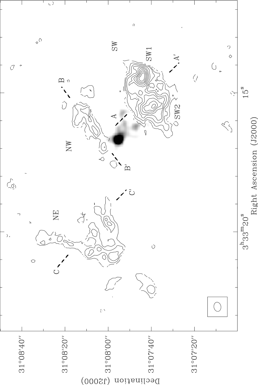
Figure 3: CCS integrated emission (contours) not corrected for the response of the VLA primary beam, overlaid on the 2MASS K-band emission (grey scale). Contour levels range from 0.66 to 5.94 mJy beam^-1 km s^-1 in intervals of 0.66 mJy beam^-1 km s^-1. Grey scale ranges between 10% and 45% of the peak emission (the source magnitude is K = 14.208$\pm$0.122 measured by 2MASS). The south-west (SW), north-west (NW) and north-east (NE) CCS clumps are labeled. Dashed lines represent the axes where position-velocity diagrams have been obtained (Fig. 6) .

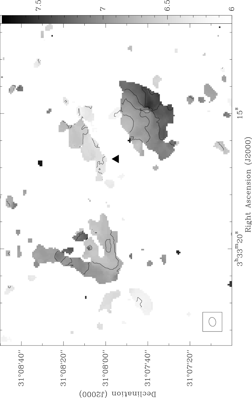
Figure 5: Map of CCS intensity-weighted mean velocity (first-order moment). Contour levels range from 6.0 to 7.8 km s^-1 at steps of 0.2 km s^-1. The grayscale is also from 6.0 to 7.8 km s^-1. The filled triangle represents the position of the 2 $\mu$m source.

The integrated emission from the CCS molecule is distributed in three clumps (Fig. 3). The clump centers are located $\simeq$ 25$\arcsec$ (9000 AU) south-west (SW clump), $\simeq$ 50$\arcsec$ (17000 AU) north-east (NE clump), and $\simeq$ 15$\arcsec$ (5000 AU) north-west (NW clump) from the central source. Fig. 4 shows the CCS emission integrated over different velocity intervals. All clumps are redshifted with respect to the systemic velocity of the B1 core ($V_{\rm LSR}$ = 6.3 km s^-1). Moreover, the SW, NE and NW CCS clumps show clear velocity gradients of $\simeq$ 23, $\simeq$ 10, and $\simeq$ 12 km s^-1 pc^-1 respectively (see Figs. 5 and 6) over the whole size of the clumps, with velocities closer to that of the ambient cloud near the central object.

Clump SW has the most redshifted velocities ($V_{\rm LSR}$ from 6.6 km s^-1 to 7.6 km s^-1). It has an ellipsoidal shape, elongated perpendicularly to the direction of the velocity gradient, with two emission peaks. Clump NE shows emission from $V_{\rm LSR}$ = 6.6 km s^-1 to 7.1 km s^-1, and it is divided into three “fingers” that point towards the north-west. Clump NW has a velocity gradient from $V_{\rm LSR}$ = 6.3 to 6.8 km s^-1 (i.e., closer to the mean cloud velocity), and its morphology is elongated, with its major axis pointing towards the central source.

3.3.2 NH₃ emission

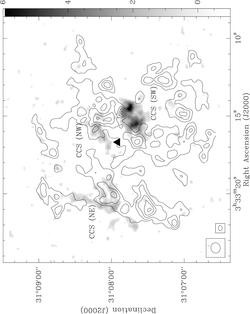
Figure 7: CCS (greyscale) and ammonia main line (contours) integrated emission. Greyscale ranges from -1 to 6 mJy beam^-1 km s^-1. Contour levels range from 40 to 120 mJy beam^-1 km s^-1 with increment steps of 20 mJy beam^-1 km s^-1 , the rms of the map. Filled triangle represents the 2 $\mu$m source. The beam on the left correspond to the ammonia observations and the beam on the right corresponds to the CCS observations. No primary beam correction has been applied to these maps. However, given that the phase center was almost the same in the CCS and NH₃ observations, the beam response is similar and does not affect the comparison between both emissions.

Ammonia emission is very extended and clumpy (Fig. 7). Most clumps are distributed in two strips, with NW-SE orientation. The general trend, however, as illustrated by Fig. 7, is that CCS and NH₃ emissions are spatially anticorrelated. Such an anticorrelation has been observed in other sources (Hirahara et al., 1992; Willacy, Langer, & Velusamy, 1998; Lai et al., 2003), but this is the first time that it has been detected with such a high angular resolution ($\simeq$ 5$\arcsec$).

We have to note, however, that there is considerable extended NH₃(1,1) and CCS (J_N=2₁-1₀) emission in the B1-IRS region to which the VLA is not sensitive. Indeed, from our single-dish observations of these transitions (Fig. 8) we estimate that $\simeq$ 90% of the ammonia and CCS emission is missed with the VLA.

3.3.3 Physical parameters

Although the maps shown in this paper have not been corrected by the primary beam response for display proposes, such a correction has been applied to the data prior to deriving physical parameters. Table 4 summarizes the main physical parameters obtained from the CCS and NH₃ lines. For the CCS data, we provide parameters for each individual clump, since they are well defined in the integrated intensity map (Fig. 3). For these calculations, we have divided the emission of the SW clump in two different peaks, SW1 (located at lower right ascension), and SW2 (located at the eastern part of the SW clump). The mean clump column density of CCS is $N_{\rm CCS}\simeq(3.0\pm 0.8)\times 10^{13}$cm^-2, which is similar to the value obtained by Suzuki et al. (1992) for B1 ($1.38\times 10^{13}$ cm^-2). Assuming a relative abundance of CCS with respect to H₂ of $0.9\times 10^{-10}$ (mean value reported by Lai & Crutcher 2000 for B1), the resulting mean $N_{\rm H_{2}}$ is $\simeq(3.3\pm 0.8)\times 10^{23}$ cm^-2.

Given the low signal-to-noise ratio and the clumpy structure of the NH₃ emission, we only give averaged values for this molecule in Table 4. The column density of ammonia at each local maximum seen in the integrated intensity map (Fig. 7), ranges between $\simeq 6\times 10^{14}$ and $3\times 10^{15}$ cm^-2, with a mean clump value of $\simeq(1.4\pm 0.4)\times 10^{15}$ cm^-2 , similar to the value of $1\times 10^{15}$ cm^-2 reported by Bachiller & Cernicharo (1986).

4 Discussion

4.1 The geometry of the molecular outflow

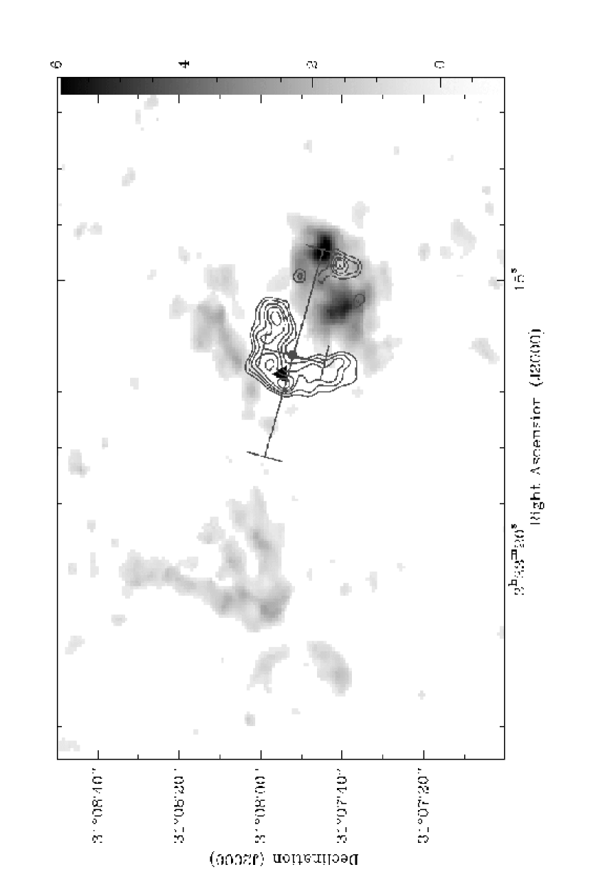
Figure 9: Overlay of the CO blueshifted outflow (contours; Hirano et al. 1997) and CCS integrated emission (greyscale; this paper). The filled circle represents the IRAS source with its error position barrs. The triangle marks the 2 micron point source. The CCS emission is not corrected from the response of the primary beam.

Hirano et al. (1997) detected moderately-high velocity blueshifted CO emission centered close to the position of the IRAS source and consisting of many clumps at different blueshifted velocities. No redshifted emission was obvious in their data. Given the distribution of the blueshifted gas around the IRAS position (Fig. 9), Hirano et al. (1997) suggested the existence of a molecular outflow driven by the IRAS source, and oriented pole-on with respect to the observer. In order to explain the absence of the redshifted CO lobe, these authors suggested that higher density material is slowing down that component of the outflow.

Our results, however, do not support the pole-on geometry for the outflow. The 2MASS source, which is within the error box of the IRAS position, is located at the tip of the blueshifted outflow, rather than at its center (see Fig. 9). If we assume that the 2MASS source is actually tracing the powering source of the outflow (confirmed by its association with the water masers), its blueshifted lobe would flow towards the southwest from the central source.

The low velocity of the CO blueshifted emission with respect to the $V_{\rm LSR}$ of the cloud ($|V_{\rm CO}-V_{\rm LSR}|<$ 8 km s^-1), and the lack of a significant amount of redshifted gas, are more compatible with the molecular outflow being close to the plane of the sky. The absence of a coherent velocity gradient of the water masers along their linear structure is also consistent with this geometry.

4.2 The outflow traced by water masers

The water masers are distributed in the direction of the extended infrared nebula, approximately NE-SW. This is the same orientation as the blueshifted CO lobe with respect to the central source, and suggests that the masers are tracing the base of the outflow. Note, however, that most of the maser components are redshifted with respect to the cloud velocity, and yet their location primarily to the south and west of the infrared source means that they coincide with the blueshifted CO lobe. This apparent kinematic discrepancy could be explained if the masers are tracing the background walls of a cavity evacuated in the cloud by a molecular outflow close to the plane of the sky. The existence of such a cavity was suggested by Hirano et al. (1997) form their C¹⁸O map. In the proposed geometry of an outflow close to the plane of the sky, the background walls could show redshifted motions, assuming a finite opening angle. The fact that no corresponding blueshifted masers are shown tracing the foreground walls could be due to different physical conditions of the gas, with denser gas in the background (that probably corresponds to the region that goes deeper into the molecular cloud), and would produce a stronger interaction with the outflow in that area. Proper motion measurements of the B1-IRS water masers will help to clarify wether our proposed geometry, with the outflow close to the plane of the sky and evacuating a cavity in the cloud, is correct.

4.3 The interaction between the molecular outflow and its surrounding environment

The CCS clumps show a clear velocity gradient, with less redshifted velocities towards the central source (see Fig. 5). If we assume that the ambient cloud velocity is 6.3 km s^-1 (Hirano et al., 1997), these clumps would be redshifted with respect to the cloud velocity. This velocity pattern cannot be explained purely by foreground clumps with infalling motions, for which we would expect more redshifted velocities closer to the source. Nevertheless, if we consider that the CCS clumps may be interacting with the outflowing material, the infalling clumps could be slowed down closer to the central source due to this interaction, explaining in this way the less redshifted velocities at these positions.

An alternative scenario to explain the CCS kinematics is outflowing clumps driven by a wind. If this wind exhibits a Hubble-flow type velocity, that increases with distance from the driving source (as it is observed in other outflows from class 0 protostars, Chandler & Richer 2001), we could explain the velocity pattern by background clumps interacting with, and being accelerated by the outflowing material. In order to have redshifted CCS emission at both to the NE and SW from the central source, the outflow must lie near the plane of the sky, and the CCS clumps should be associated with the back side of the outflow, both for the southwestern blueshifted CO lobe, and the (as yet) undetected northeastern redshifted CO lobe.

A way to distinguish between these two models (foreground infalling clumps decelerated by the outflow vs. background outflowing accelerated clumps), is to ascertain whether the motions observed in the CCS clumps can be gravitationally bound.

There are two main components in the observed motions: the internal velocity gradients within the clumps, and the bulk velocity of the whole clump with respect to the central source. For the first component, the mass M needed to gravitationally bind a cloud of size $R$ with velocity gradient $dV/dl$ is $M=V^{2}RG^{-1}$, with $V=(dV/dl)R$. This means that the masses needed to bind the internal gradient within each clump are 1.3, 0.3, and 0.4 $M_{\sun}$ for clumps SW, NW, and NE, respectively.

The masses derived for the clumps (Table 4) are of the same order of those necessary for the clumps to be bound, although we must consider this result carefully due to the very large uncertainties involved in these calculations.

On the other hand, if we consider an average velocity of each CCS clump with respect to that of the ambient cloud, and the distance from the infrared source to the center of each clump, the masses needed to bind the motions respectively for SW, NW, and NE CCS clumps as a whole are 6, 0.4, and 6 $M_{\sun}$ respectively. The mass of gas contained in a region of radius equal to the distance to the central source would be 13-30 $M_{\sun}$ for the SW clump, 5-11 $M_{\sun}$ for the NW clump, and 51-120 $M_{\sun}$ for the NE clump, depending on the values of $N_{H_{2}}$ obtained from either averaged values for NH₃ or CCS.

Therefore, we see that the observed motions in the CCS clumps can be gravitationally bound, a fact that does not allow us to discard either of the alternative models. Regardless of the real geometry and dynamics of the region, it seems that there is an important interaction of the ambient gas with the molecular outflow.

We must point out that the observed CCS clumps may not really be physical entities. These clumps are likely to represent regions of enhanced abundance of CCS (Suzuki et al., 1992; Ohashi et al., 1999). This chemical gradient of CCS is a result of variations in the local conditions of the cloud (Lai et al., 2003). However, our mass estimates to check if the motions are gravitationally bound are still valid even if the enhanced CCS emission are not physical clumps, given that we are calculating the mass of the region of gas enclosed by the CCS emission. The largest source of uncertainty is the value of the molecular abundance, which is a common problem when deriving column densities using other molecular tracers. In our calculations we consider a fractional abundance of CCS with respect to the H₂ of 0.9$\times$10^-10, that is the mean value reported by Lai & Crutcher (2000) for this region.

4.4 Chemical evolution: CCS vs. NH₃

Single-dish observations show that the CCS is more abundant in starless, cold, quiescent dark cores (such as L1521B (catalog ), L1498 (catalog ), TMC-1C (catalog ) or L1544 (catalog ); Suzuki et al. 1992) while ammonia emission tends to be intense in star-forming regions. These results suggested that CCS is a tracer of early time chemistry (t $\leq$ 10⁵ yr), while ammonia is a tracer of more evolved gas (Hirahara et al., 1992; Velusamy et al., 1995; Bergin & Langer, 1997).

The abundance ratio $N_{\rm NH_{3}}/N_{\rm CCS}$ has therefore been proposed by Suzuki et al. (1992) as an indicator of the evolutionary stage of molecular clouds. Our single dish data provides column densities of $N_{\rm NH_{3}}\simeq(6\pm 4)\times 10^{14}$ and $N_{\rm CCS}\simeq(1.70\pm 0.24)\times 10^{13}$ cm^-2. Thus, the ratio $N_{\rm NH_{3}}/N_{\rm CCS}$ is $\simeq$35, which is significantly lower than the value $\geq 100$ found by Suzuki et al. (1992) in most of the star forming regions in their survey. This relative lack of ammonia, or enhanced CCS, may be an indication of the early evolutionary stage of B1-IRS. However this result could depend on the particular chemistry of each region, and we must be careful in this interpretation.

In previous single-dish works, a spatial anticorrelation between CCS and ammonia was found, both by comparing detections of those molecules in surveys of sources (Suzuki et al., 1992), and by mapping their emission in the same region (Lai et al., 2003). It is interesting to check whether this anticorrelation still stands when we map a source at high resolution. The overlay of our CCS and ammonia maps (Fig. 7) shows a clear anticorrelation between them throughout the B1-IRS region, except $\simeq 30^{\prime\prime}$ to the north of the ammonia maximum (which coincides with the NE CCS clump), where there is some superposition. This is the first time that this anticorrelation is observed at such a high-resolution ($\simeq 5^{\prime\prime}$ = 1750 AU) in a star-forming region, and illustrates that the chemistry is not only time-dependent, but also exhibits small-scale spatial structure that can potentially seriously affect the interpretation of derived physical and dynamical properties if it is not properly taken into account.

The chemical gradients traced by these molecules may be the result of changing the local conditions. At this moment, most of the theoretical chemical models considering the age and distance to the cloud center, include a large number of physical parameters to study the variation of the column density, the distribution, and the fractional abundance of molecules like CCS and NH₃ among other species. Some of these models include the strength of magnetic fields, initial chemical composition of the cloud, the probability of molecules sticking to dust grains, cosmic-ray ionization rate, and cloud mass (Shematovich et al., 2003), UV photodisociation, cosmic-ray induced photoionization and photodisociation reactions, CO depletion onto grains, and desorption by cosmic-rays (Nejad & Wagenblast, 1999), or core geometry and view angles (Aikawa, Ohashi, & Herbst, 2003). Until now, these chemical studies focused on starless cores and did not consider the effects of a central star, probably because most of the CCS studies have been made toward starless cores (Kuiper et al., 1996; Ohashi et al., 1999; Lai et al., 2003; Shinnaga et al., 2004).

The way in which all of these factors and the activity of protostars (in the case of star forming regions) can modify the classical ion-molecule or radical/neutral pathways of production of molecules like CCS (Smith, 1988; Suzuki et al., 1988; Petrie, 1996; Scappini & Codella, 1996) needs to be studied in theoretical works to give a better interpretation of our results. The development of models that implement the onset of energetic activity associated with the formation of a star and how this affects the CCS and NH₃ production will be the key to ascertain the evolutionary stage of B1-IRS. Models treating consistently both CCS and NH₃ and considering the effect of young stars could provide more reliable values of the relative abundances and column densities of both molecules as a function of the distance from the source. On the other hand, our data on B1-IRS could be used as a reference work to test the predictions of those calculations in detail. Future comparison with other regions observed with high angular resolution will be vital for understanding the precise meaning of the ratio between CCS and NH₃ abundances in star-forming regions, in terms of chemical evolution.

Moreover, detailed chemistry studies in molecular clouds are an important science driver for the development of new interferometers (e.g. SMA or ALMA, see van Dishoeck & Blake 1998; Phillips & Vastel 2003). Our anticorrelation result at small scale proves that chemistry studies is indeed a promising line of research for these new telescopes.

The clumpy distribution of CCS emission detected in B1-IRS, has already been observed by other authors in several molecular clouds such as B335 (catalog ) (Velusamy et al., 1995), L1498 (catalog ) (Kuiper et al., 1996), and TMC-1 (catalog ) (Langer et al., 1995). In the case of B1-IRS, this clumpy distribution was first detected by Lai & Crutcher (2000) in the CCS J_N= 3₂-2₁ transition at 33.8 GHz with the BIMA interferometer with an angular resolution of $\simeq$ 30^′′. In particular, there seems to be a spatial coincidence between BIMA clumps F and B and our VLA clumps SW and NE respectively. Moreover our VLA observations reveal a lack of CCS emission at the position of B1-IRS. This absence of emission has been suggested to be due to a lower abundance of the molecule, rather than to a density decrease, since this molecule needs high density to be excited and the density is expected to be higher towards the center (Velusamy et al., 1995). The clumpy distribution could be due to an episodic infall (as suggested by Velusamy et al. 1995 for B335).

Another possibility that it is worth considering is that CCS might be locally enhanced in shocked regions. In fact, the observed CCS clumps show kinematical signs of interaction with the outflow, which suggests that the CCS emission could be originated from gas affected by the impact of shocks. The outflow could squeeze low density gas to the higher densities ($\simeq$ 10⁵ cm^-3) needed to produce the CCS, and trigger the formation of the molecule. Such low density gas exists around dense clouds like B1, and the outflow associated to B1-IRS could interact with fresh material around the dense core. Although there is currently no chemical model that includes this kind of phenomena related to the star formation, to support the suggested enhancement, observations of other molecules have suggested that their abundance is enhanced in the environment of jets and outflows, by shock-induced chemistry, as in the case of CS (Arce & Sargent, 2004), NH₃ (Torrelles et al., 1992, 1993), or HCO⁺ (Girart et al., 2000). Theoretical chemistry models support those findings (Taylor & Williams, 1996; Viti, Natarajan, & Williams, 2002; Wolfire & Koenigl, 1993). In particular, for HCO⁺ it has been proposed that in some cases its abundance may be increased by a fast outflow impinging on fragments of dense gas (Rawlings, Taylor, & Williams, 2000), and this type of interaction between outflow and dense gas is also suggested by our CCS data, although the chemical reactions involved will certainly be different.

If this abundance enhancement takes place in short timescales ($\simeq$ 10⁵ yr), one could expect to find clumps of the order of 5^′′ at the distance of B1 (350 pc), considering a typical sound speed of $\simeq$ 0.1 km s^-1. Therefore, new interferometric observations of CCS in other star-forming regions would be necessary to study these processes.

The association of the central source with water maser emission (which typically lasts for $\simeq$ 10⁵ yr in star forming regions; Forster & Caswell 1989) and the existence of CCS, a molecule characteristic of early time chemistry (Hirahara et al., 1992; Suzuki et al., 1992) confirm the early stage of evolution of B1-IRS. The presence of CCS can be used as a marker of extreme youth among Class 0 protostars (de Gregorio-Monsalvo 2005, in preparation). Furthermore, this combination of spatial, kinematic, and dynamical information from the CCS and ammonia may be used as a powerful tool to study the processes taking place in the vicinity of very young Class 0 protostars and not just in quiescent cores.

Clearly, further interferometric CCS observations of the environment of other young stellar objects as well as theoretical chemistry models will be useful to determine whether CCS emission tends to selectively trace regions of interaction of the outflow with its surrounding medium. These studies combined with high-resolution data of NH₃ and other molecular tracers will also help to determine the spacial distribution and dinamical evolution of these species.

5 Conclusions

We have presented high resolution observations of ammonia, CCS, and water masers toward the Class 0 object B1-IRS (IRAS 03301+3057). Our main conclusions are as follows:

• There is a 2MASS infrared point source located $\sim 6\arcsec$ NE from the nominal position of the IRAS source, and at the NE tip of a blueshifted CO outflow lobe. Fainter infrared emission extending towards the SW from the point source is also detected.

• There is a group of water masers associated with the infrared point source. Their elongated distribution (in the NE-SW direction), and their unbound motions suggest that these masers are tracing the base of the outflow.

• The infrared and water maser data suggest that the infrared point source traces the position of the powering source of the mass-loss phenomena in the region, and that mass is ejected along the NE-SW direction.

• We detect three clumps of CCS emission surrounding the infrared source, all redshifted with respect to the systemic cloud velocity. They show clear velocity gradients, with less redshifted gas towards the central source. We interpret these gradients in terms of clumps that are strongly interacting with a molecular outflow that lies almost in the plane of the sky.

• Ammonia emission is weak and extended. It shows a spatial anticorrelation with CCS. Although this kind of anticorrelation is known to be present in other star-forming regions, this is the first time that it has been observed with such a high-angular resolution ($\simeq 5^{\prime\prime}$).

• The abundance ratio between ammonia and CCS is significantly lower than that found in other star-forming regions. Given the fast disappearance of CCS in star-forming regions, this low ratio might be an indication of B1-IRS being an extremely young stellar object ($\leq$ 10⁵ yr).

• We suggest the possibility that CCS abundance is enhanced via shock-induced chemistry. However, theoretical calculations will be needed to confirm this hypothesis.

Figure 1: 2MASS K-band image convolved with a 5$\arcsec$ Gaussian. Contours represent 90%, 75%, 60%, 45%, 30%, and 15% of the peak emission (the source magnitude is K = 14.208$\pm$0.122, measured by 2MASS). Crosses and open circles in the close-up of the infrared emission (right panel) represent the structure of red and blueshifted water masers respectivelly, obtained in the April 2003 observations and scaled by their relative position uncertainty.

Figure 2: Positions of water masers observed towards B1-IRS at different epochs. Open pentagons, filled squares, and crosses represent the maser components observed in October 1998, February 1999, and April 2003, respectively. The position offsets are relative to the 2 micron point source, which is represented by a filled triangle. The northernmost maser spot shown in Fig. 1 is out of the scale in this plot.

Figure 4: Contour maps of the CCS integrated emission over the LSR velocity ranges (in km s^-1) indicated in the top right corner of each panel. Contour levels are at $-2.56$, $-1.92$, and from $1.92$ to $7.68$ at steps of 0.64 mJy beam^-1 km s^-1 (the rms of the maps). Filled triangle indicates the 2 $\mu$m point source position. No primary beam correction has been applied to these figures.

Figure 6: Position-velocity diagrams of the CCS clumps. The upper panel represents the position-velocity diagram of the NW clump through axis B-B’ (see Fig. 3), the central one corresponds to the NE clump through axis C-C’, and the bottom one the SW clump through axis A-A’. Contours are at $-3.6$, and from $3.6$ to $9.6$ mJy beam^-1 with steps of 1.2 mJy beam^-1, the rms of the maps. These plots have not been corrected from the response of the VLA primary beam.

Figure 8: Single-dish spectra observed with the Robledo 70m antenna, at the position R.A.(J2000) = 03^h33^m16$\fs$34, Dec(J2000) = 31$\arcdeg$07$\arcmin$51$\farcs$1. Left panel represents the NH₃(1,1) emission, with rms noise $1\sigma=0.08$ K. Right panel is the CCS(2₁-1₀) spectrum, with rms noise $1\sigma=0.13$ K.

Table 1: Water maser components on 2003 April 04

Right Ascension	Declination	Position	Flux density	$V_{\rm LSR}$
(J2000)	(J2000)	uncertainty ($\arcsec$)	(mJy)	(km s-1)
03 33 16.62	31 07 54.6	0.3	4.3$\pm$1.6	9.1
03 33 16.629	31 07 54.89	0.17	7.3$\pm$1.7	3.8
03 33 16.63	31 07 54.3	0.3	4.9$\pm$1.7	19.0
03 33 16.63	31 07 54.6	0.3	3.9$\pm$1.7	22.3
03 33 16.636	31 07 54.58	0.17	7.1$\pm$1.7	10.4
03 33 16.64	31 07 54.3	0.4	3.2$\pm$1.7	22.9
03 33 16.641	31 07 54.88	0.13	9.7$\pm$1.6	14.4
03 33 16.643	31 07 54.98	0.13	9.3$\pm$1.6	11.7
03 33 16.648	31 07 55.06	0.09	13.1$\pm$1.6	15.0
03 33 16.650	31 07 54.89	0.14	8.6$\pm$1.6	18.3
03 33 16.65	31 07 54.9	0.3	4.7$\pm$1.7	16.4
03 33 16.656	31 07 54.88	0.09	14.7$\pm$1.7	12.4
03 33 16.657	31 07 55.01	0.08	15.4$\pm$1.6	17.7
03 33 16.659	31 07 55.02	0.16	7.8$\pm$1.7	3.2
03 33 16.659	31 07 55.17	0.19	6.4$\pm$1.6	11.1
03 33 16.665	31 07 55.09	0.17	6.9$\pm$1.6	9.8
03 33 16.666	31 07 55.15	0.12	10.6$\pm$1.6	13.7
03 33 16.670	31 07 54.99	0.10	12.3$\pm$1.7	13.1
03 33 16.67	31 07 55.2	0.3	3.6$\pm$1.7	2.5
03 33 16.68	31 07 56.3	0.3	4.0$\pm$1.6	23.6
03 33 16.684	31 07 54.92	0.12	7.1$\pm$1.7	17.0
03 33 16.684	31 07 55.02	0.13	9.2$\pm$1.6	15.7
03 33 16.70	31 07 55.1	0.3	4.1$\pm$1.6	19.7

Table 2: Water maser components on 1998 October 24

Right Ascension	Declination	Position	Flux density	$V_{\rm LSR}$
(J2000)	(J2000)	uncertainty ($\arcsec$)	(mJy)	(km s-1)
03 33 16.6493	31 07 55.049	0.024	440$\pm$80	15.1
03 33 16.6498	31 07 55.039	0.020	570$\pm$90	14.8
03 33 16.6504	31 07 55.080	0.017	750$\pm$100	14.5
03 33 16.6509	31 07 55.061	0.019	560$\pm$80	14.2
03 33 16.651	31 07 55.10	0.03	610$\pm$90	13.8
03 33 16.6538	31 07 55.062	0.009	2300$\pm$300	16.1
03 33 16.654	31 07 55.04	0.03	360$\pm$70	13.5
03 33 16.6591	31 07 55.067	$\cdots$	2800$\pm$300	15.8
03 33 16.6593	31 07 55.069	0.011	970$\pm$130	15.5
03 33 16.661	31 07 55.06	0.15	1050$\pm$140	16.5
03 33 16.667	31 07 55.11	0.07	130$\pm$60	16.8

Table 3: Water maser components on 1999 February 25

Right Ascension	Declination	Position	Flux density	$V_{\rm LSR}$
(J2000)	(J2000)	uncertainty ($\arcsec$)	(mJy)	(km s-1)
03 33 16.591	31 07 54.91	0.16	137$\pm$23	19.1
03 33 16.628	31 07 54.69	0.14	118$\pm$20	12.8
03 33 16.636	31 07 55.11	0.25	57$\pm$27	20.1
03 33 16.641	31 07 54.95	0.04	352$\pm$24	15.1
03 33 16.641	31 07 54.96	0.04	362$\pm$21	13.2
03 33 16.646	31 07 55.00	0.05	36$\pm$30	17.4
03 33 16.646	31 07 55.07	0.13	142$\pm$22	18.1
03 33 16.6465	31 07 55.017	0.014	1180$\pm$50	17.1
03 33 16.647	31 07 55.02	0.16	152$\pm$23	18.4
03 33 16.6470	31 07 55.006	$\cdots$	6500$\pm$230	15.8
03 33 16.6481	31 07 55.021	0.003	6010$\pm$220	16.1
03 33 16.6481	31 07 55.026	0.007	2090$\pm$80	15.5
03 33 16.6483	31 07 55.013	0.006	2810$\pm$100	16.5
03 33 16.649	31 07 54.99	0.04	410$\pm$30	13.5
03 33 16.649	31 07 55.03	0.06	236$\pm$23	13.8
03 33 16.6493	31 07 55.017	0.008	1810$\pm$70	16.8
03 33 16.65	31 07 55.1	0.3	45$\pm$24	19.8
03 33 16.653	31 07 54.95	0.17	98$\pm$23	17.8
03 33 16.660	31 07 55.04	0.10	169$\pm$23	14.2
03 33 16.66	31 07 55.3	0.4	27$\pm$20	11.2
03 33 16.663	31 07 55.08	0.13	17$\pm$30	19.4
03 33 16.663	31 07 55.20	0.14	111$\pm$22	18.8
03 33 16.666	31 07 54.87	0.11	108$\pm$21	14.8
03 33 16.684	31 07 54.95	0.14	104$\pm$20	14.5

Table 4: Physical parameters of the clumps observed in NH₃ and CCS

Molecule	Clump	Iν	$\int{I_{\nu}dv}$	$N_{\rm mol}$	$N_{\rm H_{2}}$	Sizes	$M_{c}$
		(mJy beam-1)	(mJy beam-1 km s-1)	($10^{13}$ cm-2)	($10^{23}$ cm-2)	(AU$\times$ AU)	($M_{\sun}$)
NH3	Mean	170$\pm$30	210$\pm$30	140$\pm$40	1.4$\pm$0.4	10700$\times$4600	2.1$\pm$0.6
CCS	SW1	14.2$\pm$2.8	7.5$\pm$1.4	3.7$\pm$1.7	4.1$\pm$1.9	2900$\times$2900	1.1$\pm$0.5
CCS	SW2	10.5$\pm$2.8	6.0$\pm$1.4	2.9$\pm$1.5	3.2$\pm$1.7	5000$\times$2900	1.4$\pm$0.7
CCS	NW	4.7$\pm$2.6	3.4$\pm$1.3	1.7$\pm$1.1	1.9$\pm$1.2	7000$\times$2100	0.8$\pm$0.5
CCS	NE	9.3$\pm$3.9	7.3$\pm$2.0	3.6$\pm$1.7	4.0$\pm$1.9	12600$\times$2900	4.4$\pm$2.0

References

- Aikawa, Ohashi, & Herbst (2003) Aikawa, Y., Ohashi, N., & Herbst, E. 2003, ApJ, 593, 906
- André et al. (1993) André, P., Ward-Thompson, D., & Barsony, M. 1993, ApJ, 406, 122
- Arce & Sargent (2004) Arce, H. G. & Sargent, A. I. 2004, ApJ, 612, 342
- Bachiller & Cernicharo (1984) Bachiller, R. & Cernicharo, J. 1984, A&A, 140, 414
- Bachiller & Cernicharo (1986) Bachiller, R. & Cernicharo, J. 1986, A&A, 166, 283
- Bachiller et al. (1990) Bachiller, R., Menten, K. M., & del Río Álvarez, S. 1990, A&A, 236, 461
- Bergin & Langer (1997) Bergin, E. A. & Langer, W. D. 1997, ApJ, 486, 316
- Briggs (1995) Briggs, D. 1995, Ph.D. thesis, New Mexico Inst. of Mining and Technology
- Chandler & Sargent (1993) Chandler, C. J. & Sargent, A. I. 1993, ApJ, 414, L29
- Chandler & Richer (2001) Chandler, C. J. & Richer, J. S. 2001, ApJ, 555, 139
- De Buizer et al. (2005) De Buizer, J. M., Radomski, J. T., Telesco, C. M., & Piña, R. K. 2005, ApJS, 156, 179
- Forster & Caswell (1989) Forster, J. R. & Caswell, J. L. 1989, A&A, 213, 339
- Furuya et al. (2001) Furuya, R. S., Kitamura, Y., Wootten, H. A., Claussen, M. J., & Kawabe, R. 2001, ApJ, 559, L143
- Furuya et al. (2003) Furuya, R. S., Kitamura, Y., Wootten, A., Claussen, M. J., & Kawabe, R. 2003, ApJS, 144, 71
- Girart et al. (2000) Girart, J. M., Estalella, R., Ho, P. T. P., & Rudolph, A. L. 2000, ApJ, 539, 763
- Herbst & Klemperer (1973) Herbst, E. & Klemperer, W., 1973, ApJ, 185, 505
- Hirahara et al. (1992) Hirahara, Y., Suzuki, H., Yamamoto, S., Kawaguchi, K., Kaifu, N., Ohishi, M., Takano, S., Ishikawa, S., Masuda, A. 1992, ApJ, 394, 539
- Hirano et al. (1997) Hirano, N., Kameya, O., Mikami, H., Saito, S., Umemoto, T., & Yamamoto, S. 1997, ApJ, 478, 631
- Ho & Townes (1983) Ho, P. T. P. & Townes, C. H. 1983, ARA&A, 21, 239
- Kuiper et al. (1996) Kuiper, T. B. H., Langer, W. D., & Velusamy, T. 1996, ApJ, 468, 761
- Lai et al. (2003) Lai, S., Velusamy, T., Langer, W. D., & Kuiper, T. B. H. 2003, AJ, 126, 311
- Lai & Crutcher (2000) Lai, S. & Crutcher, R. M. 2000, ApJS, 128, 271
- Langer et al. (1995) Langer, W. D., Velusamy, T., Kuiper, T. B. H., Levin, S., Olsen, E., & Migenes, V. 1995, ApJ, 453, 293
- Matthews & Wilson (2002) Matthews, B. C. & Wilson, C. D. 2002, ApJ, 574, 822
- Menten, Krügel, & Walmsley (1983) Menten, K. M., Krügel, E., & Walmsley, C. M. 1983, Mitteilungen der Astronomischen Gesellschaft Hamburg, 60, 409
- Nejad & Wagenblast (1999) Nejad, L. A. M. & Wagenblast, R. 1999, A&A, 350, 204
- Ohashi et al. (1999) Ohashi, N., Lee, S. W., Wilner, D. J., & Hayashi, M. 1999, ApJ, 518, L41
- Petrie (1996) Petrie, S. 1996, MNRAS, 281, 666
- Phillips & Vastel (2003) Phillips, T. G., & Vastel, C. 2003, SFChem 2002: Chemistry as a Diagnostic of Star Formation, proceedings of a conference held August 21-23, 2002 at University of Waterloo, Waterloo, Ontario, Canada N2L 3G1. Edited by Charles L. Curry and Michel Fich. NRC Press, Ottawa, Canada, 2003, p. 3., 3
- Rawlings, Taylor, & Williams (2000) Rawlings, J. M. C., Taylor, S. D., & Williams, D. A. 2000, MNRAS, 313, 461
- Rodríguez et al. (1980) Rodríguez, L. F., Moran, J. M., Gottlieb, E. W., & Ho, P. T. P. 1980, ApJ, 235, 845
- Saito et al. (1987) Saito, S., Kawaguchi, K., Yamamoto, S., Ohishi, M., Suzuki, H., & Kaifu, N. 1987, ApJ, 317, L115
- Scappini & Codella (1996) Scappini, F. & Codella, C. 1996, MNRAS, 282, 587
- Shematovich et al. (2003) Shematovich, V. I., Wiebe, D. S., Shustov, B. M., & Li, Z. 2003, ApJ, 588, 894
- Shinnaga et al. (2004) Shinnaga, H., Ohashi, N., Lee, S., & Moriarty-Schieven, G. H. 2004, ApJ, 601, 962
- Smith (1988) Smith, I. W. M. 1988, ASSL Vol. 146: Rate Coefficients in Astrochemistry, 106
- Suzuki et al. (1988) Suzuki, H., Ohishi, M., Kaifu, N., Kasuga, T., Ishikawa, S., & Miyaji, T. 1988, Vistas in Astronomy, 31, 459
- Suzuki et al. (1992) Suzuki, H., Yamamoto, S., Ohishi, M., Kaifu, N., Ishikawa, S., Hirahara, Y., & Takano, S. 1992, ApJ, 392, 551
- Taylor & Williams (1996) Taylor, S. D., & Williams, D. A. 1996, MNRAS, 282, 1343
- Terebey, Chandler, & André (1993) Terebey, S., Chandler, C. J., & André, P. 1993, ApJ, 414, 759
- Torrelles et al. (1993) Torrelles, J. M., Gómez, J. F., Ho, P. T. P., Anglada, G., Rodríguez, L. F., & Cantó, J. 1993, ApJ, 417, 655
- Torrelles et al. (2002) Torrelles, J. M., Patel, N. A., Gómez, J. F., & Anglada, G. 2002, Rev. Mexicana Astron. Astrofís. Ser. Conf., 13, 108
- Torrelles et al. (1992) Torrelles, J. M., Rodríguez, L. F., Cantó, J., Anglada, G., Gómez, J. F., Curiel, S., & Ho, P. T. P. 1992, ApJ, 396, L95
- van Dishoeck & Blake (1998) van Dishoeck, E. F. & Blake, G. A. 1998, ARA&A, 36, 317
- Velusamy et al. (1995) Velusamy, T., Kuiper, T. B. H., & Langer, W. D. 1995, ApJ, 451, L75
- Viti, Natarajan, & Williams (2002) Viti, S., Natarajan, S., & Williams, D. A. 2002, MNRAS, 336, 797
- Willacy, Langer, & Velusamy (1998) Willacy, K., Langer, W. D., & Velusamy, T. 1998, ApJ, 507, L171
- Wolfire & Koenigl (1993) Wolfire, M. G., & Koenigl, A. 1993, ApJ, 415, 204
- Wolkovitch et al. (1997) Wolkovitch, D., Langer, W. D., Goldsmith, P. F., & Heyer, M. 1997, ApJ, 477, 241
- Yamamoto et al. (1992) Yamamoto, S., Mikami, H., Saito, S., Kaifu, N., Ohishi, M., & Kawaguchi, K. 1992, PASJ, 44, 459