Friedmann cosmology on codimension 2 brane with time dependent tension

Abstract

A solution of codimension 2 brane is found for which 4 dimensional Friedmann cosmology is recovered on the brane with time dependent tension, in the Einstein frame. The effective parameter $p/\rho$ of equation of state on the brane can be quintessence like, de Sitter like or phantom like, depending on integration constants of the solution.

In 1983 Rubakov and Shaposhnikov presented an extraordinary model rubakov to solve the cosmological constant problem, in which the cosmological constant appeared as an integration constant. In this model the effective cosmological constant was free of the zero point quantum energy. The zero point energy only warps the extra dimension, and at the same time our 4 large dimensional spacetime keeps flat. This is similar to the case that although in realistic universe the 4 dimensional curvature may be high but the 3 dimensional spatial curvature is almost zero.

During recent years codimension 1 brane model has been fairly well understood. Also the cosmology in frame of codimension 1 brane has been thoroughly studied, for a review see lang . Generally speaking codimension 1 cosmology of RS model implies Friedmann equation like

$$H^{2}\sim\rho+\frac{\rho^{2}}{\sigma},$$ (1)

where $\sigma$ is the brane tension, $\rho$ is the energy density of matter on the brane. We find the standard cosmology recovers when the energy scale is low enough and the corrected Friedmann equation gives notable effect when the energy scale is high enough . But to the codimension 2 case, we get into a much more weird situation: although the effective cosmological constant is independent of the tension of the brane, to our surprise, we appear to be very restricted in our permitted brane energy-momentum. Typically, a brane in its ground state has a very special energy-momentum tensor, which is isotropic and has the property that energy density=–pressure navarro , that is to say, the only spacetime allowed is maximally symmetric space, no Friedmann cosmology with generic parameter of state equation $p/\rho$ can be set up on the brane.

To circumvent this embarrassed situation and get a viable cosmology on codimension 2 brane, different authors have put much effort. Clearly, two possible ways are available. First, inspired by the early work on cosmic string gott , a fat brane is a natural way to circumvent this problem. A such model has been considered in vinet , in which a codimension 2 braneworld with spherical extra dimensions compactified by magnetic flux is studied. Assuming Einstein gravity, it shows that when the brane contains matter with an arbitrary parameter of equation of state, and find that the universe expands consistently with standard Friedmann cosmology. However, the cost is the relation between the brane tension and the bulk deficit angle becomes  $\delta\sim\rho-3p$  for a general equation of state. This relation does not imply a self-tuning of the effective 4D cosmological constant. So this progress is bankrupt in the merit that the effective cosmological constant is independent of the brane tension, which is not what we want. In navarro the action includes classical Hilbert action, we may curious whether or not a higher order Ricci scalar terms can circumvent the restriction energy density=–pressure on the brane. That is the second accessible possibility. A proposal along this direction has been presented in bost , in which a general braneworld in 6 dimensional Einstein-Gauss-Bonnet gravity is studied. It shows how the 4 dimensional Einstein equation is recovered for the induced metric and matter on the brane. It also shows that relaxing regularity of the curvature in the vicinity of the brane gives rise to an additional possible correction to the Einstein equation. Now within this proposal the 4 dimensional Einstein equation recovers on the brane, therefore the Friedmann cosmology can be obtained on the brane without question. But we may bring forward the following questions to this suggestion: why in pure classical domain we must consider higher order correction to revive Einstein equation on the brane? If the $R^{2}$ term correction gives the answer that we need, as the authors stressed, since $O(R^{2})$ corrections to the Hilbert Lagrangian do arise in the low energy limit of string theory, the inclusion of this type of term could be regarded as mandatory if one wants to embed any braneworld solution into string/M-theory, how about the more higher order corrections? They may give “false” results.

In this paper we successfully recover almost realistic Friedmann cosmology on the brane in frame 6 of dimensional Einstein gravity with a 3 brane on which the tension is variable. If the brane tension originates from the quantum zero energy, it would decay with the expansion of the universe, as suggested in schu . That article addresses the question of whether non-perturbative effects of self-interacting quantum fields in curved space-times may yield a significant contribution to the tension. Focusing on the trace anomaly of quantum chromo-dynamics (QCD), a preliminary estimate of the expected order of magnitude yields

$$\rho=nH,$$ (2)

where $n=m^{3}$, $m$ is energy scale of QCD chiral phase transition, $\rho$ is vacuum energy (brane tension) and $H$ is Hubble parameter. $H$ is defined as

$$H=\frac{1}{a}\frac{da}{dt}.$$ (3)

As a natural generalization of $Z_{2}$ symmetry in codimension 1 brane model, the metric ansatz is taken to be

$$ds^{2}=-dt^{2}+a(t)^{2}d\vec{x}^{2}+dr^{2}+b(t)^{2}v(r)^{2}d\theta^{2},$$ (4)

where $d\vec{x}^{2}$ is the metric of 3 dimensional maximally symmetric space, $v(r)=\sin(r),~{}~{}r,$  or,   $\sinh(r)$, depending on the internal space is a sphere, plane or pseudosphere. To spherical case the internal space is compact by nature. And to case of plane or pseudosphere the internal space is compactfied by proper identification, that is to say, we identify all the points $r=$constant. The brane stands at $r=0$. Supposing the metric is regular on the brane, it is easy to get the familiar result in codimension 2 infinite thin braneworld models navarro ; bost

$$1-b=4G_{6}\sigma,$$ (5)

where $\sigma$ is the brane tension which equals the energy density of the brane, and $G_{6}$ denotes the 6 dimensional Newton constant. According to Schutzhold’s investigation the brane tension is proportional to the Hubble parameter, as shown in equation (2). In its original form the coefficient is related to the energy scale of QCD chiral phase transition. Although it gives right energy scale of our observed cosmological constant, we should not restrict us to the energy scale of QCD phase transition from the theoretical view because various phase transitions may happen in the history of our universe. Here we adopt a more generic case,

$$\rho(t)=\sigma(t)=\frac{1}{4G_{6}}cH,$$ (6)

in which $c$ is a constant, it can contain all the contributions of phase transitions ever happened on the brane. Note that the dimension of $c$ is $[l]$. Thus a smaller $c$ corresponding to a higher energy scale. Einstein field equations of this system is

$${}^{(6)}G_{AB}=8\pi G_{6}T_{AB},$$ (7)

where

$$T_{AB}=T_{AB}^{(bu)}+T_{AB}^{(br)},$$ (8)

${}^{(6)}G_{AB}$ denotes 6 dimensional Einstein tensor, $T_{AB}$ is the total energy momentum tensor, $T_{AB}^{(bu)}$ and $T_{AB}^{(br)}$ represent the energy on the brane and in the bulk respectively, and $G_{6}$ is the 6 dimensional Newton constant. The brane energy momentum is shown clearly in matrix form,

$$T_{AB}^{(br)}=\left(\begin{array}[]{ccc}\hat{T}_{\mu\nu}^{(br)}\delta(r)&{}\hfil&{}\hfil\\ {}\hfil&0&{}\hfil\\ {}\hfil&{}\hfil&0\end{array}\right),$$ (9)

where $\hat{T}_{\mu\nu}^{(br)}=-\sigma(t)g_{\mu\nu}$, and $\mu$ or $\nu$ runs from 0 to 3. We do not try to specify $T_{AB}^{(bu)}$ here because we will find later that it has to take a form of non perfect fluid for a self consistent solution under condition (6). Now consider the functions $a(t)$ and $b(t)$ in the following forms

$$a(t)=c_{3}e^{\frac{2(c_{2}+t)}{c}}\cosh^{2}[\frac{(t+c_{2})\sqrt{4+2c^{2}c_{1}}}{2c}],$$ (10)

and

$$b(t)=-1-\sqrt{4+2c_{1}c^{2}}\tanh[\frac{(t+c_{2})\sqrt{4+2c^{2}c_{1}}}{2c}].$$ (11)

Here $c_{1},~{}c_{2},~{}c_{3}$ are 3 integration constants. We shall explain their physical meanings later in Einstein frame. One can verify that $a(t)$ and $b(t)$ solve the 6 dimensional Einstein equation with non perfect fluid in the bulk. We can prove it is the unique solution satisfying the following conditions:
1. The metric is spatially flat, that is, $d\vec{x}^{2}$ in (4) is Euclidean.
2. Although we permit the matter in the bulk to be non perfect fluid, we impose the condition $-{T^{(bu)}}^{0}_{0}={T^{(bu)}}^{1}_{1}={T^{(bu)}}^{2}_{2}={T^{(bu)}}^{3}_{3}$, to ensure that it behaves as perfect fluid along the brane. From the physical viewpoint it is a reasonable requirement.
Here we will present some other notes on this solution. Both $a(t)$ and $b(t)$ are internal–curvature–independent, that is, they do not depend on the Gaussian curvature of the internal space, which means, spherical, flat and pseudospherical internal spaces correspond to the same $a(t)$ in (10). The tension of the brane is time dependent, which most probably leads to the time dependence of the energy momentum tensor in the bulk. We find it is just the case. Explicitly,

$$-{T^{(bu)}}^{0}_{0}=\frac{3\cosh[f]^{-3}\left((4-c_{1}c^{2})\cosh[f]+(12+5c_{1}c^{2})\cosh[f]+2l(4+(4+\frac{l^{2}}{2}\cosh[f])\sinh[f])\right)}{16c^{2}\pi G_{6}(1+l\tanh[f])},$$ (12)

and

$${T^{(bu)}}^{4}_{4}={T^{(bu)}}^{1}_{1}+\frac{1}{16\pi G_{6}}\left(-\frac{3}{2}l^{2}\cosh[f]^{-2}+6(4+c_{1}c^{2}+2l\tanh[f])\right),$$ (13)

where $f=\frac{l(c_{2}+t)}{2c}$ and $l=\sqrt{4+2c_{1}c^{2}}$. $-{T^{(bu)}}^{0}_{0}={T^{(bu)}}^{1}_{1}={T^{(bu)}}^{2}_{2}={T^{(bu)}}^{3}_{3}$ and ${T^{(bu)}}^{4}_{4}$ are also internal–curvature–independent. The situation is different to ${T^{(bu)}}^{5}_{5}$, it is internal–curvature–dependent. To avoid complexity we only give specific form of the flat internal space case,

$${T^{(bu)}}^{5}_{5}={T^{(bu)}}^{1}_{1}+\frac{72+30c_{1}c^{2}-\frac{33l^{2}}{2}\cosh[f]^{-2}+6l+\left(6+c_{1}c^{2}-\frac{l^{2}}{2}\cosh[f]^{-2}\right)\tanh[f]}{8\pi G_{6}c^{2}(1+l\tanh[f])}.$$ (14)

To the cases of sphere and pseudosphere the discussions are similar. This model also possesses another remarkable property. There is a non zero energy flux along the $r$ direction emerging in the bulk. In the case of flat internal space, it has the form as

$$w_{4}=-{T^{(bu)}}_{40}=\frac{l^{2}\cosh[f]^{-2}}{16\pi G_{6}cr(1+l\tanh[f])}.$$ (15)

This is exactly a rational result. We see the vacuum energy of the brane is decaying, but there is nothing on the brane to absorb the energy decayed . Therefore the only way out of this energy is to flow into the bulk. There is a singularity in (15) at $r=0$, where the brane habitats. Any finite energy flux flowing from the brane must be divergent at the neighborhood of the brane , since the brane is infinite thin. In respect to these results we are able to predict the energy flux vanishes at $r=\pi$ in case of spherical internal space and slopes more sharply with respect to $r$ in case of pseudospherical internal space. In fact these are just the main differences of bulk energy fluxes between flat and spherical or pseudospherical internal spaces. Still another point deserves to address. There is a deficit angle in the extra dimension due to the existence of the brane in all previous works on the codimension 2 brane models bost ; vinet ; navarro . Here, however, from (11) it is clear the “deficit angle” is negative, or, there is a surplus angle $2\pi(|b|-1)$ since $|b|>1$. For example the internal space becomes a mandarin orange rather than an American football in case of spherical internal space.

If we believe only Einstein frame makes sense in our real world, it is not obvious whether or not the solution (10) really represents a generic Friedmann universe. Now we turn to Einstein frame, in which the metric becomes

$$ds_{E}^{2}=-|b|dt^{2}+|b|a^{2}d\vec{x}^{2}.$$ (16)

Define proper time

$$d\tau=|b|^{1/2}dt,$$ (17)

and the proper scale factor,

$$\tilde{a}=|b|^{1/2}a.$$ (18)

Define cosmic velocity

$$V_{e}=\frac{d\tilde{a}}{d\tau},$$ (19)

and cosmic acceleration

$$A_{c}=\frac{d^{2}\tilde{a}}{d\tau^{2}}.$$ (20)

Now it is time for explaining the physical meanings of the constants $c_{1},~{}c_{2},~{}c_{3}$. Obviously $c_{3}$ is only a constant scale factor, and $c_{2}$ represents a relocation of initial time in (10). To make out the meaning of $c_{1}$, we calculate the proper Hubble parameter

$$\tilde{H}=\frac{V_{e}}{\tilde{a}}.$$ (21)

We find

$$\tilde{H}(t=-c_{2})=\frac{3}{c}+\frac{c_{1}c}{2}.$$ (22)

It is clear that in some sense $c_{1}$ indicates initial cosmic velocity. Naively when $c^{2}c_{1}=-2$ this solution degenerates to a de Sitter brane without angle deficit in the bulk in view of $b=-1$. Even this most simple case is not the trivial one studied before, because in our case $\sigma$ is not a constant all the same, while $\sigma=$constant in all present studies.

The most significant parameters from the viewpoint of observations are parameter of state equation $w=\frac{\rm pressure}{\rm energy~{}density}$ and the deceleration parameter $q$ of the total cosmic fluid. The two parameters are closely related to each other. Therefore, we calculate the effective $w$ and $q$ corresponding to the proper scale factor and proper time. By definition

$$w_{\rm eff}=\frac{p_{\rm eff}}{\rho_{\rm eff}}=-\frac{V_{e}^{2}+2aA_{c}}{3V_{e}^{2}},$$ (23)

and

$$q=-\frac{aA_{c}}{V_{e}^{2}},$$ (24)

we arrive at

$$q=\frac{4c_{1}c^{2}(3+c_{1}c^{2})\cosh[f]-(10+\frac{5}{2}l^{2}+l^{4})\cosh[f]+3(4+3c_{1}c^{2}+2c_{1}c^{2}l\sinh[f]-2(3+c_{1}c^{2})l\sinh[f])}{(c_{1}-2(3+c_{1}c^{2})\cosh[f]-3l\sinh[f])^{2}u},$$ (25)

and

$$w_{\rm eff}=-\frac{1}{3}+\frac{2}{3}q,$$ (26)

where $u=\sqrt{1+l\tanh[f]}$. The equations are rather complicate. It needs some labour to check when $c^{2}c_{1}>-2$, the universe finally becomes quintessence like phase, which in some sense can simulate dark matter plus cosmological constant universe; when $c^{2}c_{1}=-2$, it is a de Sitter phase; and when $c^{2}c_{1}<-2$, the universe goes into a phantom like phase. This is our main result: Friedmann universe of rather arbitrary parameters of state equations can recover on the codimension 2 varying–tension–brane. Different types of the universe depend on different choices of the integration constants. We show this result clearly in some figures. The figures illustrate that the evolution of the universe only depends on $c^{2}c_{1}$. Recall equation (6), $c$ is the vacuum energy on the brane. It is clear we can always choose a proper $c_{1}$ to counter the effect of an arbitrarily large $c$. Accordingly the most important virtue of prior models with 2 extra dimensions rubakov ; navarro is retained in our model. One may be afraid that if $c^{2}c_{1}<-2$, the arguments of the hyperbolic functions in (25) become imaginary numbers. But we find the final results always keep real even if the imaginary arguments appear.

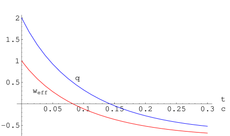
Figure 1: $\frac{t}{c}$ versus $w_{\rm eff}$ and $q$: the left part.
To showing clearly the properties of $w_{\rm eff}$ and $q$ we plot two figures with the same set of parameters, in which $t$ is in different intervals of real line. To this figure $\frac{t}{c}\in(0,0.3)$, and to the next $\frac{t}{c}\in(0.3,3)$. In this figure $c_{1}c^{2}=1$ , $c_{2}$ has been tuned such that $w_{\rm eff}=1$ when $t=0$.

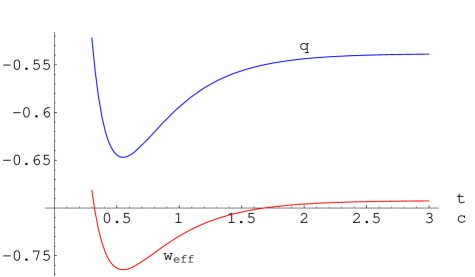
Figure 2: $\frac{t}{c}$ versus $w_{\rm eff}$ and $q$: the right part.
   In this figure the parameters are chosen as same as the last figure. These two figures show that a universe undergoes stiff matter, radiation, dust like phases and finally becomes a quintessence like universe. From the observations we know that $w_{\rm eff}$ is declining, so we may think that the current universe corresponds to the coordinate $\frac{t}{c}=0.3$. If it is true in the future $w$ will decrease for some time and then increase, eventually reach approximately –0.68.
Because the age of our universe is model dependent we can not obtain zero energy from $\frac{t}{c}=0.3$ by using the value of $t$ in the standard model. But we point out that for any given $c$ we can always obtain such a universe, as shown in figure 1 and figure 2, by tuning $c_{1}$.

Figure 3: $\frac{t}{c}$ versus $w$.
In this figure $c_{1}c^{2}=-0.5$. This figure shows that we can adopt parameters to ensure the final value of $w$ equals 0.72, which may offer some implications on the coincidence problem.

Figure 4: $\frac{t}{c}$ versus $w$.
In this figure $c_{1}c^{2}=-2.1$. A phantom dominated universe emerges under this parametrization.

To sum up: in this paper we discuss a codimension 2 braneworld model, in which the brane tension depends on time. We find a unique solution under some reasonable considerations. According to this solution Friedmann cosmologies , which permit different parameters of state equations, can be set up on the brane in Einstein frame. This is sharply different from the previous researches on this topic. At the same time our model keeps the most impressive character of the codimension 2 brane model—the effective cosmological constant is free of the absolute value of the brane tension. In our model the parameter of state equation only depends on the integration constants, that is to say, it circumvents the famous $10^{120}$ contradiction. So the problem becomes why the integration constants are taking those values.

We will also point out some questions to be discussed future in our model. Follow from figure 1, if it is believed that we are living at $t/c=0.3$, there exists another coincidence problem, which is essentially the choices of integration parameters, all the same. The asymptotic behavior of the universe in figure 3 overcomes the coincidence problem, but it is difficult to simulate the history of our universe, especially the history of structure formation. It is still an open problem in present stage.

Acknowledgments: This work was supported in part by a grant from Chinese academy of sciences, a grant No. 10325525 from NSFC, and by the ministry of science and technology of China under grant No. TG1999075401.

References

- (1) V. A. Rubakov and M. E. Shaposhnikov, Phys. Lett. B 125, 139 (1983).
- (2) D. Langlois, hep-th/0209261.
- (3) I. Navarro, JCAP, 0309 (2003), 004, hep-th/0302129; S. M. Carroll and M. M. Guica, hep-th/0302067.
- (4) J. R. Gott III, APJ, 288 (1985), 422.
- (5) J. Vinet and J. M. Cline, Phys.Rev. D70 (2004) 083514, hep-th/0406141.
- (6) J. Schwindt and C. Wetterich, hep-th/0501049.
- (7) P. Bostock, R. Gregory, I. Navarro and J. Santiago, Phys.Rev.Lett. 92 (2004), 221601, hep-th/0311074.
- (8) R. Schutzhold, Phys. Rev. Lett. 89, 081302 (2002), gr-qc/0204018.