Anti-solar differential rotation

Abstract

The differential rotation of anti-solar type detected by observations for several stars may result from a fast meridional flow. The sufficiently intensive meridional circulation may be caused by large-scale thermal inhomogeneities or, perhaps, by tidal forcing from a companion star. First results of simulations of the anti-solar rotation of a giant star with magnetically induced thermal inhomogeneities are presented. Perspectives for observational check of the theory are discussed.

1 Introduction

This paper discusses possible theoretical explanations for observations of non-uniform stellar rotation with the angular velocity increasing with latitude. It also suggests the possibilities for observational check of the theory.

The anti-solar rotation is relatively seldom to observe. The solar-like case of rotation rate decreasing with latitude is more frequent to detect (Strassmeier [2003], Petit et al. [2004]). The relatively fast rotation of the equator represents also the case which theory succeeded to explain. Theory of angular momentum transport by rotating turbulence and numerical simulations both show meridional fluxes of the angular momenrtum towards equator (Rüdiger & Hollerbach [2004]). Models for differential rotation based on that theory provide rotation law for the Sun (Kitchatinov & Rüdiger [1995], Kitchatinov [2004]) in close agreement with helioseismology (Shou et al. [1998]). Observations of solar-type rotation for AB Dor (Donati & Collier Cameron [1997]) and LQ Hya (Kovári et al. [2004]) can be reproduced with reasonable accuracy (Collier Cameron et al. [2001], Kitchatinov et al. [2000]), and theoretical trend for differential rotation of main-sequence dwarfs to decrease with spectral type (Kitchatinov & Rüdiger [1999]) was given some observational support (Collier Cameron [2001], Petit et al. [2004]).

However, observations of anti-solar rotation are already numerous enough to demand a revision of theory. The standard hydrodynamical models cannot reproduce this case. The most plausible way for such a revision is to include some additional driver of meridional flow. We shall see in the next section that the fast meridional circulation is the most clear theoretical possibility for producing differential rotation of the anti-solar type. Observations may help a lot in understanding the nature of stellar differential rotation by checking whether all the stars which show anti-solar rotation do indeed possess a fast meridional flow.

The fast meridional motion can result from a barocline driving due to large thermal spots or from tidal forcing by a close companion. The guess is suggested by both theoretical arguments and statistics of differential rotation observations for individual stars summarized by Strassmeier ([2003]). All stars with detected anti-solar rotation belong to one of two (yet small) groups: (i) close binaries, or (ii) rapidly rotating giants with large-scale thermal inhomogeneties (Hackman et al. [2001], Strassmeier et al. [2003]). The suggestion that all anti-solar rotators are spotted giants or close binaries is more speculative and less certain than the conclusion on the role of meridional flow but may also be a subject for observational verification.

After a general discussion of possible origin of anti-solar rotation in the next section, section 3 outlines a numerical model for equatorial deceleration on a giant star with large-scale thermal inhomogeneties caused by magnetic fields. Results of first simulations are presented and discussed in section 4. The final section 5 suggests the ways for observational verification of the theory.

2 General consideration

2.1 Anti-solar rotation for fast meridional flow

Possible reason for anti-solar differential rotation can be inferred from consideration of a global axisymmetric flow in a spherical convective shell. The flow velocity, $\bf u$, can be expressed in terms of the stream-function, $\psi$, of the meridional circulation and angular velocity, $\Omega$, using the standard spherical coordinates, $r,\vartheta,\varphi$,

$${\mbox{\boldmath$u$}}=\left({1\over\rho r^{2}\sin\vartheta}{\partial\psi\over\partial\vartheta},\ {-1\over\rho r\sin\vartheta}{\partial\psi\over\partial r},\ r\sin\vartheta\ \Omega\right).$$ (1)

The flow obeys the steady motion equation,

$$\rho\left({\mbox{\boldmath$u$}}\cdot\nabla\right){\mbox{\boldmath$u$}} + \left(\left({\mbox{\boldmath$B$}}\cdot\nabla\right){\mbox{\boldmath$B$}}-\nabla B^{2}/2\right)/\left(4\pi\right)$$ (2)

$$+ \nabla p-\rho\nabla\Phi=-{\rm div}\left(\rho Q\right).$$

where $B$ is magnetic field, $\Phi$ is gravity potential, and $\hat{Q}$ is the correlation tensor of fluctuating velocities, $\mbox{\boldmath$u$}^{\prime}$,

$$Q_{ij}=\langle u^{\prime}_{i}u^{\prime}_{j}\rangle.$$ (3)

The most promising for producing anti-solar rotation is a fast meridional flow. One can find that from the equation for angular velocity which results as $\phi$-component of Eq. (2),

$${1\over\sin^{2}\vartheta}\ {\partial\psi\over\partial r}\ {\partial\left(\sin^{2}\vartheta\Omega\right)\over\partial\vartheta}-{1\over r^{2}}\ {\partial\psi\over\partial\vartheta}\ {\partial\left(r^{2}\Omega\right)\over\partial r}\ \ ...=0,$$ (4)

where only the contribution of meridional flow is written explicitly. The dotted terms in (4) can be neglected if the flow is fast enough. Then, the solution can be found,

$$\Omega(r,\vartheta)={F(\psi)\over r^{2}\sin^{2}\vartheta},$$ (5)

which describes almost certainly the inhomogeneous rotation of the anti-solar type. The angular momentum is conserved along stream lines of a fast meridional flow (Rüdiger [1989]). $F$ in equation (5) is an arbitrary function. Additional conditions are required to define it. Whatever the conditions could be, the solution (5) tends to describe the anti-solar rotation. Indeed, the stream-function, $\psi$, is constant along the stream lines. Therefore, the angular velocity (5) varies along the stream lines in such a way that it increases when the lines approach the rotation axis at high latitudes. The conclusion does not depend on whether the flow is poleward or equatorward (on the surface), in any case the fast flow tends to produce the anti-solar differential rotation.

2.2 Barocline flow

A barocline meridional flow can be sufficiently fast for supporting the anti-solar rotation. The barocline term contributes the equation for a steady meridional flow (Kitchatinov & Rüdiger [1999]),

$${\cal D}\left(\psi\right)={1\over\rho^{2}}\left(\nabla\rho\times\nabla p\right)_{\varphi}\ ...\ ,$$ (6)

when the surfaces of constant density and pressure do not coincide. In equation (6), the left part accounts for resistance to meridional circulation by eddy viscosity and only the barocline source is written explicitly in the right. It is convenient for our purposes to express it in terms of specific entropy, $S$, and gravity potential, $\Phi$, as it was done by Kitchatinov & Rüdiger ([1999]),

$${\cal D}\left(\psi\right)={1\over c_{\rm p}r}\left({\partial S\over\partial r}{\partial\Phi\over\partial\vartheta}-{\partial S\over\partial\vartheta}{\partial\Phi\over\partial r}\right)\ ...\ .$$ (7)

The entropy and gravity distributions are normally close to spherical symmetry and the resulting barocline flow is small. This is why the advection dominated states did not emerge and anti-solar rotation was not found in former simulations.

Meridional circulation can be fast, however, if considerable deviations from spherical symmetry are available in gravity or temperature distributions. The asymmetric gravity is present in binary systems and asymmetric temperature is typical of giants with their large thermal spots. Anti-solar rotation can be expected for these cases. The guess agree with statistics of anti-solar rotation detections summarized by Strassmeier ([2003]). Between nine anti-solar rotators, six belong to close binaries and two - to giant stars with large thermal inhomogeneities on their surfaces, the remainder star is LQ Hya for which different observations disagree on the sense of its differential rotation.

Later on, we focus on the case of thermal asymmetry to treat it in a more quantitative way.

2.3 Convective heat transport in magnetized fluids

Stellar spots are believed to be magnetic by origin. To account for the magnetic field influence on thermodynamics, we include magnetic quenching of convective heat flux,

$$F^{\rm conv}_{i}=-\rho T\chi_{ij}{\partial S\over\partial r_{j}},\ \ \ \ \chi_{ij}=\varphi\left(\beta\right)\chi^{0}_{ij},$$ (8)

where $\chi^{0}$ is the eddy thermal conductivity for nonmagnetic case and $\varphi$ is the quenching function of the normalized field strength $\beta=B/\sqrt{4\pi\rho\langle{u^{\prime}}^{2}\rangle}$. The function $\varphi$ is steadily decreasing with $\beta$. The quenching function was derived in the paper by Kitchatinov et al. ([1994]) where it is given as $\varphi_{\chi}$-function.

3 The model

Our present model is very close to its previous version (Kitchatinov & Rüdiger 1999). We describe the model only briefly focusing on where it is different from the former formulation.

The main difference is that we include now axisymmetric magnetic field governed by the steady induction equation,

$$\nabla\times\left({\mbox{\boldmath$u$}}\times{\mbox{\boldmath$B$}}-\eta_{{}_{\rm T}}\left(\beta\right)\nabla\times{\mbox{\boldmath$B$}}\right)=0.$$ (9)

Eddy magnetic diffusivity is defined in terms of superadiabaticity of the stratification and includes quenching by magnetic field and rotation,

$$\eta_{{}_{\rm T}}=-{\tau\ell^{2}g\over 12c_{p}}{\partial S\over\partial r}\phi(\Omega^{*})\varphi(\beta),$$ (10)

where $\ell$ and $\tau$ are mixing length and time respectively, the function $\phi$ is given in Kitchatinov et al. ([1994]), the magnetic quenching function, $\varphi$ is the same as before, and $\Omega^{*}$ is the Coriolis number,

$$\Omega^{*}=2\tau\Omega.$$ (11)

Anisotropy of magnetic diffusion is neglected in (9). We neglect also the anisotropy of eddy viscosity, but keep the rotationally induced anisotropy of thermal conductivity because the differential rotation models cannot function normally without it (Rüdiger et al. [2004]). Magnetic quenching of all the turbulent transport coefficients including the $\Lambda$-effect (Rüdiger [1989]) was described by same quenching function $\varphi(\beta)$ (8). The axisymmetric magnetic field can be expressed in terms of the toroidal field $B$ and potential $A$ of the poloidal field:

$${\mbox{\boldmath$B$}}=\left({1\over r^{2}\sin\vartheta}{\partial A\over\partial\vartheta},{-1\over r\sin\vartheta}{\partial A\over\partial r},B\right).$$ (12)

Our numerical model solved a system of five joint equations for angular velocity, meridional flow, entropy, poloidal and toroidal components of the magnetic field.

The induction equation (9) does not include the $\alpha$-effect (Krause & Rädler [1980]) of turbulent dynamo. Therefore, our model cannot support any dynamo. The magnetic field was involved through the boundary condition of a steady radial field penetrating the convection zone at the inner boundary, $r_{i}$, from the radiative core. The bottom field was prescribed by the steady potential $A$ at the inner (bottom) boundary,

$$A=r_{i}^{2}B_{0}\left(1-\cos^{2n}\vartheta\right),\ \ \ \ B_{0}={\Phi^{\rm m}\over 2\pi r_{i}^{2}},$$ (13)

where $\Phi^{\rm m}$ is the magnetic flux of the dipolar field per hemisphere, $n$ is the parameter controlling the latitudinal distribution of the field, the larger is $n$ there more concentrated to poles is the poloidal field. Computations for various $n$ were performed. Unless otherwise stated, the results of the next section correspond to $n=3$. The condition (13) for the inner boundary can be understood as penetration of a relic field stored in the radiative core into the convection zone. In convection zone proper, the field is subject to turbulent diffusion and advection, so that toroidal field is produced by the differential rotation.

The other boundary conditions were zero radial velocity and zero stress at the top and bottom, constant heat flux at the bottom and black-body radiation at the top, superconducting condition at the bottom for the magnetic field and vacuum condition on the top.

4 Results and discussion

We performed our simulations for a giant star evolved from the main-sequence. The parameters of the star were taken form an appropriate model for stellar structure (Herwig et al. [1997]), some of them are given in the table. The assumed rotation rate is marginal for Doppler imaging. The rate is, however, several times larger than normal for this type of stars (Gray [1989]).

Table 1: Parameters of the star

$M/M_{\odot}$	$R/R_{\odot}$	$L/L_{\odot}$	$r_{i}/R$	$V_{\rm eq}$, km/s
2.5	7.91	42.1	0.61	15

The differential rotation simulated for the nonmagnetic state is shown in Fig. 1. The standard equatorial acceleration of about 10% was found for this case.

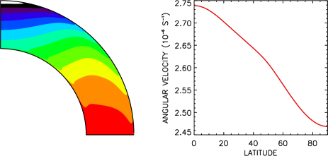
Figure 1: Differential rotation for nonmagnetic case is of the solar type. Angular velocity increases from poles to equator by about 10%.

Figure 2 shows how the global surface flow varies with the amplitude of prescribed poloidal field (13) for several latitudinal profiles of the field. As the field increases, the meridional flow reverses to poleward orientation and then grows steadily. When the flow becomes sufficiently fast, the differential rotation reverses to anti-solar case. We were able to follow the dependencies up to the value of order $B_{0}\sim 100...300$ G depending on the bottom profile (13) of the poloidal field. Our numerical code based on the relaxation method did not converge for stronger fields. The numerical instability, probably, signals on the onset of the physical flux-concentration instability (Kitchatinov & Mazur [2000]) via which the cool magnetic spots are formed. By this reason, we did not have true magnetic spots but smooth magnetically induced thermal inhomogeneities in our simulations.

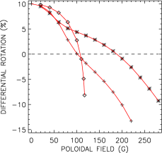
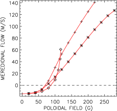
Figure 2: Left panel: surface differential rotation, $100\left(\Omega^{\rm eq}-\Omega^{\rm pole}\right)/\Omega_{0}$, as function of the poloidal field amplitude, $B_{0}$ (13). Actually computed points are marked by signs. Different signs correspond to different values of the $n$-parameter of the bottom profile (13) of the poloidal field: $n=1$ (diamonds), $n=3$ (crosses), $n=5$ (stars). Right panel: Surface meridional flow at 45^∘-latitude. Positive values mean poleward flow.

Figure 3 illustrates typical case of anti-solar rotation of present simulations. Angular velocity increases from equator to pole but not steadily. In agreement with above qualitative arguments, the increase occurs in the same latitude range where relatively fast poleward meridional flow can be observed in Fig. 4. The surface rotation of Fig. 3 cannot be approximated by traditional $\cos^{2}\vartheta$ profile. It may be reasonable to use higher-order terms in approximations of the observed anti-solar rotation laws. Expansion in terms of Gegenbauer polynomials (Rüdiger [1989]),

$$\Omega\left(\vartheta\right)=\sum_{n=1}^{N}{\omega_{n}\over\sin\vartheta}P_{2n-1}^{1}\left(\cos\vartheta\right),$$ (14)

may be convenient, especially when rotation law variations with time are concerned.

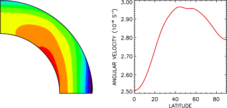
Figure 3: Simulated differential rotation for poloidal field amplitude $B_{0}=200$ G. Angular velocity increases from equator to pole by about 10%. Low and high latitudes have opposite sense of the latitudinal rotation inhomogeneity.

The meridional flow of Fig. 4 is driven by the barocline forcing due to the thermal depletion which occupies same region of latitudes. As was already mentioned, there were no true thermal spots in the simulations. Nevertheless, the thermal depletion of Fig. 4 was produced by magnetic quenching of convective heat flux of Eq. (8).

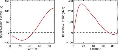
Figure 4: Left panel: Deviation of surface temperature from its mean value as a function of latitude for same model as Fig. 3. Right panel: surface meridional flow. $B_{0}=200$ G.

The magnetic field structure and amplitude are illustrated by Figs. 5 and 6. The poloidal field amplitude, $B_{0}=200$ G, is the mean value. Its maximum strength in the polar region is about 2.5 times larger. It is not poloidal field, however, which makes the principal influence on convective heat flux (8) and produces the temperature depletion of Fig. 4. The toroidal field of Fig. 6 is stronger by about one order of magnitude.

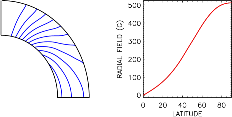
Figure 5: Left panel: lines of the poloidal magnetic field for same model as Fig. 3. Right panel: surface field strength.

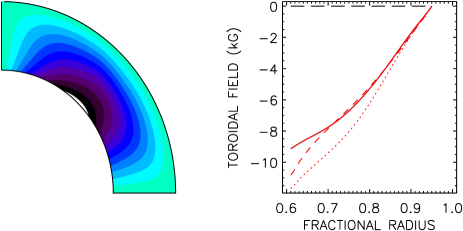
Figure 6: Toroidal magnetic field for same model as Fig. 3. Right panel shows radial profiles of the field for latitudes of 20^∘ (full line), 40^∘ (dotted), and 60^∘ (dashed).

The anti-solar rotation of Fig. 3 can be interpreted along the following sequence. Toroidal magnetic field of Fig. 6 produces thermal depletion of Fig. 4 by suppression of the convective heat flux (8). The thermal depletion drives a relatively fast meridional flow of Fig. 4 via the barocline forcing of Eq. (7). The meridional flow tends to make the angular momentum uniform along its stream-lines in accord with the solution (5) of the angular velocity equation (4) for the advection-dominated case thus producing relatively slow rotation of the equator. It should be noted, however, that convective fluxes of angular momentum (the $\Lambda$-effect, Rüdiger & Hollerbach [2004]) does also take part in formation of the differential rotation, and we return to the beginning of our interpretation by noticing that the toroidal magnetic field is produced from poloidal one by the differential rotation.

The simulated anti-solar rotation of preceding section is the first theoretical indication for this type of differential rotation. Nevertheless, it is tempting to notice points of yet qualitative agreement with observations of the giant star HD 31993 by Strassmeier et al. ([2003]). The star shows differential rotation of about 12% of anti-solar type. The dark spots were observed on low latitudes and they had temperature contrast of about 200^∘ K only which is compatible with (latitude-averaged) moderate temperature depletion of Fig. 4. In a further agreement, the observed star had a warm pole. It is not clear, however, whether meridional flow was as fast as required by our theoretical model to produce anti-solar rotation.

Unfortunately, HD 31993 remains the only giant star for which the anti-solar type of rotation was detected incontroversially. The other candidate, HD 199178, is under debates (Hackmann et al. [2001], Petit et al. 2004).

The anti-solar rotation was detected for six close binaries also (Strassmeier [2003]). Consideration of section 2 suggests this type of star as another possibility for equatorial deceleration though no quantitative model for binaries was developed so far.

5 What to observe?

It seems to be a quite general theoretical statement that relatively fast meridional flow should be present whenever differential rotation is of anti-solar type. Accordingly, it is fundamentally important to know whether observations can confirm that all stars showing relatively slow equatorial rotation do simultaneously possess a large meridional flow.

It is appropriate to estimate how fast the meridional circulation should be for producing the anti-solar differential rotation. Significance of meridional flow is defined by the Reynolds number, ${\rm Re}=u^{\rm m}R/\nu_{{}_{\rm T}}\simeq u^{\rm m}R\tau/\ell^{2}$ ($\ell$ and $\tau$ are mixing length and time respectively). Judging from Fig. 2, the poleward meridional flow of

$$u^{\rm m}\geq 30{\ell^{2}\over\tau R}$$ (15)

should be sufficient to support the equatorial deceleration. The fast circulation is expected to drive differential rotation of anti-solar type independently of whether the direction of the surface flow is towards pole or equator. Estimations by Rüdiger ([1989]) suggest, however, that equatorward flow should be several times faster compared to Eq. (15) to produce anti-solar rotation.

It may be noticed that the meridional circulation has been recognized as an important ingredient of stellar dynamos (Choudhuri et al. [1995], Dikpati & Gilman [2001], Bonnano et al. [2002]). Accordingly, observational detections of the meridional flow would be helpful for stellar dynamo theory also.

Another possibility for observational verification of the above theoretical predictions is to check whether all anti-solar rotators do indeed belong to one of two groups: spotted giants or close binaries. The suggestion that a fast meridional flow can be found only for the two groups of stars is, however, more speculative and less certain than the necessity of the meridional flow itself for rotation laws of anti-solar type.

Measuring differential rotation and meridional flow on giant stars can be a difficult observational task because of relatively long rotation periods of giants. The task may be a natural subject for robotic astronomy because long observational series may be required.