Oxygen isotopic ratios in galactic clouds along the line of sight towards Sagittarius~B2

As an independent check on previous measurements of the isotopic abundance of oxygen through the Galaxy, we present a detailed analysis of the ground state rotational lines of ¹⁶OH and ¹⁸OH in absorption towards the giant molecular cloud complex, Sagittarius B2. We have modelled the line shapes to separate the contribution of several galactic clouds along the line of sight and calculate ¹⁶OH/¹⁸OH ratios for each of these features. The best fitting values are in the range 320–540, consistent with the previous measurements in the Galactic Disk but slightly higher than the standard ratio in the Galactic Centre. They do not show clear evidence for a gradient in the isotopic ratio with galactocentric distance. The individual ¹⁶OH column densities relative to water give ratios of [H₂O/OH]=0.6–1.2, similar in magnitude to galactic clouds in the sight lines towards W51 and W49. A comparison with CH indicates [OH/CH] ratios higher than has been previously observed in diffuse clouds. We estimate OH abundances of 10^-7–10^-6 in the line of sight features.

1 Introduction

The OH radical is one of the key oxygen bearing species in the interstellar medium (ISM). Not only is it a good diagnostic of physical and chemical conditions (e.g. Goicoechea et al. 2005), but in addition, it provides a very good way to investigate the relative abundance of oxygen isotopes via its isotopologues ¹⁶OH, ¹⁸OH and ¹⁷OH. Chemical fractionation reactions that might distort the oxygen isotopic ratios in molecular species are not thought to be important (Langer et al. 1984) and this means that observations of OH can be used directly to determine the ratios ¹⁶O/¹⁸O and ¹⁸O/¹⁷O.

These values are important as they are set by stellar processing and outflow mechanisms and so constrain models of galactic chemical evolution (e.g. Prantzos et al. 1996). ¹⁶O is a primary product of stellar nucleosynthesis, produced directly from the primordial elements H and He (see Wilson & Matteucci 1992). Both ¹⁷O and ¹⁸O are secondary products which require heavier elements from previous nuclear burning for their production. Chemical evolution models (e.g. Prantzos et al. 1996) show that the primary/secondary ratios, ¹⁶O/¹⁷O and ¹⁶O/¹⁸O, should fall with decreasing galactocentric distance due to the increased processing rate towards the Galactic Centre. These ratios should also fall with time due to the build up of the secondary elements in the ISM.

Previous measurements of ¹⁶O/¹⁸O in the ISM have mainly been made via the radio lines of H₂CO and CO towards molecular clouds (see Wilson & Rood 1994). However, these lines are generally optically thick in the most abundant isotopologues and so double ratios such as H${}_{2}^{13}$C¹⁶O/H${}_{2}^{12}$C¹⁸O are used. This relies on accurate knowledge of ¹²C/¹³C which is subject to chemical fractionation in molecular species (e.g. Langer et al. 1984).

A very good way to get around these difficulties is to use the OH molecule - several measurements using its 18 cm $\Lambda$-doubling transitions have been made towards the Galactic Centre (Whiteoak & Gardner 1981; Williams & Gardner 1981), although in some circumstances these can be complicated by excitation effects within the hyperfine levels (Bujarrabal et al. 1983). This problem can be avoided by using the far-infrared (FIR) rotational lines which should not be affected by hyperfine excitation anomalies. These provide an excellent way to independently check the ratios determined at radio wavelengths.

Rotational transitions of OH have previously been studied towards the Orion Kleinmann-Low nebula using the Kuiper Airborne Observatory (Melnick et al. 1990, and references therein) where both ¹⁶OH and ¹⁸OH were used to constrain the physical conditions of the source. More recently, Goicoechea & Cernicharo (2002) have used the Infrared Space Observatory (ISO) satellite to observe OH in the envelope of the giant molecular cloud complex Sagittarius B2 (Sgr~B2). The lowest energy transitions show absorption due to both ¹⁶OH and ¹⁸OH in Sgr~B2 itself and in foreground features intersecting the line of sight. They indicate that the isotopic ratios are broadly similar to the previous radio results.

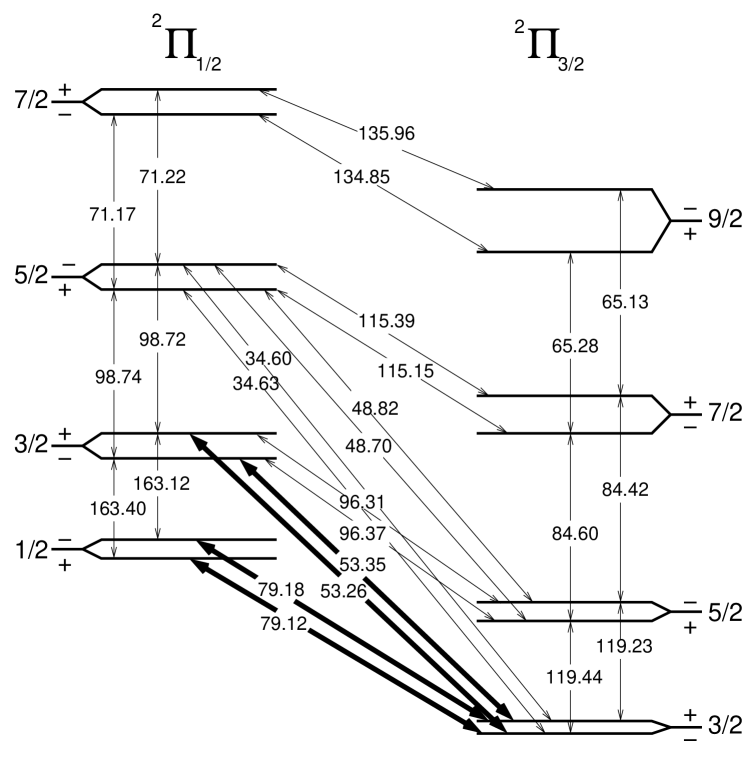
Figure 1: Low lying rotational energy levels in the electronic and vibrational ground state of the ¹⁶OH molecule, adapted from Brown et al. (1982). The $\Lambda$-doubling of each level is shown but the splitting has been exaggerated for clarity. The relative spacing of the levels in energy is only approximate. The $J$ values for each level are shown and the wavelength of each transition is given in $\mu$m. The transitions used in the analysis presented here are shown as thick arrows.

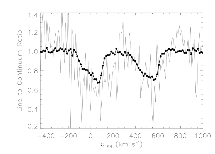
Figure 2: The ¹⁶OH ${}^{2}\Pi_{1/2}$–${}^{2}\Pi_{3/2}$ $J$=3/2–3/2 transition at 53.26 $\mu$m from non-prime data (black) and prime data (grey). Both datasets are binned at 1/4 of their respective resolution elements (non-prime: 61 km s^-1 and prime: 45 km s^-1). The gain in signal-to-noise in the non-prime data is a factor of $\sim$9.

In this paper we conduct a more detailed investigation into ISO observations towards Sgr~B2, with the aim of separating the relative abundances of ¹⁶OH and ¹⁸OH in individual absorption components in the line of sight. A similar comparison of ¹⁸OH with ¹⁷OH has already been presented by Polehampton et al. (2003). We have used data from a wide spectral survey carried out with the ISO Long Wavelength Spectrometer (LWS; Clegg et al. 1996) Fabry-Pérot mode. A combination of prime and non-prime data from the survey allowed us to increase the signal-to-noise ratio over the standard data and derive an accurate and consistent calibration for two ground state transitions of ¹⁶OH and one transition of ¹⁸OH.

After presenting the observations and results, we describe a model of the line shape to separate the line of sight absorption into 10 velocity components (Sect. 4). In Sect. 5 we assign the ¹⁶OH/¹⁸OH ratio for each component to a galactocentric distance and compare with previous determinations of the isotopic abundances. We discuss the final ¹⁶OH column densities in relation to other related species in Sect. 6.

2 Observations and data reduction

Sgr~B2 was observed as part of a wide spectral survey using the ISO LWS Fabry-Pérot (FP) mode L03. Unbiased coverage of the whole LWS spectral range (47–196 $\mu$m) was carried out using 36 separate observations with a spectral resolution of $30$–$40$ km s^-1. No other object outside of the Solar System was observed over the complete LWS spectral range in this way. Results from this survey have been presented by Ceccarelli et al. (2002); Polehampton et al. (2002a); Vastel et al. (2002); Polehampton et al. (2003, 2005). Sgr~B2 was also extensively observed by the LWS FP in narrow wavelength scans using the L04 mode (see Goicoechea et al. 2004). We have used several of these L04 observations to improve the signal-to-noise ratio in the L03 data for ¹⁸OH. The ISO TDT numbers for all the observations used in this paper are detailed in Table 3.

The LWS beam had an effective diameter of approximately 80$\arcsec$ (Gry et al. 2003) and L03 observations were pointed at coordinates $\alpha=17^{\mathrm{h}}47^{\mathrm{m}}21.75^{\mathrm{s}}$, $\delta=-28\degr 23\arcmin 14.1\arcsec$ (J2000). This gave the beam centre an offset of 21.5$\arcsec$ from the main FIR peak at Sgr~B2~(M) - this pointing was used to exclude the source Sgr~B2~(N) from the beam. The additional L04 observations were pointed directly towards the nominal position of Sgr~B2~(M), but careful comparison showed no significant difference to the L03 observations. Each observation had a spectral sampling interval of 1/4 resolution element with each point repeated 3–4 times in L03 mode and 11–15 times in L04 mode.

Figure 3: Data for the ¹⁶OH cross ladder (${}^{2}\Pi_{1/2}$–${}^{2}\Pi_{3/2}$) transitions, $J$=1/2–3/2 at 79 $\mu$m (left; binned at 1/4 resolution element) and $J$=3/2–3/2 at 53 $\mu$m (right; binned at $\sim$1/6 resolution element), plotted as line to continuum ratio. The errors shown represent the combined statistical and systematic uncertainty in each bin. The two $\Lambda$-doublet components have been averaged for the 53 $\mu$m line. The best fitting model accounting for the absorbing clouds in the line of sight is shown as the solid line (see text).

In addition to the primary spectral survey data, each line was generally included in at least one other L03 observation. This occurred because the LWS used 10 detectors, which always recorded data in their own spectral ranges (the prime observations consist of data from a single detector for which instrument settings were optimised). We have included these ’non-prime’ data to further improve the signal-to-noise ratio.

Each observation was carefully reduced using the LWS offline pipeline (OLP) version 8 (for FP data the difference between OLP version 8 and the latest version 10 is not significant). Further processing was then carried out interactively using routines that appeared in the LWS Interactive Analysis package version 10 (LIA10: Lim et al. 2002) and the ISO Spectral Analysis Package (ISAP: Sturm et al. 1998). The method included determination of accurate dark currents (including stray light), interactive division of each mini-scan by the LWS grating response profiles and careful scan by scan removal of glitches (see Polehampton et al. 2002a, 2003).

Before co-adding the data for each line, the wavelength scale of each observation was corrected to the local standard of rest (LSR). Non-prime observations were carefully checked against the equivalent prime measurement to align the line centres. This is particularly important for non-prime data measured with the LWS long wavelength FP (FPL) below 70 $\mu$m (outside its nominal operating range) because the standard FPL wavelength calibration did not include short wavelength data (Gry et al. 2003). For the ¹⁶OH $J$=3/2–3/2 cross ladder transition at 53 $\mu$m (Fig. 1 shows the energy levels for OH), we have used only non-prime FPL data. This is because it has a significantly higher signal-to-noise ratio than the prime data (due to the higher transmission of FPL compared to the short wavelength FP, FPS; Polehampton et al. 2002b). The absolute wavelength alignment was difficult to determine purely by comparison with the noisy prime data and so a velocity shift was allowed as a free parameter in the modelling (see Sect. 4.1). Figure 2 shows the resulting shift cross-checked with the prime data. The gain in signal-to-noise achieved by using FPL rather than FPS is approximately a factor of 9. The only cost in using these data is a reduction in spectral resolution from 45 km s^-1 (for FPS) to 61 km s^-1 (for FPL).

After co-addition, the continuum around each line was fitted with a 3rd order polynomial baseline which was then divided into the data to obtain the relative depth of the lines below the continuum. This effectively bypassed the large systematic uncertainties in the multiplicative calibration factors needed to obtain the absolute flux scale (see Swinyard et al. 1998). The remaining errors are due to detector noise, uncertainty in the dark current and the polynomial fit.

At the resolution of the LWS, two components are visible for each OH transition due to the $\Lambda$-doublet type splitting of each rotational level. However, further hyperfine splitting is not resolved. The two $\Lambda$-doublet components showed good agreement in the data, and so where they were well separated (the $J$=3/2–3/2 cross ladder transition at 53 $\mu$m for ¹⁶OH and the $J$=5/2–3/2 transition at 120 $\mu$m for ¹⁸OH), they were co-added to further increase the signal-to-noise ratio.

3 Results

Figure 1 shows the low-lying rotational transitions of ¹⁶OH, most of which are included in the spectral survey range. The strongest lines observed in the survey were due to the ${}^{2}\Pi_{3/2}\leavevmode\nobreak\ J$=5/2–3/2 transition from the ground state at 119 $\mu$m. These lines show almost complete absorption of the FIR continuum in the range $-150$ to $+100$ km s^-1 (see Goicoechea & Cernicharo 2002). Due to the large depth of the lines, the shape was strongly affected by the transient response of the LWS detectors. These detector memory effects (see Lloyd 2002) meant that successive repeated scans underestimated the depth and the continuum level following each line. Therefore, the lines were not used in the analysis presented here. There are two remaining transitions from the ground rotational state (see Fig. 1) that occur between the ${}^{2}\Pi_{3/2}$ and ${}^{2}\Pi_{1/2}$ ladders: $J$=1/2–3/2 at 79 $\mu$m and $J$=3/2–3/2 at 53 $\mu$m. These lines are also broad but with much lower optical depth. They are shown in Fig. 3. The broad absorption is due to features between the Sun and Galactic Centre associated with galactic spiral arms that cross the line of sight (e.g. Greaves & Williams 1994).

Several ¹⁶OH transitions between higher energy rotational levels are observed in the survey at the velocity of Sgr~B2 itself but do not occur in the line of sight clouds. These lines originate in the envelope of Sgr~B2 and have been modelled by Goicoechea & Cernicharo (2002). They show that the excited OH originates in clumpy photodissociation regions (PDRs) on the edge of the Sgr~B2 complex at temperatures of 40–600 K. In this paper, we concentrate on the broad absorption observed in the ground state lines at 79 and 53 $\mu$m.

Due to the lower abundance of ¹⁸OH, the fundamental ground state ${}^{2}\Pi_{3/2}\leavevmode\nobreak\ J$=5/2–3/2 transition is much weaker and the cross-ladder and higher energy lines are not detected. Figure 4 shows the $J$=5/2–3/2 line after co-adding the two resolved $\Lambda$-doublet components. These observations were previously presented by Polehampton et al. (2003). Here we have used additional data from the L04 mode, which showed good agreement with the L03 data.

Figure 4: Co-added data from the two $\Lambda$-doublet components of the ¹⁸OH ${}^{2}\Pi_{3/2}\leavevmode\nobreak\ J=5/2$–$3/2$ transition. The data were binned at 1/4 resolution element and the errors represent the combined statistical and systematic uncertainty in each bin. The best fitting model accounting for absorbing clouds in the line of sight is shown (see text).

4 Modelling of OH in the line of sight

4.1 High resolution model

At the spectral resolution of the LWS, the line of sight components are blended together into a single broad absorption. We have modelled the line shape using higher spectral resolution measurements to fix the velocities and widths of each component. Comparison of high resolution spectra tracing molecular and atomic species in these clouds show very similar line widths and velocities (CO; e.g. Vastel et al. (2002), H₂CO; e.g. Mehringer et al. (1995), HI; e.g. Garwood & Dickey (1989)). These tracers also show a very similar velocity structure to observations of the $\Lambda$-doubling lines of OH at cm wavelengths (McGee et al. 1970; Whiteoak & Gardner 1975, 1981; Williams & Gardner 1981; Bujarrabal et al. 1983).

We have assumed that the H i measurements are a representative tracer and based our model on the published parameters from Garwood & Dickey (1989) (after correcting an error in their Table 2: 11 km s^-1 should read 1.1 km s^-1). This method has already been used to successfully fit the absorption of CH and CH₂ (Polehampton et al. 2005) and is similar to the method used to fit O i and C ii lines by Vastel et al. (2002).

The H i observations were made using the VLA pointed close to Sgr~B2~(M). In our model, the H i data were used to fix the velocity and line width of 10 line of sight features with each component assumed to have a Gaussian line shape. The optical depth at each velocity, $\tau$, was then adjusted as a free parameter and the line-to-continuum ratio calculated from,

$$I=I_{c}\exp{(-\tau)}$$ (1)

where $I_{c}$ is the intensity of the continuum. The resulting spectrum was then convolved to the resolution of the LWS. In order to put the best constraint on the line shape, the two ¹⁶OH lines were fitted simultaneously with the ¹⁸OH line. Optical depths were varied in the model for the 79 $\mu$m line and then used to calculate the shape of 53 $\mu$m line assuming that both lines trace the same column density. This must be true as they originate in the same lower level. Column densities were calculated assuming a Doppler line profile with Maxwellian velocity distribution (e.g. Spitzer 1978),

$$N_{j}=\frac{8\pi\sqrt{\pi}}{2\sqrt{\ln 2}}\leavevmode\nobreak\ 10^{17}\leavevmode\nobreak\ \frac{\tau_{0}\leavevmode\nobreak\ \Delta{v}}{A_{i\,j}\leavevmode\nobreak\ \lambda_{i\,j}^{3}\leavevmode\nobreak\ g_{i}/g_{j}}$$ (2)

where $N_{j}$ is the column density in the lower level in cm^-2, $\tau_{0}$ is the optical depth at line centre, $\Delta{v}$ is the line width in km s^-1, $A_{ij}$ is the Einstein coefficient for spontaneous emission in s^-1, $\lambda_{ij}$ is the wavelength in $\mu$m and $g_{i}$ is the statistical weight of state $i$. The line wavelengths and Einstein coefficients used (averaged over the unresolved hyperfine structure) are shown in Table 4.

Further free parameters were added to the fit describing the ¹⁶OH/¹⁸OH column density ratio, allowing the shape of the 120 $\mu$m ¹⁸OH line to be calculated. Clouds which are thought to reside at similar galactocentric distances were forced to have identical isotope ratios - this affects the features at $-108/-82$ km s^-1, $-52/-44$ km s^-1 and $+53/+67$ km s^-1. In order to account for any drift in the wavelength calibration between the lines, a free velocity shift was allowed for each line, giving a total of 20 free parameters in the fit. The most important factor constraining the velocity shift was the relatively deep and narrow absorption at the velocity of Sgr~B2 in the ¹⁸OH line. The Numerical Recipes multi-parameter fitting routine, ‘amoeba’ (Press et al. 1992), was used to minimise $\chi^{2}$.

Table 1: Column densities and ¹⁶OH/¹⁸OH ratios for the best fit carried out to the ¹⁶OH and ¹⁸OH ground state lines. Columns 1 and 2 show the Gaussian fit parameters from the H i observations of Garwood & Dickey (1989).

Velocity	FWHM	$N(\mathrm{{}^{16}OH})$	16OH/18OH
(km s-1)	(km s-1)	($10^{15}$ cm-2)
$-108\pm 2$	$7\pm 4$	$0.56\pm 0.39$	$460^{+90}_{-50}$
$-82\pm 4$	$28\pm 12$	$9.0\pm 3.9$	$460^{+90}_{-50}$
$-44.0\pm 0.6/(-52\pm 6)^{a}$	$8\pm 2$ ($17\pm 5$)	$3.5\pm 1.8$	$450^{+100}_{-60}$
$-24.4\pm 0.8$	$14\pm 2$	$5.4\pm 1.8$	$370^{+110}_{-50}$
$+1.1\pm 0.4$	$19\pm 1$	$7.6\pm 3.4$	$430^{+80}_{-40}$
$+15.7\pm 0.3$	$7\pm 1$	$3.6\pm 2.3$	$360^{+80}_{-50}$
$+31\pm 4$	$21\pm 14$	$5.4\pm 3.8$	$540^{+100}_{-50}$
$+66.7\pm 0.5/(+52.8\pm 0.9)^{b}$	$16\pm 1$ ($11\pm 2$)	$32^{+6}_{-4}$	$320^{+70}_{-30}$
Total		67.0

^a These two components are too close to separate in our model and the best fit line shape requires only the $-44.0$ km s^-1 component.
^b The H i data resolve 2 components in Sgr~B2. However, our fit requires only one of these (at 66.7 km s^-1) to reproduce the ISO spectrum.

In order to ensure that the algorithm did not converge at a false minimum, the initial conditions were set close to their best values and the routine was restarted at the first convergence point. Solutions with negative absorption were avoided by setting $\chi^{2}$ to be high when the optical depth went below zero.

The best fitting model is shown plotted with the data for each line in Figs. 3 and 4. The final ¹⁶OH column densities and ¹⁶OH/¹⁸OH ratios are shown in Table 1. In the line of sight clouds where no absorption is observed from higher energy levels (Goicoechea & Cernicharo 2002), the ground state population is a good measure of the total OH column density. The fitted components are all optically thin except at the velocity of Sgr~B2 itself, where optical depths of 2.5–3.3 were found for the ¹⁶OH lines. However, these are not high enough to break the assumption of purely Doppler line profiles used in the model and calculation of column densities.

The best fitting velocity shift applied to the ¹⁶OH $J$=1/2–3/2 line at 79 $\mu$m was 8.8 km s^-1 and for the ¹⁸OH $J$=5/2–3/2 line at 120 $\mu$m was $-1.9$ km s^-1. These shifts centred the deepest absorption on the H i component at $+67$ km s^-1 and are within the uncertainty in FP wavelength calibration ($<11$ km s^-1; Gry et al. 2003). However, for the ¹⁶OH $J$=3/2–3/2 line at 53 $\mu$m using data taken with non-prime detectors, a larger shift of 28 km s^-1 was required. This shift is due to the fact that this line was observed with FPL outside of its nominal range (see Sect. 2). In order to determine if this large velocity offset was reasonable, we compared the shifted data to the noisier prime observation (in which the accuracy of the wavelength calibration should be better than 6 km s^-1; Gry et al. 2003). The two line components show good agreement (see Fig. 2) and the line shift is consistent with that found for other spectral lines observed using FPL below 70 $\mu$m (Polehampton 2002).

The final fit shows that only 8 of the 10 velocity components are necessary to reproduce the observed line shape. At the velocity associated with Sgr~B2, the width of the absorption in the ¹⁸OH line is too narrow to allow strong absorption by both the $+53$ and $+67$ km s^-1 components observed for H i. This is consistent with the results obtained by fitting the ground state line of CH (Polehampton et al. 2005). Also, the two components at $-52$ and $-44$ km s^-1 are too closely spaced to be separated in our fit and significant optical depth was found only at $-44$ km s^-1 (in Table 1, only one value centred at $-44$ km s^-1 is given for the two components).

We have also investigated the effect of further reducing the number of fit components in order to increase confidence in the final column densities and ratios. The minimum number of components that can reasonably be fitted to the spectrum is 4 (e.g. following Neufeld et al. 2000). We re-ran our model using 4 velocity components corresponding to the ranges used by Neufeld et al. and widths estimated from their H${}_{2}^{18}$O spectrum observed with the Submillimeter Wave Astronomy Satellite (SWAS). These 4 empirically determined components can broadly reproduce the observed line shapes. The fit gives ¹⁶OH column densities and ¹⁶OH/¹⁸OH ratios that are within the errors of the results from Table 1 summed in the relevant velocity ranges. The ¹⁶OH/¹⁸OH ratios obtained are, 480 (centred at $-80$ km s^-1), 470 (centred at $-40$ km s^-1), 510 (centred at $+10$ km s^-1) and 290 (centred at $+65$ km s^-1). However, we have used the high resolution H i observations as a basis for our model because this can not only fully describe the line shapes but also allows the contribution of clouds at different galactocentric distances along the line of sight to be disentangled.

4.2 Errors on fitted parameters

The number of closely spaced velocity components in the fit made the modelling difficult as their separation was less than the resolution of the LWS. This meant that variation in one component could be compensated for by changing another, resulting in a relatively large uncertainty in each fitted optical depth. In addition, the results for each component are likely to be an average over several closely spaced narrow features such as those observed showing CS absorption with velocity widths $\sim$1 km s^-1 (Greaves & Williams 1994). However, this would only alter the total column densities if a few of the narrow features had very much higher optical depths than the others, and this does not appear to be the case in the CS data.

In order to estimate the uncertainty on each fitted parameter we performed a Monte-Carlo error analysis. The best fitting model determined by minimising $\chi^{2}$ was used to generate a set of synthetic spectra where each point had a mean value equal to the best fit and standard deviation equal to the original data error. We re-fitted each synthetic spectrum using the original fitting method and analysed the resulting dataset for each parameter. The results show that the errors on neighbouring optical depths are strongly correlated, but that these are not correlated with the uncertainty in ¹⁶OH/¹⁸OH ratios (except for the Sgr~B2 component). This is due to the fact that the best fit isotopologue ratios depend more on the overall line shape than on the relative optical depth in neighbouring components. The final uncertainty in column density is shown in Table 1 as a combination of 1$\sigma$ errors in H i line width (as quoted by Garwood & Dickey 1989) and the modelling errors in optical depth. The errors in ¹⁶OH/¹⁸OH ratio were determined directly from the Monte-Carlo analysis.

4.3 Comparison with previous results

The column density at the velocity of Sgr~B2 has previously been calculated by Goicoechea & Cernicharo (2002) using ISO FP data observed in the L04 mode. They used a radiative transfer model and accounted for the populations in higher energy levels up to 420 K above ground to determine $N(^{16}\mathrm{OH})=(1.5$–$2.5)\times 10^{16}$ cm^-2. Lower resolution observations with the LWS grating mode show that OH is widespread across the whole Sgr~B2 region with column densities in the range (2–5)$\times 10^{16}$ cm^-2 (Goicoechea et al. 2004). Our value associated with Sgr~B2 from Table 1 gives $N(^{16}\mathrm{OH})=(3.2^{+0.6}_{-0.4})\times 10^{16}$ cm^-2 in the ground state level. This is slightly higher than the previous FP result but fits into the general picture reasonably well. We also find a slightly higher value than Goicoechea & Cernicharo (2002) for $N(^{18}\mathrm{OH})$: $(9.8\pm 1.6)\times 10^{13}$ cm^-2 compared to $(6\pm 2)\times 10^{13}$ cm^-2.

The column density of ¹⁶OH has also been measured from observations of its $\Lambda$-doubling lines at 18 cm. Bieging (1976) used the interferometer of the Owens Valley Radio Observatory (OVRO) to calculate an integrated column density over the velocity range 40–89 km s^-1 equal to $1.2\times 10^{17}$ cm^-2. This would indicate that the FIR lines underestimate the column density by a factor of 4. However, if the excitation temperature of the 18 cm lines is less than the assumed 20 K (see the discussion in Stacey et al. 1987), the radio column density could be an over-estimate. Also, the 18 cm lines may sample a different component of the envelope as the depth at which the continuum is emitted occurs deeper into the cloud than in the FIR region, and the OVRO synthesised beam ($3.25\arcmin$) is larger than that of ISO. Bieging (1976) estimates that the column density in the negative velocity features is smaller than the positive velocity values by about a factor of four.

The total column density of ¹⁸OH over the whole line of sight in our fit was $(1.8\pm 0.2)\times 10^{14}$ cm^-2 and this compares favourably with previous observations using the Kuiper Airborne Observatory: Lugten et al. (1986) found a total column density of $N(^{18}\mathrm{OH})\geq 2\times 10^{14}$ cm^-2.

Figure 5: Values of ¹⁶OH/¹⁸OH from Table 1 plotted against distance from Galactic Centre (large circles with cross). The velocity of each component is indicated in km s^-1 next to each point. The compilation of values from Kahane (1994) is plotted for comparison, as well as the best fitting galactic gradient found by Wilson & Rood (1994).

5 ¹⁶OH/¹⁸OH ratio

Table 1 gives the best fitting ¹⁶OH/¹⁸OH ratios. In order to compare with previous measurements of the isotopic ratios, a galactocentric distance must be assigned to each feature. Several of the velocity components have been well established to come from galactic spiral arm and Galactic Centre features such as the Galactic Bar at large negative velocities (Scoville 1972), the 3 kpc expanding arm at $-44$ km s^-1 (e.g. Burke 1965), the 4-5 kpc arm at $-24$ km s^-1 (Menon & Ciotti 1970) and Sgr~B2~(M) itself at $+50$–70 km s^-1 (e.g. Martín-Pintado et al. 1990). Associations for the remaining features have been proposed by Greaves & Williams (1994). In this case, the 1, 16 and 31 km s^-1 features would be associated with local spiral arms. However, it has been suggested that there may be a contribution at 0 km s^-1 by gas associated with Sgr~B2 (e.g Gardner et al. 1988).

Figure 5 shows our results plotted against their distances from the Galactic Centre taken from Greaves & Williams (1994). Compilations of many observations of H₂CO through the Galaxy indicate that there is a gradient in the ¹⁶O/¹⁸O ratio with decreasing values towards the Galactic Centre (Tosi 1982; Wilson & Rood 1994; Kahane 1994). The best fit gradient found by Wilson & Rood (1994) is overplotted in Fig. 5 as well as the compilation of H₂CO and CO results from Kahane (1994).

The three most uncertain distances are for the local components. At 31 km s^-1 we find a relatively high value of ¹⁶OH/¹⁸OH, consistent with its location close to the Sun. At 1 km s^-1, our value is in good agreement with that found from OH $\Lambda$-doublet lines of 440 (Bujarrabal et al. 1983). However, both the 1 and 16 km s^-1 components have rather lower values than might be expected for local gas. The gradient of Wilson & Rood (1994) predicts a local value of $560\pm 25$, although it has been measured to be even higher using HCO⁺ absorption by Lucas & Liszt (1998), giving $672\pm 110$. This may indicate that the local absorbing gas towards Sgr~B2 has atypical isotopic abundances. An anomalously low ¹²C/¹³C ratio has also been found in this gas by Greaves (1995). She rules out an error in the distance estimate and attributes the extra ¹³C to enrichment by stellar ejecta containing secondary nucleosynthesis products. In this case it would be natural to also find a higher abundance of ¹⁸OH.

In comparison, the standard Solar System abundance (derived from Standard Mean Ocean Water) is (¹⁶O/¹⁸O)${}_{\mathrm{SMOW}}=498.7\pm 0.1$ (Baertschi 1976). The value in the outer layers of the Sun has been measured to be ¹⁶O/${}^{18}\mathrm{O}=440\pm 50$ (Harris et al. 1987) and in the Solar wind, Collier et al. (1998) found ¹⁶O/${}^{18}\mathrm{O}=450\pm 130$. This should represent the conditions when the Sun was formed and models predict that it should be higher than the current ratio in the local ISM due to the build up of secondary elements from stellar processing (e.g. Prantzos et al. 1996). In order to explain the low Solar System abundances compared to the ISM, it has been proposed that the Sun was formed closer to the Galactic Centre (Wielen & Wilson 1997).

In the Galactic Centre, the isotope ratio is generally taken to be 250 (Wilson & Rood 1994). This low value has been derived from measurements of the $\Lambda$-doublet lines of ¹⁶OH and ¹⁸OH (e.g. Williams & Gardner 1981; Whiteoak & Gardner 1981). However, Bujarrabal et al. (1983) show that the ¹⁶OH/¹⁸OH opacity ratio derived from the radio lines is only a good measure of the actual abundance ratio in cold clouds with kinetic temperatures $\leq$20 K. This is due to excitation anomalies in the hyperfine levels caused by rotational pumping by the FIR lines. This certainly occurs at the velocity of Sgr~B2 as can be seen from the higher energy lines of ¹⁶OH which show absorption within the ${}^{2}\Pi_{3/2}$ ladder but emission within the ${}^{2}\Pi_{1/2}$ ladder (Goicoechea & Cernicharo 2002). This would cause the previously derived isotopic ratios to underestimate the true value. At the velocity of Sgr~B2, our fit gives a ratio of 320${}^{+70}_{-30}$. This appears to confirm the suggestion of Bujarrabal et al. (1983) that the ratio in the Galactic Centre has been underestimated (assuming the same excitation conditions exist for ¹⁶OH and ¹⁸OH and the ground state ratio accurately reflects the isotopic abundance). We also find a high value for the component attributed to the Galactic Bar ($-108$ km s^-1) of 460${}^{+90}_{-50}$. Bujarrabal et al. (1983) find a ratio of $\simeq$370 in this component.

In contrast, measurements of other molecules in Sgr~B2 seem to agree with the lower radio OH values. However, none of these methods are easy to directly interpret and so may also underestimate the true value. Both H₂CO and CO must be used in a double ratio, relying on an accurate value of ¹²C/¹³C. Henkel et al. (1983) calculate ¹⁶O/¹⁸O$\sim$200 from measurements of H${}_{2}^{13}$C¹⁶O/H${}_{2}^{12}$C¹⁸O, although the final value is uncertain due to the correction for radiation trapping in H${}_{2}^{12}$C¹⁶O (used to determine the associated ¹²C/¹³C ratio). Observations of CO indicate a value of 250$\pm$100 in the Galactic Centre (Penzias 1981) but this may be affected by chemical fractionation of ¹³C (Penzias 1983). Gardner et al. (1989) have observed CH${}_{3}^{16}$OH and CH${}_{3}^{18}$OH towards Sgr~B2 leading to an isotopic ratio of 210$\pm$40. This does not include a correction for radiation trapping which would increase the ratio. Nummelin et al. (2000) calculate even lower ratios from S¹⁶O/S¹⁸O (120${}^{+58}_{-54}$) and S¹⁶O₂/S¹⁶O¹⁸O (112${}^{+26}_{-22}$). They explain these by assuming that the observed emission originates in the central regions of the Sgr~B2 complex where ¹⁸O could be enhanced by the ejecta from massive stars. Our FIR absorption measurements trace gas in the outer parts of the Sgr~B2 envelope.

Without low values at the Galactic Centre, our results show a much less convincing gradient than that obtained from the CO and H₂CO measurements. However, we have low number statistics and the distances of some components from the Galactic Centre are not very well known. There also must be some effect from a real variation in clouds at the same galactocentric distance, as indicated by the anomalous ¹⁶OH/¹⁸OH and ¹²C/¹³C at 0 km s^-1. This means that a larger sample is necessary to accurately confirm the trend through the Galaxy.

6 Comparison with other species

Table 2: Ratio of our derived ¹⁶OH column densities with those of CH from Polehampton et al. (2005) for each of the velocity components from Table 1.

Velocity	[16OH/CH]
(km s-1)
$-108$	$6.2\pm 6.5$
$-82$	$35\pm 21$
$-52$/$-44.0$	$19\pm 15$
$-24.4$	$28\pm 11$
$+1.1$	$38\pm 18$
$+15.7$	$12\pm 8$
$+31$	$36\pm 35$
$+52.8$/$+66.7$	$34\pm 7$

Several other related species have been observed in the line of sight clouds towards Sgr~B2. Observations of absorption due to the H${}_{2}^{16}$O and H${}_{2}^{18}$O ground state rotational lines have been made using SWAS (Neufeld et al. 2000). Although H${}_{2}^{16}$O completely absorbs the continuum, they calculate column densities in three line of sight velocity ranges from H${}_{2}^{18}$O. Both OH and H₂O are formed by the dissociative recombination of H₃O⁺ (H₃O⁺ is also observed to show absorption in the line of sight clouds; Goicoechea & Cernicharo 2001). Neufeld et al. (2002) show that if recombination of H₃O⁺ is the only production mechanism, the ratio of OH to H₂O gives good constraints on the branching ratios. However, they also show that in warm gas, neutral-neutral reactions can alter the balance. A further effect is the inclusion of grain surface reactions, which can increase the gas-phase abundance of H₂O whilst OH is relatively unaffected (Plume et al. 2004).

Using the ortho-H${}_{2}^{18}$O column densities from Neufeld et al. (2000) with an ortho-to-para ratio of 3 and our ¹⁶O/¹⁸O ratios averaged in their velocity ranges gives [H₂O/OH] ratios of 0.6–1.2 towards Sgr~B2. These values are a similar order of magnitude to those previously derived for line of sight absorption features towards W51 ($\sim$0.3; Neufeld et al. 2002) and W49 (0.26, 0.43; Plume et al. 2004), indicating a high branching ratio for H₂O and/or the necessity of including other processes such as gas-grain interactions. In gas at the velocity of Sgr~B2 itself, Goicoechea & Cernicharo (2002) have derived even higher values of [H₂O/OH]$\sim$1-10. In this case, there is probably a warm gas component present and neutral-neutral reactions could be important.

In diffuse clouds, CH has been observed to be tightly correlated with OH, with a column density ratio, [OH/CH]$\sim$3 (e.g. Liszt & Lucas 2002). Absorption from the ground state rotational transition of CH was observed as part of the ISO spectral survey towards Sgr~B2 and has been fitted in a similar way to the OH lines (Polehampton et al. 2005). Table 2 shows the ratio of our fitted ¹⁶OH column densities those of CH in each velocity component. These have a large uncertainty but seem to indicate values that could be up to ten times higher than that seen in diffuse clouds. This increased ratio cannot be caused by CH because the abundances found are very similar to diffuse cloud models (Polehampton et al. 2005). We can estimate the abundance of OH in the line of sight clouds using molecular hydrogen column densities in the range 4 to 14$\times 10^{21}$ cm^-2 (see Greaves & Nyman 1996). This leads to OH abundances 10^-7–10^-6 in these features. At the velocity of Sgr~B2, Goicoechea & Cernicharo (2002) find an abundance of (2–5)$\times 10^{-6}$. These abundances are much higher than found in diffuse clouds (models of diffuse clouds predict $X$(OH)$\sim 10^{-8}$; van Dishoeck & Black 1986) and lead to the high [OH/CH] ratio. Such high abundances of OH can be found in PDR regions.

7 Summary

In this paper we have presented an analysis of ¹⁶OH and ¹⁸OH FIR rotational lines towards Sgr~B2. Absorption at different velocities along the line of sight allowed us to calculate the ¹⁶OH/¹⁸OH ratio between the Sun and Galactic Centre.

The advantages of this technique for determining the isotopic ratio of oxygen are:

• Chemical fractionation effects are not important for ¹⁶OH and ¹⁸OH. Therefore the molecular column density ratio directly measures the isotope abundance.

• There are optically thin lines present from both species.

• The final ratio does not depend on the value of ¹²C/¹³C as for previous H₂CO and CO measurements.

• Uncertainties in the population of hyperfine states do not affect the final ratios (as they do for radio observations of $\Lambda$-doublet transitions).

• Only ground state lines are seen for the line of sight clouds, showing that excitation effects are not important in these clouds.

• All observations come from a single dataset with consistent and stable calibration over lines of both isotopologues.

The main disadvantage is the relatively low spectral resolution compared to the velocity separation of line of sight components. This introduced errors for individual components in the line shape modelling. However, the data used here allowed us to maximise confidence in the observed line shapes by combining several observations and with the good coverage of baselines around the lines.

We find ¹⁶OH/¹⁸OH ratios broadly consistent with previous isotopic abundances, although our results do not provide such clear evidence for a gradient of the ratio through the Galaxy (but they do not rule it out). In velocity components associated with the Galactic Centre, we find slightly higher ratios than previous results. This could be due to an underestimate in the previous radio observations of OH caused by pumping of hyperfine levels by the FIR rotational transitions (see Bujarrabal et al. 1983).

In comparing the total ¹⁶OH column densities with those of H₂O towards Sgr~B2, we find similar magnitude abundance ratios as have been seen in other lines of sight towards W51 and W49 (Neufeld et al. 2002; Plume et al. 2004). A comparison of ¹⁶OH with the column density of CH shows a wide scatter and large error, but appears to indicate higher ratios that previously observed in diffuse clouds.

This study shows that FIR rotational lines are an extremely useful tool for examining the variation of isotopic ratios in the ISM. The column densities of OH can be accurately derived as the method avoids the anomalous excitation that may be present in radio $\Lambda$-doublet lines. Ideally, future observations at higher spectral resolution are required to improve on the results. This may be possible using future telescopes such as SOFIA.

Appendix A Observations and wavelengths

Table 3: Log of the observations used.

Transition	Observing	ISO	LWS	Spectral	Repeated
	Mode	TDT	Detector	Resolution	scans
		Number		(km s-1)
16OH
${}^{2}\Pi_{3/2}\leavevmode\nobreak\ J$=5/2–3/2 (119 $\mu$m)	L03	50601013	LW2	33	3
${}^{2}\Pi_{1/2}$–${}^{2}\Pi_{3/2}$	L03	50400823	SW2	61	3
$J$=3/2–3/2 (53 $\mu$m)	L03	50601013	SW2	61	3
	L03	50700707	SW2	61	3
	L03	50800317	SW2	61	3
${}^{2}\Pi_{1/2}$–${}^{2}\Pi_{3/2}$	L03	50900521	SW5	40	3
$J$=1/2–3/2 (79 $\mu$m)	L03	50600814	SW5	40	3
	L03	50600603	SW4	40	3
	L03	50700208	SW4	40	3
	L03	83800606	SW4	40	4
	L03	50600506	SW4	40	3
18OH
${}^{2}\Pi_{3/2}\leavevmode\nobreak\ J$=5/2–3/2 (120 $\mu$m)	L03	50601013	LW2	33	3
	L03	50700610	LW2	33	3
	L04	49401705	LW2	33	15
	L04	46201118	LW2	33	11
	L04	46900332	LW2	33	14

Table 4: Wavelengths and Einstein coefficients ($A_{ij}$) for ¹⁶OH and ¹⁸OH averaged over hyperfine structure. The ¹⁶OH wavelengths are from Brown et al. (1982) and Varberg & Evenson (1993) and the Einstein coefficients were calculated from the line strengths of Brown et al. (1982). The ¹⁸OH wavelengths are from Morino et al. (1995) with Einstein coefficients calculated from the line strengths of Comben et al. (1986).

Transition	Wavelength	$A_{ij}$
	($\mu$m)	(s-1)
16OH
$J$=3/2–3/2a	53.2615	0.04559
	53.3512	0.04481
$J$=1/2–3/2a	79.1176	0.03575
	79.1812	0.03545
18OH
$J$=5/2–3/2	119.9651	0.1364
	120.1718	0.1357

^a Cross ladder transition: ${}^{2}\Pi_{1/2}$–${}^{2}\Pi_{3/2}$