Measuring the Halo Mass of $z\sim 3$ Damped Ly-alpha Absorbers from the Absorber-Galaxy Cross-correlation

Abstract

We test the reliability of a method to measure the mean halo mass of absorption line systems such as damped Ly$\alpha$ absorbers (DLAs). The method is based on measuring the ratio of the cross-correlation between DLAs and galaxies to the autocorrelation of the galaxies themselves, which is (in linear theory) the ratio of their bias factor $\overline{b}$. We show that the ratio of the projected cross- and autocorrelation functions ($w_{\rm dg}(r_{\theta})/w_{\rm gg}(r_{\theta})$) is also the ratio of their bias factor irrespective of the galaxy distribution, provided that one uses the same galaxies for $w_{\rm dg}(r_{\theta})$ and $w_{\rm gg}(r_{\theta})$. Thus, the method requires only multi-band imaging of DLA fields, and is applicable to all redshifts. Here, we focus on $z=3$ DLAs. We demonstrate that the cross-correlation method robustly constrains the mean DLA halo mass using smoothed particle hydrodynamics (SPH) cosmological simulations that resolve DLAs and galaxies in halos of mass $M_{h}\gtrsim 5.2\times 10^{10}$M_⊙. If we use the bias formalism of Mo & White (2002) with the DLA and galaxy mass distributions of these simulations, we predict an amplitude ratio $w_{\rm dg}/w_{\rm gg}$ of $0.771$. Direct measurement of these correlation functions from the simulations yields $w_{\rm dg}/w_{\rm gg}=\overline{b}_{\rm DLA}/\overline{b}_{\rm gal}=\hbox{$0.73\pm 0.08$}$, in excellent agreement with that prediction. Equivalently, inverting the measured correlation ratio to infer the (logarithmically) averaged DLA halo mass yields $\langle\log M_{\rm DLA}(\hbox{M${}_{\odot}$})\rangle\;=\hbox{$11.13^{+0.13}_{-0.13}$}$, in excellent agreement with the true value in the simulations: $\langle\log M_{\rm DLA}\rangle=\hbox{$11.16$}$ is the probability weighted mean mass of the DLA host halos in the simulations. The cross-correlation method thus appear to yield a robust estimate of the average host halo mass even though the DLAs and the galaxies occupy a broad mass spectrum of halos, and massive halos contain multiple galaxies with DLAs. If we consider subsets of the simulated galaxies with high star formation rates (representing Lyman break galaxies [LBGs]), then both correlations are higher, but their ratio still implies the same DLA host mass, irrespective of the galaxy subsamples, i.e., the cross-correlation technique is also reliable. The inferred mean DLA halo mass, $\langle\log M_{\rm DLA}\rangle\;=\hbox{$11.13^{+0.13}_{-0.13}$}$, is an upper limit since the simulations do not resolve halos less massive than $\sim 10^{10.5}$ M_⊙. Thus, our results imply that the correlation length between DLAs and LBGs is predicted to be, at most, $\sim\hbox{$2.85$}$ $h^{-1}$ Mpc given that $z=3$ LBGs have a correlation length of $r_{0}\simeq 4$ $h^{-1}$ Mpc. While the small size of current observational samples does not allow strong conclusions, future measurements of this cross-correlation can definitively distinguish models in which many DLAs reside in low mass halos from those in which DLAs are massive disks occupying only high mass halos.

1. Introduction

Damped Ly$\alpha$ absorbers (DLAs), which cause the strongest absorption lines found in quasar spectra, have neutral hydrogen (Hi) column densities greater than $2\times 10^{20}$ cm^-2. Their integrated column density distribution implies that DLAs contain the largest reservoir of Hi at high redshifts (e.g., Lanzetta et al., 1991, 1995; Ellison et al., 2001; Péroux et al., 2003). They contain more Hi than all the absorption line clouds in the Ly$\alpha$ forest combined; and in an $\Omega_{M}=1$ universe, they contain as much hydrogen as the comoving mass density of stars in disk galaxies today. This led Wolfe et al. (1986) to put forward the hypothesis that DLAs are large, thick gaseous disk galaxies. This hypothesis has been debated since. On one hand, absorption-line velocity profiles of low-ionization species of DLAs seem to be consistent with those expected from lines of sight intercepting rotating thick gaseous disks (Wolfe et al., 1995; Prochaska & Wolfe, 1997b; Ledoux et al., 1998). Prochaska & Wolfe (1997b) argue that the most likely rotation velocity is $\sim 225$ km s^-1, i.e., that DLAs are typically as massive ($10^{12}~{}\hbox{M${}_{\odot}$}$) as $L^{*}$($z=0$) galaxies. On the other hand, McDonald & Miralda-Escudé (1999) and Haehnelt et al. (1998, 2000) have shown that a large range of structures and morphologies, rather than a single uniform type of galaxy, can account for the observed DLA kinematics. At least at low redshifts ($z<1$), this is supported by observations (Le Brun et al., 1997; Kulkarni et al., 2000; Rao & Turnshek, 2000).

Early predictions of DLA properties were made using cosmological simulations (Katz et al., 1996b) and semianalytical simulations of galaxy formation (Kauffmann, 1996). Then, Gardner et al. (1997a) extended the results of Katz et al. (1996b) to predict the DLA statistics (e.g., ${\mathrm{d}N}/{\mathrm{d}z}$) accounting for the limited resolution of those simulations. They developed a semianalytical method to correct the numerical predictions for the contribution of unresolved low-mass halos and found that roughly half of these systems reside in halos with circular velocities $V_{c}\geq 100$ km s^-1, and half in halos with $35\hbox{km~{}s${}^{-1}$}\leq V_{c}\leq 100$ km s^-1. Interestingly, Gardner et al. (1997b) found that “a CDM model with $\Omega_{0}=0.4$, $\Omega_{\Lambda}=0.6$ gives an acceptable fit to the observed absorption statistics,” whereas other models did not match the observations so well. More recently, Gardner et al. (2001) found that there was an anti-correlation between the absorber cross section and the projected distance to the nearest galaxy, and that DLAs arise out to 10–15 kpc. Indeed, they found that the mean cross section for DLA absorption is much larger than what one would estimate based on the collapse of the baryons into a centrifugally supported disk. To match the observed DLA abundances, they required an extrapolation of the mass function to small halos down to a cut-off of $V_{c}=50$–80 km s^-1.

Other work, such as that of Mo et al. (1999), Haehnelt et al. (1998, 2000), Nagamine et al. (2004), and Okoshi et al. (2004), indicates that DLAs are mostly faint (sub-L${}^{*}_{z=0}$) galaxies in small dark matter halos with $V_{c}\ll 100$ km s^-1. However, the exact fraction of DLAs in such halos is a strong function of resolution, as shown by Nagamine et al. (2004). Fynbo et al. (1999) and Schaye (2001) used cross section arguments and reached similar conclusions. For instance, Schaye (2001) argued that the observed Lyman break galaxy (LBG) number density alone ($n=0.016~{}h^{3}$  Mpc^-3 down to 0.1 $L^{*}$) can account for all DLA absorptions at $z\sim 3$ if the cross section for DLA absorption is $\pi r^{2}$ with $r=19~{}h^{-1}$ kpc, much larger than the luminous parts of most LBGs (Lowenthal et al., 1997). However, Schaye (2001) pointed out that the cross section can be much smaller than this, if a fraction of DLA systems arise in outflows or if $n$ is much larger (i.e., there are many LBGs or other galaxies not yet detected). In the semianalytical models of Maller et al. (2000), DLAs arise from the combined effects of massive central galaxies and a number of smaller satellites within 100 $h^{-1}$ kpc in virialized halos. From all these studies, it appears that the low-mass hypothesis is favored against the thick gaseous disk model of Wolfe et al. (1986, 1995) and Prochaska & Wolfe (1997a). A strong constraint on the nature of DLA will come from a measure of the typical DLA halo mass.

In order to constrain the mass of $z\simeq 3$ DLAs, several groups (Gawiser et al. 2001; Adelberger et al. 2003, hereafter ASSP03; Bouché & Lowenthal 2003, 2004 [hereafter BL04]; Bouché 2003; J. Cooke et al., 2004, private communication) are using Lyman break galaxies (LBGs) as large-scale structure tracers to measure the DLA-LBG cross-correlation, given that in hierarchical galaxy formation models, different DLA masses will lead to different clustering properties with the galaxies around them. Specifically, the DLA-galaxy cross-correlation yields a measurement of the dark matter halo mass associated with DLAs relative to that of the galaxies. In particular, if the galaxies are less (more) correlated with the DLAs than with themselves, this will imply that the halos of DLAs are less (more) massive than those of the galaxies.

The purpose of this paper is to use cosmological simulations in order to demonstrate that cross-correlation techniques will uniquely constrain the mean DLA halo mass, and to compare the results with observations. The advantage of using cosmological simulations is that one can check the reliability of the clustering results given that the mean halo mass of any population is a known quantity in the simulations. As we show, we find that the DLA-galaxy cross-correlation implies a mean DLA halo mass (logarithmically averaged) of $\langle\log M_{\rm DLA}(\hbox{M${}_{\odot}$})\rangle\;\simeq\hbox{$11.13^{+0.13}_{-0.13}$}$ close to the $\langle\log M_{\rm DLA}(\hbox{M${}_{\odot}$})\rangle=11.16$ expected from the DLA halo mass distribution. The method is generally applicable to any redshifts, but we focus here on $z=3$.

Section 2 presents the numerical simulations used in this paper. Section 3 lays the foundations of our clustering analysis. Our results are presented in section 4 along with a comparison to current observational results. A discussion of the implications of our results is presented in section 5.

2. Simulations

We use the TreeSPH simulations of Katz et al. (1996a) parallelized by Davé et al. (1997), which combine smoothed particle hydrodynamics (SPH; Lucy, 1977) with the tree algorithm for computation of the gravitational force (Hernquist, 1987). This formulation is completely Lagrangian, i.e., it follows each particle in space and time. The simulations include dark matter, gas, and stars. Dark matter particles are collision-less and influenced only by gravity, while gas particles are influenced by pressure gradients and shocks in addition to gravity, and can cool radiatively. Gas particles are transformed into collision-less stars when the following conditions are met: the local density reaches a certain threshold ($n_{H}\geq 0.1$ cm^-3), and the particles are colder than a threshold temperature ($T\leq 30,000$ K) and are part of a Jeans unstable convergent flow (see Katz et al. 1996a for details). A Miller & Scalo (1979) initial mass function of stars is assumed. Stars of mass greater than 8 M_⊙ become supernovae and inject $10^{51}$ erg s^-1 of pure thermal energy into neighboring gas particles. Thus, the star formation rate (SFR) is known for each galaxy. Photo-ionization by a spatially uniform UV background (Haardt & Madau, 1996) is included.

The simulation was run from redshift $z=49$ to redshift $z=0$ with the following cosmological parameters: $\Omega_{M}=0.4,\;\Omega_{\Lambda}=0.6,\;h\equiv H_{0}/(100\;\hbox{km~{}s${}^{-1}$}~{}\hbox{Mpc}^{-1})=0.65,\;\Omega_{b}=0.02~{}h^{-2},$ a primordial power spectrum index $\;n=0.93,$ and $\sigma_{8}=0.8$ for the amplitude of mass fluctuations. In this paper, we use the $z=3$ output. The simulation has $128^{3}$ dark matter particles and the same number of gas particles in a periodic box of 22.222 $h^{-1}$ Mpc (comoving) on a side with a gravitational softening length of 3.5 $h^{-1}$ kpc (Plummer equivalent). The mass of a dark matter particle is $8.2\times 10^{8}$ M_⊙, and the mass of a baryonic particle is $1.09\times 10^{8}$ M_⊙. We identify dark matter halos by using a “friends-of-friends” algorithm (Davis et al., 1985) with a linking length of 0.173 times the mean interparticle separation. There are 1770 resolved dark matter halos with a minimum of 64 dark matter particles ($5.2\times 10^{10}$ M_⊙).

We use the group finding algorithm “spline kernel interpolative denmax” (SKID; Katz et al., 1996a) to find galaxies in the simulations. We refer the reader to Kereš et al. (2004) for a detailed discussion of the SKID algorithm. There are 651 galaxies resolved with a minimum of 64 SPH particles (or $6.9\times 10^{9}$ M_⊙). Figure 1 shows the SFR as a function of total halo mass (dark matter $+$ baryons; left) and baryonic mass (right) for the 651 SKID-identified galaxies. The line shows the running mean (in $\log M$) with a decreasing SFR threshold.

Figure 1.— Left: SFR as a function of halo mass (DM $+$ baryons) $M_{h}$. The streak of points at $10^{13}$ M_⊙ corresponds to several resolved galaxies. The line shows the running mean (in $\log M$) with a decreasing SFR threshold. The filled circles show the SFR threshold vs. the mean mass ($\langle\log M\rangle$) of the six subsamples. The six subsamples are the 7, 25, 50, 100, 200, and 400 most star-forming galaxies, labeled 1–6. Right: SFR as a function of the baryonic mass $M_{b}$.

The rest-UV spectra and colors of observed LBGs are dominated by the light from massive stars (Lowenthal et al., 1997; Pettini et al., 2001). To simulate various “flux-simulated” LBG samples in the simulations, we selected six subsamples of galaxies according to their SFR, consisting of the 7, 25, 50, 100, 200, and 400 most star-forming galaxies. The corresponding SFR thresholds and mean masses $\langle\log M\rangle$ for each of the subsamples are marked with the filled circles in Figure 1 (left) labeled 1–6. Naturally, real LBGs are color-selected, so this SFR selection can only be an approximation. Davé et al. (1999) discuss the properties of LBGs in numerical simulations similar to this one.

We select DLAs from the simulations as follows. We compute the Hi column density $(N_{\hbox{{\rm H}{\sc i}}})$ from the gas density projected onto a uniform grid with 4096² pixels, each 5.43 kpc comoving (or 2 kpc physical) in size, corresponding to the smoothing length. Each gas particle is projected onto the grid in correct proportions to the pixel(s) it subtends given its smoothing length. Since DLAs occur in dense regions, however, the smoothing lengths are typically equal to or smaller than the pixel size. We first assume that the gas is optically thin, and then correct the column densities for the ionization background using a self-shielding correction, as in Katz et al. (1996b). The Hi column density projected along the $x$-axis is shown in Figure 2(a). A pixel is selected as a DLA from the column density map if $N_{\hbox{{\rm H}{\sc i}}}$ is greater than $10^{20.3}$cm^-2. There are approximately 115,000 pixels that meet this criterion, shown in Figure 2(b). We assume that each such pixel is a potential DLA. Figure 2(c) shows the positions of the 651 galaxies that have a baryonic mass $M_{b}$ larger than the resolution $6.8\times 10^{9}$ M_⊙. Figure 2(d) shows the positions of the 100 galaxies with the highest star formation rate, and the positions of the simulated LBGs as red crosses. From Figure 2, one can already see that the galaxies and the DLAs are correlated.

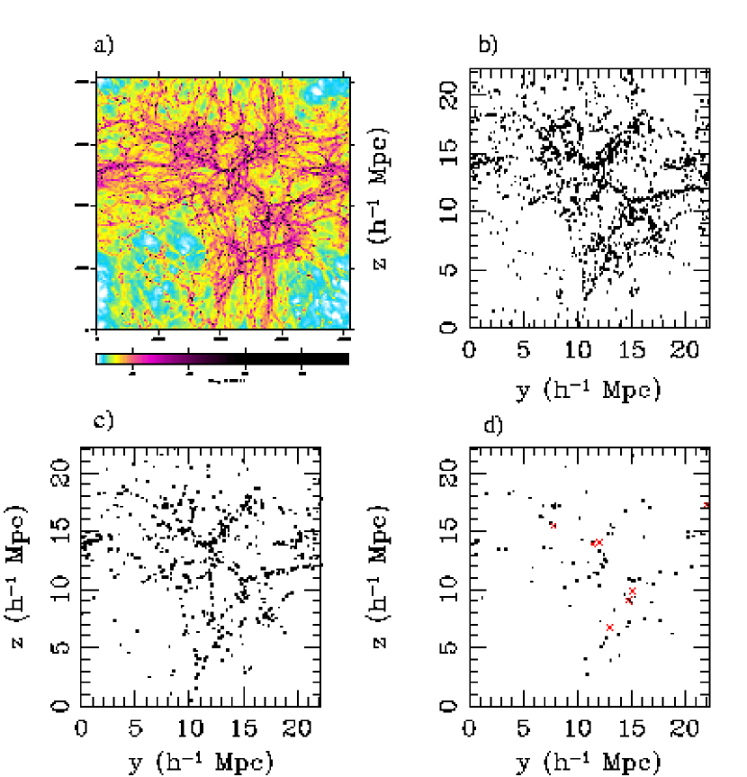
Figure 2.— (a) Column density map of Hi in the $22.222~{}h^{-3}$ Mpc³ volume projected along the $x$-axis on a 4096² pixel grid. Potential DLAs with $N_{\hbox{{\rm H}{\sc i}}}\;>\;10^{20.3}$ cm^-2 appear black. (b) Position of potential DLAs projected along the $x$-axis. (c) Position of the 651 galaxies that have a baryonic mass $M_{b}$ larger than the resolution $6.8\times 10^{9}$ M_⊙. (d) Position of the 100 most star-forming galaxies. The red crosses show the positions of the seven most star-forming galaxies.

The left panel of Figure 3 shows the mass probability distribution of all the resolved galaxies. The line shows the halo mass distribution obtained from the Press-Schechter (PS) formalism (Mo & White, 2002). The mean mass (logarithmic average) for all the 651 galaxies is shown ($\langle\log M_{h}(\hbox{M${}_{\odot}$})\rangle\;=\hbox{$11.57$}$). The right panel of Figure 3 shows the DLA halo mass distribution. The halo mass of a given DLA was obtained by matching the projected DLA positions (2-D) with those of the resolved halos. The projected distance distribution (between halos and DLAs) peaks at 8 kpc, with a tail to $\sim$20 kpc (physical units; see also Gardner et al. 2001), and there is very little ambiguity in identifying the halo of a DLA. Practically all the DLAs reside in halos with more than 64 dark matter particles. Note that, at $z=0$, the DLA distribution appears to be broadly peaked at around $V_{\rm rot}=110$ km s^-1 (Zwaan et al., 2005) and is even broader with respect to luminosity (Rosenberg & Schneider, 2003).

Figure 3.— Left: Halo mass (DM $+$ baryons) probability function $p(M)$ of all the SKID-identified galaxies with baryonic masses larger than the resolution $6.8\times 10^{9}$ M_⊙, corresponding to 64 SPH particles. For comparison, the curve is the dark matter mass function from the extended Press-Schechter formalism of Mo & White (2002) in this cosmology, scaled arbitrarily (i.e., not a fit). Right: DLA dark matter mass distribution, $p_{\rm DLA}(M)$ ($\propto\hbox{$\frac{\mathrm{d}N}{\mathrm{d}z\mathrm{d}\log M}$}$). This was found by matching the 2-D DLA positions with the nearest resolved halo. The shape of the distribution will not be constrained by the DLA-galaxy cross-correlation, but its first moment ($\langle\log M\rangle$) will be.

As mentioned, the purpose of this paper is to show that cross-correlation techniques will uniquely constrain the mean of this distribution, but will not constrain its shape. We refer the reader to Gardner et al. (2001) and Nagamine et al. (2004) for a detailed discussion of the DLA halo mass distribution in numerical simulations. Typically, in order to match the observed DLA statistics, they require an extrapolation of the DLA mass function below the mass resolution. Here we make no attempt to include halos smaller than our resolution since it would require putting in the appropriate cross-correlation signal by hand for halos smaller than our resolution.

3. Correlation functions in hierarchical models

In this section, we describe the fundamental clustering relations necessary to understand how one can determine the halo mass of DLAs.

A widely used statistic to measure the clustering of galaxies is the galaxy autocorrelation function $\xi_{\rm gg}(r)$. Similarly, one can define the cross-correlation $\xi_{\rm dg}$ between DLAs and galaxies from the conditional probability of finding a galaxy in a volume d$V$ at a distance $r=|\mathbf{r}_{1}-\mathbf{r}_{o}|$, given that there is a DLA at $\mathbf{r}_{o}$,

$$P(LBG|DLA)=\overline{n}_{u}(1+\xi_{\rm dg}(r))\mathrm{d}V,$$ (1)

where $n_{u}$ is the unconditional background galaxy density, i.e., the density when $\xi=0$.

At a given redshift, the autocorrelation and cross-correlation functions are related to the dark matter correlation function $\xi_{\rm DM}$ through the mean bias $\overline{b}(M)$ by

$$\xi_{\rm gg}(r) = \overline{b}^{2}(M_{\rm gal})\,\xi_{\rm DM}(r),$$ (2)

$$\xi_{\rm dg}(r) = \overline{b}(M_{\rm DLA})\,\overline{b}(M_{\rm gal})\,\xi_{\rm DM}(r),$$ (3)

where $M_{\rm gal}$ is the mean galaxy halo mass, $M_{\rm DLA}$ is the mean DLA halo mass, and $\overline{b}(M)$ is given by

$$\int_{M}^{\infty}p(M^{\prime})\;b(M^{\prime})\;\mathrm{d}M^{\prime}\,,$$ (4)

where $p(M)$ is the halo mass probability distribution and $b(M)$ is the bias function, which can be computed using the extended PS formalism (e.g., Mo et al., 1993; Mo & White, 2002). Thus, from equations 2–3, if both $\xi_{\rm dg}$ and $\xi_{\rm gg}$ are power laws $(\xi\propto r^{\gamma})$ with the same slope $\gamma$, the amplitude ratio of the cross- to autocorrelation is a measurement of the bias ratio $\overline{b}(M_{\rm DLA})/\overline{b}(M_{\rm gal})$, from which one can infer the halo masses $M_{\rm DLA}/M_{\rm gal}$. The details are presented in section 4.2. Briefly, given that $b(M)$ is a monotonic increasing function of $M$, if $\xi_{\rm dg}$ is greater (smaller) than $\xi_{\rm gg}$, then the halos of DLAs are more (less) massive than those of the galaxies.

In the remainder of this work, we use only projected correlation functions, $w(r_{\theta})$, where $r_{\theta}=D_{A}(1+z)\theta$ in comoving Mpc, where $D_{A}$ is the angular diameter distance. This is necessary since (1) the gas column density distribution is a 2-D quantity, and (2) this corresponds to the situation when one relies on photometric redshifts (e.g., Bouché & Lowenthal, 2003, BL04). Projected correlation functions $w(r_{\theta})$ is directly related to spatial correlation functions $\xi(r)$ if the selection function is known. Following Phillipps et al. (1978) and Budavári et al. (2003), the projected autocorrelation function, $w_{\rm gg}$, of galaxies with a redshift distribution ${\mathrm{d}N}/{\mathrm{d}z}$ is

$$w_{\rm gg}(r_{\theta}) = \int_{0}^{\infty}dz\left(\frac{\mathrm{d}N}{\mathrm{d}z}\right)^{2}g(z)^{-1}\times(f(z)\theta)^{1-\gamma}\;r_{0}^{\gamma}\;H_{\gamma}\;,$$ (5)

$$= (r_{\theta})^{1-\gamma}\;r_{\rm 0,gg}^{\gamma}\;H_{\gamma}\int_{0}^{\infty}dl\left(\frac{\mathrm{d}N}{\mathrm{d}l}\right)^{2}\,,$$

where ${\mathrm{d}N}/{\mathrm{d}l}$ is the galaxy redshift distribution in physical units, $f(z)=D_{A}(1+z)$ is the comoving line-of-sight distance, $g(z)=\mathrm{d}r/\mathrm{d}z=c/H(z)$, and $H_{\gamma}=\hbox{${\Gamma({1}/{2})\Gamma([{\gamma-1}]/{2})}/{\Gamma({\gamma}/{2})}$}$ (see Appendix A). The projected cross-correlation $w_{\rm dg}$ between a given absorber at a given redshift and the galaxies (with a distribution ${\mathrm{d}N}/{\mathrm{d}z}$) is

$$w_{\rm dg}(r_{\theta}) = \int\hbox{$\frac{\mathrm{d}N}{\mathrm{d}l}$}\ \xi(\sqrt{r_{\theta}^{2}+l^{2}})\,\mathrm{d}l\,.$$ (6)

For galaxies distributed in a top-hat redshift distribution ${\mathrm{d}N}{\mathrm{d}l}$ of width $W_{z}$ [normalized such that $\int({\mathrm{d}N}{\mathrm{d}l})\mathrm{d}l=1$], as in the case here, Equations 5 and 6 imply that the amplitudes of both $w_{\rm dg}(r_{\theta})$ and $w_{\rm dg}(r_{\theta})$ are inversely proportional to $W_{z}$ (see Appendix A for the derivations):

$$w_{\rm gg}(r_{\theta}) \simeq (r_{\theta})^{1-\gamma}\;r_{\rm 0,gg}^{\gamma}\;H_{\gamma}\times\left(\frac{1}{W_{z}}\right)^{2}\;W_{z}\,,$$ (7)

$$w_{\rm dg}(r_{\theta}) \simeq (r_{\theta})^{1-\gamma}\;r_{\rm 0,dg}^{\gamma}\;H_{\gamma}\times\frac{1}{W_{z}}\,.$$ (8)

Therefore, the ratio of the amplitudes of the two projected correlation functions $w_{\rm dg}$ to $w_{\rm gg}$ is simply $(r_{\rm 0,dg}/r_{\rm 0,gg})^{\gamma}$, or the bias ratio $\overline{b}(M_{\rm DLA})/\overline{b}(M_{\rm gal})$, from which we infer the mean DLA halo mass, regardless of the redshift distribution. This is an important result for surveys that rely on photometric redshifts: the ratio of the projected correlations is a true measure of the bias ratio, regardless of contamination or uncertainty in the actual redshift distribution, provided that the same galaxies are used for $w_{\rm dg}$ and $w_{\rm gg}$.

4. Results

In section 4.1, we quantify the amplitude of the DLA-galaxy cross-correlation relative to the galaxy-galaxy autocorrelation in the SPH simulations. We show how to invert the cross-correlation results into a mass constraint in section 4.2. We show that this method is independent of the galaxy sample that one uses (§ 4.3). Finally, we compare these results to observational results in section 4.4.

4.1. DLA-Galaxy Cross-Correlation

The filled circles in Figure 4 show the DLA-galaxy cross-correlation $w_{\rm dg}$ using the entire sample of 115,000 DLAs and the 651 resolved galaxies. We computed $w_{\rm dg}(r_{\theta})$ with the estimator

$$1+w_{\rm dg}(r_{\theta}) = \left\langle\frac{N_{\rm obs}(r_{\theta})}{N_{\rm exp}(r_{\theta})}\right\rangle,$$ (9)

where $N_{\rm obs}(r_{\theta})$ is the observed number of galaxies between $r_{\theta}-dr/2$ and $r_{\theta}+\mathrm{d}r/2$ from a DLA and $N_{\rm exp}(r_{\theta})$ is the expected number of galaxies if they were uniformly distributed, i.e., $N_{\rm exp}(r_{\theta})=2\pi r_{\theta}\Sigma_{g}\mathrm{d}r$ where $\Sigma_{g}$ is the galaxy surface density. $\langle\rangle$ denotes the average over the number of selected DLAs ($N_{\rm DLA}$). In counting the pairs, we took into account the periodic boundary conditions of the simulations.

Figure 4.— Filled circles show the projected DLA-galaxy cross-correlation $w_{\rm dg}(r_{\theta})$ at $z=3$ in this $22.222~{}h^{-3}$ Mpc³ simulation. The solid triangles show the projected autocorrelation $w_{\rm gg}(r_{\theta})$ (offset by 0.03dex in the $x$–axis for clarity). The full sample of 115,000 DLAs and 651 resolved galaxies was used. The amplitude ratio $a=\hbox{$0.73\pm 0.08$}$, which is $w_{\rm dg}/w_{\rm gg}$, is found by fitting $w_{\rm dg}$ to the model $\hat{w}_{\rm dg}=a\;\hat{w}_{\rm gg}$, where $\hat{w}_{\rm gg}$ is the fit to the galaxy-galaxy autocorrelation (dashed line). The small panel shows the $1\sigma$ range (vertical lines) of the $\chi^{2}$ distribution (solid line). An integral constraint of $C=0.04$ was used.

There are several reasons not to use other estimators such as the Landy & Szalay (1993, LS) estimator. First, we want to duplicate as closely as possible the method (and estimator) used in the observations of Bouché & Lowenthal (2003) and BL04. But, more importantly, the LS estimator is symmetric under the exchange of the galaxies with the absorbers, whereas here and for the observations of BL04, the symmetry is broken. This is due to the absorber redshift being well known, while galaxies have photometric redshifts with larger uncertainties and, therefore, are distributed along the line of sight. This broken symmetry is also fundamental in the derivation of equations 5–6. Had we used spectroscopic redshifts and $\xi(r)$ instead of $w(r_{\theta})$, the LS estimator would be superior.

Given that we use the galaxy surface density $\Sigma_{g}$ to estimate the unconditional galaxy density (see eq. 1), the integral of $\Sigma_{g}(1+w_{\rm dg})$ over the survey area $A$ will be equal to the total number of galaxies, i.e., $\int_{A}\Sigma_{g}(1+w_{\rm dg})\mathrm{d}A=N_{g}$. As a consequence, $\int\Sigma_{g}\;w_{\rm dg}\;\mathrm{d}A=0$, and the correlation will be negative on the largest scales, i.e., biased low. This is the known “integral constraint”. In the case of our $22.222~{}h^{-2}$ Mpc² survey geometry, we estimated the integral constraint to be $C=0.04$, or 2% of the cross-correlation strength at 1 $h^{-1}$ Mpc. We added $C$ to $w_{\rm dg}$ estimated from equation 9.

The uncertainty to $w_{\rm dg}$, $\sigma_{w}$, has two terms, the Poisson noise and the clustering variance (see Eisenstein, 2003, and references therein; Appendix B). In Appendix B, we show that $\sigma_{w}$ is proportional to $1/\sqrt{N_{\rm DLA}}$ (eq. B11).

There are several ways to compute $\sigma_{w}$ in practice. The proper way to compute $\sigma_{w}$ would be to resample the DLAs, since this would include the uncertainty due to the finite the number of lines of sight. However, this is valid for independent lines of sight, as in the case of an observational sample (provided that $N_{\rm DLA}$ is large, say greater than $10$), and will not be correct here given that we have only one simulation and that we have to use the same galaxies for each simulated line of sight. The uncertainty $\sigma_{w}$ must then reflect that we used only one realization of the large-scale structure. For this reason, we elected to use the jackknife estimator (Efron, 1982), i.e., by dividing the $22.222h^{-2}$ Mpc² area into nine equal parts and each time leaving one part out. This will accurately reflect the uncertainty in $w_{dg}$ due to the one large-scale structure used, but the signal-to-nois ratio (S/N$\equiv w_{\rm dg}/\sigma_{w}$) will not increase with $\sqrt{N_{\rm DLA}}$ as expected (Appendix B): it will saturate after a certain value of $N_{\rm DLA}$. We find that indeed the SNR saturates at $N_{\rm DLA}\simeq 40$ (not shown). This is a major difference from observational samples, where each field is independent. In that case, equation B11 applies and the S/N is proportional to $\sqrt{N_{\rm DLA}}$.

We computed the full covariance matrix from the $N_{\rm jack}=9$ realizations as

$${\rm COV}_{ij}=\frac{N_{\rm jack}-1}{N_{\rm jack}}\sum_{k=1}^{N_{\rm jack}}[w_{k}(r_{\theta_{i}})-\overline{w}(r_{\theta_{i}})]\cdot[w_{k}(r_{\theta_{j}})-\overline{w}(r_{\theta_{j}})]\;,$$ (10)

where $w_{k}$ is the $k$th measurement of the cross-correlation and $\overline{w}$ is the average of the $N_{\rm jack}$ measurements of the cross-correlation. The error bars in Figure 4 show the diagonal elements of the covariance matrix, i.e., $\sigma_{w}\equiv\sqrt{{\rm COV}_{ii}}$.

We computed the projected autocorrelation $w_{\rm gg}(r_{\theta})$ of the same simulated galaxies used for $w_{\rm dg}(r_{\theta})$ in a similar manner. We used the estimator shown in equation 9 to compute $w_{\rm gg}(r_{\theta})$, where $N_{\rm obs}(r)$ is now the number of galaxies between $r-\mathrm{d}r/2$ and $r+\mathrm{d}r/2$ from another galaxy. The open triangles in Figure 4 show the projected autocorrelation $w_{\rm gg}(r_{\theta})$ of the 651 galaxies.

We fitted the galaxy autocorrelation with a power law model (${\hat{w}}_{\rm gg}=A_{\rm gg}r_{\theta}^{\beta}$) by minimizing $\chi^{2}\propto[\mathbf{w}-\mathbf{\hat{w}}]^{T}\mathrm{COV}^{-1}[\mathbf{w}-\mathbf{\hat{w}}]$, where $\mathbf{w}$ and $\mathbf{\hat{w}}$ are the vector data and model, respectively, and ${\rm COV}^{-1}$ is the inverse of the covariance matrix. We used single value decomposition (SVD) techniques to invert the covariance matrix, ${\rm COV}$, since it is singular and the inversion is unstable (see discussion in Bernstein, 1994).

We then use that fit as a template to constrain the amplitude of $w_{\rm dg}$, i.e.,

$$\hat{w}_{\rm dg}=a\times\hat{w}_{\rm gg},$$ (11)

where $a$ is the amplitude ratio $A_{\rm dg}/A_{\rm gg}$ of the correlation functions. This assumes that the two correlation functions have the same slope (see § 3). This method also closely matches the method used by BL04 (see § 4.4 below) and makes comparison to those observations straightforward.

The solid line in Figure 4 shows the fit to $w_{\rm dg}$ using equation 11, where the best amplitude $a$ is

$$a=\hbox{$0.73\pm 0.08$}\,.$$ (12)

The top panel shows the $\chi^{2}(a)$ distribution with the $1\sigma$ range. In other words, the bias ratio $\overline{b}(M_{\rm DLA})/\overline{b}(M_{\rm gal})$ is $0.73\pm 0.08$. This can be converted into a correlation length for $w_{\rm dg}$ of $a^{1/1.8}\simeq 0.84$ times that of the galaxy autocorrelation, i.e., $r_{\rm 0,dg}\simeq 0.84\;r_{\rm 0,gg}$.

Several authors (e.g., Berlind & Weinberg, 2002; Berlind et al., 2003, and references therein) have shown that the small scales ($r\langle 1$ Mpc) of the correlation function are the scales sensitive to variations in the halo occupation number. At those scales, $\xi(r)$ is very susceptible to galaxy pairs that are in the same halo. Therefore, when we repeated our analysis with the six subsamples, we restricted ourselves to $r_{\theta}\,>\,1$ $h^{-1}$ Mpc. In this case, for the full sample, we find the amplitude ratio to be $a=0.70\pm 0.18$, in good agreement with equation 12.

The reader should not use these results (e.g., eq. 12), obtained with 651 galaxies and 115,000 DLAs, to scale the errors to smaller samples, because we use the same large-scale structure for all the 115,000 simulated DLAs. As mentioned earlier, the large-scale structure dominates the uncertainty at large $N_{\rm DLA}$, and this is seen in the fact that the S/N saturates after $N_{\rm DLA}\simeq 40$. We come back to this point at the end of § 4.4.

4.2. The Mass of DLA Halos from the Amplitude of $w_{\rm dg}$

Equation 12, i.e., the bias ratio $\overline{b}(M_{\rm DLA})/\overline{b}(M_{\rm gal})$, can be converted into a mean halo mass for DLAs if one knows the functional form of $b(M)$ and $M_{\rm gal}$. One can use the PS formalism (e.g., Mo & White, 2002) or the autocorrelation of several galaxy subsamples to constrain the shape of $b(M)$. We refer to these as the “theoretical method” and as the “empirical method,” respectively.

4.2.1 Theoretical Biases $b(M)$

One can compute the theoretical biases for any population (eq. 4) and predict the bias ratio a priori if the mass probability distribution $p(M)$ is known. Naturally, $p(M)$ is known in our simulation (Fig. 3). We show that the predicted bias ratio is well within the $1\sigma$ range of our results (eq. 12), demonstrating the reliability of the method.

Given that galaxies and the DLAs actually lie in halos of different masses, the theoretical biases are found from equation 4, i.e.,

$$\overline{b}_{\rm DLA}(>M) = \int_{M}^{\infty}p_{\rm DLA}(M^{\prime})\;b(M^{\prime})\;\mathrm{d}\log M^{\prime}\;,$$ (13)

$$\overline{b}_{\rm gal}(>M) = \int_{M}^{\infty}p_{\rm gal}(M^{\prime})\;b(M^{\prime})\;\mathrm{d}\log M^{\prime}\;,$$ (14)

where $p(M)$ is the appropriate mass distribution [$p(M)\equiv\frac{\mathrm{d}n}{\mathrm{d}\log M}$ normalized such that $\int p(M)\mathrm{d}\log M=1$] and $b(M)$ is the bias of halos of a given mass $M$. The bias function $b(M)$ is also a function of redshift $z$, i.e., $b(M,z)$, and can be computed at a given $z$ from the extended PS formalism (e.g., Mo & White, 2002). It is shown in Figgure 5 for $z=3$ on a linear-linear (left) and log-linear (right) plot.

Figure 5.— Left: The $z=3$ bias $b(M)$ as a function of halos of mass $M$ from the extended Press-Schechter theory, as in Mo & White (2002). Right: Same as left panel in $\log M$ space. In both panels, the dashed line is a linear fit to the curve over the mass range $\log M\sim 11.5$—$12.5$.

The mass distributions $p_{\rm DLA}$ and $p_{\rm gal}$ are shown in Figgure 3. Because $p(M)$ is bounded at some low-mass limit $M_{\rm min}$ (due to limited resolution or to observational selection), the mean bias $\overline{b}$ of a given galaxy sample is defined by $\overline{b}_{gal}=\overline{b}(>M_{\rm min})$.

The predicted biases $\overline{b}$ are shown in the left panel of Figure 6. The predicted biases $\overline{b}$ for the subsamples, the 651 galaxies, and the DLAs are represented by open squares, the filled square and the filled circle, respectively. From $\overline{b}$ for the 651 galaxies (filled square) and for DLAs (filled circle), the theoretical bias ratio $\overline{b}_{\rm DLA}/\overline{b}_{\rm gal}$ is found to be $0.771$, very close to the bias ratio measured from the clustering of galaxies around the DLAs (eq. 12).

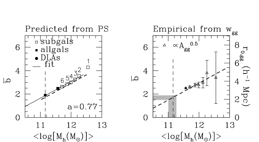
Figure 6.— Left: The symbols show the mean bias $\overline{b}$ as a function of the mean halo mass $\langle\log M_{h}\rangle$ for the DLAs (circle), full galaxy sample (filled square) and the subsamples (open squares), labeled 1–6. The bias is calculated using equations 13–14 and the distributions $p_{\rm DLA}$ and $p_{\rm gal}$ (shown in Fig. 1). From the filled symbols, the predicted bias ratio is found to be $0.771$. The solid line is a linear fit to the points and is 5% away from to the linear approximation (Fig. 5) shown by the thick dashed line. Right: Same as left panel, but using the empirical method (see text) instead of the mass distributions. The triangles show the mean bias for the different galaxy samples using $\overline{b}\propto\sqrt{A_{gg}}$ (eq. 2) where the normalization was adjusted to match the amplitude of the dashed line. The bias for the 651 galaxies is represented by the filled triangle. The open triangles show $\overline{b}$ for the subsamples. The right axis scale shows the corresponding correlation length $r_{0}$. For the DLAs, the shaded areas show the measured bias ratio $a=\hbox{$0.73\pm 0.08$}$ and the corresponding halo mass range $\langle\log M_{\rm DLA}(\hbox{M${}_{\odot}$})\rangle\;=\hbox{$11.13^{+0.13}_{-0.13}$}$ using the mean mass of the 651 resolved galaxies: $\langle\log M_{\rm gal}(\hbox{M${}_{\odot}$})\rangle\;=\hbox{$11.57$}$. In both panels, the vertical dashed line shows the “true” mean $\langle\log M_{\rm DLA}(\hbox{M${}_{\odot}$})\rangle=\hbox{$11.16$}$ obtained from the DLA mass distribution $p_{\rm DLA}(M)$ shown in Figure 3. Both panels are for $z=3$.

When the distributions $p(M)$ are not known, we can infer a mass ratio from the bias ratio using the approximation $b(M)=b_{0}+b_{1}\;\log M$, over a restricted mass range. In each panel in Figure 5, the dashed line shows such a linear fit over the mass range $\log M\sim 11$—$12.5$. Using this approximation, the mean bias $\overline{b}$ is given by

$$\overline{b}(\>M_{\rm min}) = \int_{M_{\rm min}}^{\infty}p(M^{\prime})\;b(M^{\prime})\;\mathrm{d}\log M^{\prime}$$ (15)

$$= b_{0}+b_{1}\;\int_{M_{\rm min}}^{\infty}p(M^{\prime})\;\log M^{\prime}\;\mathrm{d}\log M^{\prime}$$

$$= b_{0}+b_{1}\;\langle\log M\rangle\;,$$

where $\langle\log M\rangle$ is the first moment of the distribution $p(M)$. Thus, the mean bias for the galaxies and the DLAs are $\overline{b}_{\rm gal}=b(\langle\log M_{\rm gal}\rangle)$, and $\overline{b}_{\rm DLA}=b(\langle\log M_{\rm DLA}\rangle)$, respectively, where $\langle\rangle$ denote the first moment of the appropriate mass distribution.

In Figure 6 (left) the solid line is a linear fit to the theoretical biases $\overline{b}(\langle\log M\rangle)$, and is 5% away (in amplitude) from the linear approximation (eq. 15) shown by the thick dashed line. The vertical dashed line indicates the mean DLA halo mass $\langle\log M_{\rm DLA}\rangle$ that is found from the first moment of the mass distribution in Figure 3. This shows that using a linear approximation of $b(M)$ is equivalent to using the bias function $b(M)$ from Mo & White (2002), provided that the DLA-galaxy mass ratio is not larger than a decade. Indeed, the 5% difference in amplitude cancels out when taking the bias ratio.

4.2.2 Empirical Method for $b(M)$

To infer $\langle\log M_{\rm DLA}\rangle$ from equation 12 or from observations, one needs to find the coefficients $b_{0}$ and $b_{1}$. To do so, one can either use the PS formalism (Mo & White, 2002) or use the fact that $\overline{b}$ is proportional to $\sqrt{A_{\rm gg}}$ (eq. 2), where $A_{\rm gg}$ is measured for each of the galaxy subsamples covering the mass range $\log M\sim 11.5$—$12.5$. Figure 6 (right) illustrates this point. The thick dashed line is again the linear approximation shown in Figure 5. The open (filled) triangles show the mean biases $\overline{b}$ of the subsamples (full sample) assuming that $\overline{b}\propto\sqrt{A_{\rm gg}}$ (eq. 2). The normalization is set to match the dashed line, and is not relevant, since we measure a ratio of two biases. This shows that one can use either the PS formalism (Mo & White, 2002) or use $\sqrt{A_{\rm gg}}$ to find the coefficients $b_{0}$ and $b_{1}$.

In the case where the autocorrelation length $r_{\rm 0,gg}$ has been determined, one can use the right $y$–axis scale of Figure 6 the infer the DLA halo mass from the measured bias ratio.

4.2.3 The Mean DLA Halo Mass

To actually determine $\langle\log M_{\rm DLA}\rangle$ from our cross-correlation result (eq. 12), we used (1) the linear approximation to the PS bias (Fig. 6, thick dashed line), and (2) $\langle\log M_{\rm gal}\rangle=\hbox{$11.57$}$ for the 651 galaxies. We infer a mean DLA halo mass of $\langle\log M_{\rm DLA}\rangle=\hbox{$11.13^{+0.13}_{-0.13}$}$, shown by the vertical shaded area on the right panel of Figure 6. Our cross-correlation result (eq. 12) is shown by the horizontal shaded area. The “true” DLA mass derived from $p_{\rm DLA}$ (Fig. 3) and equation 13 is shown by the vertical dashed line at $\log M_{\rm DLA}=\hbox{$11.16$}$. Similarly, using fits to $b(M)$ in linear space (Fig. 5, left), we infer $\langle M_{\rm DLA}\rangle=\hbox{$2.12^{+2.96}_{-2.0}\times 10^{11}$}$ M_⊙, close to “true” mean $1/N_{\rm DLA}\sum_{i}M_{\rm DLA,i}=\hbox{$3.94\times 10^{11}$}$ M_⊙.

In summary, the amplitude of $w_{\rm dg}$ relative to $w_{\rm gg}$, $a=\hbox{$0.73\pm 0.08$}$ (eq. 12), measured in this simulation implies that DLAs have halos of (logarithmically) averaged mass

$$\langle\log M_{\rm DLA}(\hbox{M${}_{\odot}$})\rangle\;=\hbox{$11.13^{+0.13}_{-0.13}$}\;,$$ (16)

close to the true $11.16$. This shows that the cross-correlation technique uniquely constrain the mean of the halo mass distribution, despite the fact that DLAs occupy a range of halo masses and some halos contain multiple galaxies and multiple DLA systems. In § 4.3, we show that the technique is reliable in the sense that it will lead to the same answer regardless of the galaxy sample used.

From the right panel of Figure 6, we can now predict the cross-correlation strength for real $z=3$ LBGs, which have a correlation length of $r_{\rm 0,gg}\simeq 4$ Mpc (e.g., ASSP03; Adelberger et al., 2004), corresponding to a halo mass of $M_{\rm h}\simeq 10^{12}$ M_⊙. From the figure, one expects that the correlation ratio or the bias ratio is $\sim 1.75/3=0.58$, and thus the DLA-LBG cross-correlation would have a correlation length $r_{\rm 0,dg}=4\times(0.58)^{1/1.6}\simeq\hbox{$2.85$}$ Mpc.

Potential systematic errors include the few massive halos ($M_{h}>10^{13}$ M_⊙) that are missed due to the limited volume ($22.222~{}h^{-3}$ Mpc³) of our simulation. However, since DLAs are cross section selected these few massive halos are too scarce to change the mean $\langle\log M_{\rm DLA}\rangle$ of the DLA mass probability distribution (Fig. 3, right). Naturally, if there were such massive halos in our simulations, the amplitude of the cross-correlation would be different. We address this point in a general way in § 4.3 and show that the derived $\langle\log M_{\rm DLA}\rangle$ is independent of the galaxy sample used.

Our treatment of feedback is limited to energy injection of supernovae, and thus does not treat phenomena like winds. Nagamine et al. (2004) included winds in similar simulations and showed that the DLA abundance decreases with increasing wind strength, but the mean DLA halo mass will be shifted towards higher mass in the presence of winds. Nagamine et al. (2004) also showed that the DLA abundance (extrapolated to $10^{8}$ M_⊙, i.e., below the resolution limit, using the PS formalism) also decreases with increasing resolution, but again, the mean DLA halo mass will be shifted toward higher mass in higher resolution runs.

Given that (1) a fraction of DLAs are expected to arise in halos below our mass resolution of $M_{h}\gtrsim 5.2\times 10^{10}$ M_⊙ and (2) our total DLA abundance extrapolated to $10^{8}$ M_⊙, as in Nagamine et al. (2004), over-predicts the observed DLA abundance, equation 16 is an upper limit. Furthermore, given the results of Nagamine et al. (2004) showed that both winds and better resolution increase the mean DLA halo mass, we conclude that a simulation with SNe winds and with a better mass resolution would lower our mean DLA mass. Reading from Figure 5 in Nagamine et al. (2004), we estimate that $\langle\log M_{\rm DLA}\rangle$ is $\sim 10.6$ in their high-resolution run with strong winds, or a factor of $\sim 5$ smaller than here. Thus, equation 16 is an upper limit.

4.3. The Cross-Correlation Is Independent of the Galaxy Sample

From equations 2 and 3, we expect the relative amplitude $a$ to vary as a function of the halo mass of the galaxy sample $M_{\rm h}$. We therefore performed the same cross-correlation calculations for each of the six subsamples presented in § 2 (see also Fig. 1), and ask the question, is the inferred $\langle M_{\rm DLA}\rangle$ the same in each case? We restricted ourselves to scales $r_{\theta}\,>\,1$ $h^{-1}$ Mpc (from the discussion in § 4.1).

Figure 7 shows the measured amplitude or bias ratio $a$ for each of the subsamples. The amplitude ratio $a$ for the subsamples (full sample) is represented by the open squares (filled circle) with solid error bars. The filled circle with dotted error bars represents the full sample shown in Figure 4 from which we inferred $a=\hbox{$0.73\pm 0.08$}$ and $\langle\log M_{\rm DLA}\rangle=\hbox{$11.13^{+0.13}_{-0.13}$}$. As expected, $a$ increases with larger subsamples, or with decreasing galaxy halo mass $M_{\rm h}$.

Figure 7.— DLA-LBG cross- to autocorrelation amplitude ratio, $a$ (defined in eq. 11), as a function of the mean galaxy halo mass $\langle\log M_{h}\rangle$ using the full DLA sample of $\sim 115,000$ lines of sight. Note that $a$ is also $\overline{b}(M_{\rm DLA})/\overline{b}(M_{\rm gal})$. Each of the subsamples (see Fig. 1) is labeled 1–6. The filled circle with solid error bars shows $a$ for the entire sample of 651 galaxies and 115,000 DLAs. The filled circle with dotted error bars (offset along the $x$-axis) shows $a$ fitted over all scales for the entire sample of 651 galaxies and 115,000 DLAs from which we infer a mean DLA halo mass of $\langle\log M_{\rm DLA}\rangle=\hbox{$11.13^{+0.13}_{-0.13}$}$. For this mass, the expected amplitude ratio $a$ for the six subsamples is shown by the solid line. The expected $a$ follows closely the values found for the subsamples, showing that one will get the same DLA halo mass for any galaxy subsample, as long as the same galaxies are used for $w_{\rm gg}$ and $w_{\rm dg}$, i.e., that the method is reliable and self-consistent. For comparison, the dashed lines show the expected $a$ if the mean DLA halo mass $\langle\log M_{\rm DLA}\rangle$ were 10.5, 11.5, and 12 (from bottom to top) instead.

For the method to be self-consistent, the derived DLA halo mass $\langle\log M_{\rm DLA}\rangle$ should be the same for all the subsamples. Given equation 15, $\langle\log M_{\rm DLA}\rangle=11.13$ determined in § 4.2, and a mean galaxy halo mass $\langle\log M_{h}\rangle$, we can predict the bias ratio $a$. The solid line in Figure 7 represents this prediction. One sees that the measured bias ratio for the subsamples (open squares) follow the expected bias ratio (solid line). For comparison, the dashed lines show the expected amplitude ratios $a$ if DLAs were in halos of mean mass $\langle\log M_{\rm DLA}\rangle=10.5$, 11.5, and 12 (from bottom to top) instead of the inferred $\langle\log M_{\rm DLA}\rangle=11.13$.

We conclude that the method is reliable and self-consistent, i.e., the mass $\langle\log M_{\rm DLA}\rangle$ is independent of the galaxy sample used, that the clustering statistics of DLAs with galaxies can be used to infer their mass, and that large observational samples will shed new light on their nature. A direct observational measure of the relative amplitude $a$ (J. Cooke 2005, private communication), will show whether or not DLAs are massive disks ($10^{12}~{}\hbox{M${}_{\odot}$}$) as proposed by Wolfe et al. (1986, 1995) and Prochaska & Wolfe (1997b).

4.4. Comparison to Observations

In this section, we first briefly review past and recent observations of clustering between galaxies and DLAs (§ 4.4.1). We then (§ 4.4.2) focus on comparing the simulated DLA-LBG cross-correlation to the observational results of BL04, in a meaningful way, i.e., with a sample of similar size.

4.4.1 Observations of the DLA-Galaxy Cross-Correlation at $z=3$

Early attempts to detect diffuse Ly$\alpha$ emission from DLAs at $z>2$ using deep narrow band imaging (Lowenthal et al., 1995) did not reveal the absorber but unveiled a few companion Ly$\alpha$ emitters (Lowenthal et al., 1991), hinting at the clustering of galaxies around DLAs. This prompted Wolfe (1993) to calculate the two-point correlation function at $\langle z\rangle=2.6$ and to conclude that, indeed, Ly$\alpha$ emitters are clustered near DLAs at the $99$% or greater confidence level. Some recent Ly$\alpha$ searches have succeeded in unveiling the absorber (e.g., Fynbo et al., 1999).

Francis & Hewett (1993) reported the discovery of super-clustering of sub-DLAs at $z\sim 2.4$ and $2.9$: a total of four Hi clouds are seen in a QSO pair separated by 8′, each being at the same velocity. Recent results from narrow-band imaging of the Francis & Hewett field show that spectroscopically confirmed Ly$\alpha$ emitters are clustered at the redshift of the strongest Hi cloud at $z=2.9$ ($\log N_{\hbox{{\rm H}{\sc i}}}=20.9$) towards Q2138-4427 (Fynbo et al., 2003). Roche et al. (2000) identified eight Ly$\alpha$ emitting galaxies near the DLA at $z=2.3$ towards PHL 957 in addition to the previously discovered Coup Fourré galaxy (Lowenthal et al., 1991), implying the presence of a group, filament, or proto-cluster associated with the DLA. Other evidence of clustering includes the work of Ellison et al. (2001), who found that the DLA at $z_{\rm abs}=3.37$ towards Q0201+1120 is part of a concentration of matter that includes at least four galaxies (including the DLA) over transverse scales greater than $5~{}h^{-1}$ Mpc, and of D’Odorico et al. (2002) who showed that out of 10 DLAs in QSO pairs, five are matching systems within 1000 km s^-1. They concluded that this result indicates a highly significant over-density of strong absorption systems over separation lengths from $\sim 1$ to $8~{}h^{-1}$ Mpc.

Gawiser et al. (2001) studied the cross-correlation of LBGs around one $z\sim 4$ DLA. Probably due to the high redshift of their DLA, Gawiser et al. (2001) found that $w_{\rm dg}(r_{\theta})$ is consistent with 0, i.e., they found that the distribution of the eight galaxies in that field (with spectroscopic redshifts) is indistinguishable from a random distribution. Their data did not allow them to put limits on the amplitude of $w_{\rm dg}$.

Recently, ASSP03 found a lack of galaxies near four DLAs and concluded that the DLA-LBG cross-correlation is significantly weaker than the LBG-LBG autocorrelation at the 90% confidence level. They found two LBGs within $r_{\theta}=5.7$ $h^{-1}$ Mpc and within $W_{z}\langle 0.0125$ ($\sim 8$ $h^{-1}$ Mpc) whereas $\sim 6$ were expected if the cross-correlation has the same amplitude as the galaxy autocorrelation. Because of the field of view available, both Gawiser et al. (2001) and ASSP03 were not sensitive to scales larger than $r_{\theta}\sim 5~{}h^{-1}$ Mpc, which is important since the relevant scales to measure the DLA-LBG cross-correlation extend up to $r_{\theta}\sim 10~{}h^{-1}$ Mpc.

However, the results of ASSP03 can be used to put an upper limit on $w_{\rm dg}/w_{\rm gg}$ through the following steps: First, note that the two galaxies (in $N_{\rm DLAs}=4$ fields) observed by ASSP03 give

$$\langle N_{\rm obs}\rangle=2/4=0.5=\langle N_{\rm exp}\rangle(1+\overline{\xi}_{\rm dg})\,,$$ (17)

and the six galaxies expected if $\overline{\xi}_{\rm dg}=\overline{\xi}_{\rm gg}$ give $\langle N_{\rm exp}\rangle(1+\overline{\xi}_{\rm gg})=6/4$, where $\overline{\xi}$ is the volume average of the correlation function. Second, for the LBG autocorrelation published in ASSP03, we find $\overline{\xi}_{\rm gg}\simeq 1.1$, averaged over a sphere centered on the DLAs with an effective radius of $\sim 6$ $h^{-1}$ Mpc, i.e., with the same volume as the cylindrical cell used by ASSP03. Thus, the expected number of galaxies per DLA field is $\langle N_{\rm exp}\rangle=0.68$ if $\overline{\xi}_{\rm dg}=0$, and the total number of galaxies is $4\times\langle N_{\rm exp}\rangle=2.85$. Clearly their measurement of two galaxies is consistent with no cross-correlation. From equation 17, we can infer that $1+\overline{\xi}_{\rm dg}=0.7$ using $\langle N_{\rm exp}\rangle=0.68$. Third, the uncertainty to $\overline{\xi}_{\rm dg}$, $\sigma_{\xi}$, can be estimated using the results shown in Appendix B. The variance $V(\xi)=\sigma_{\xi}^{2}$ is made of two terms, the shot noise variance $V_{\rm sn}$ and the clustering variance $V_{\rm cl}$. The shot noise variance to $\langle N_{\rm obs}\rangle$ is $V(\langle N_{\rm obs}\rangle)_{\rm sn}=\langle N_{\rm obs}\rangle=0.5$ (eq. B2). The two-point clustering variance (eq. B6) is simply $\overline{N}^{2}(A\overline{\xi}_{\rm gg})=\overline{N}^{2}(2.50)$ where $A=J_{2}/K_{1}=2.28$. The three-point clustering variance (eq. B7) is $\sim 0$ since $\xi_{\rm dg}\simeq 0$. Finally, from equation B11, $\sigma_{\xi}=\frac{1}{\sqrt{4}}\frac{1}{\sqrt{2.85/4}}\sqrt{(1+\frac{2.5}{0.7})}\sqrt{0.7}\simeq 1.06$, and a 1-$\sigma$ (2-$\sigma$) upper limit to $\overline{\xi}_{\rm dg}$ is $\overline{\xi}_{\rm dg}+1(2)\sigma_{\xi}=-0.3+1.06(2.12)=0.76(1.82)$. Since $\overline{\xi}_{\rm gg}=1.1$, the 1-$\sigma$ (2-$\sigma$) upper limit to the amplitude ratio is $\overline{\xi}_{\rm dg}/\overline{\xi}_{\rm gg}\;\lesssim\;0.70(1.65)$, respectively. This rough calculation is quite consistent with Adelberger’s results where it was found that $\xi_{\rm dg}<\xi_{\rm gg}$ at the 90%  confidence level using Monte Carlo simulations.

Given that the relevant scales to measure the DLA-LBG cross-correlation extend up to $r_{\theta}\sim 10$ $h^{-1}$ Mpc, Bouché & Lowenthal (2003) were able to first detect and measure a DLA-LBG cross-correlation signal (BL04) using the wide-field ($0.35$ deg² or $\sim 40^{2}$ Mpc² comoving at redshift $z=3$) imager MOSAIC on the Kitt Peak 4m telescope. Bouché & Lowenthal (2003) showed that there was an over-density of LBGs by a factor of $\sim 3$ (with 95% confidence) around the $z_{\rm abs}\simeq 3$ DLA towards the quasar APM 08279+5255 ($z_{\rm em}=3.91$) on scales $2.5<r_{\theta}<5$ $h^{-1}$ Mpc. Extending the results of Bouché & Lowenthal (2003) to three $z\sim 3$ DLA fields, BL04 probed the DLA-LBG cross-correlation on scales $r_{\theta}\sim 5$–$20$ $h^{-1}$ Mpc and found (1) a DLA-LBG cross-correlation with a relative amplitude $w_{\rm dg}=(1.62\pm 1.32)\,w_{\rm gg}$ that is greater than zero at the $\sim 95$% confidence level, and (2) that $w_{\rm dg}$ is most significant on scales 5–10 $h^{-1}$ Mpc. In other words, DLAs are clustered with LBGs, but unfortunately the sample size did not allow BL04 to test whether $a$ is greater or smaller than 1. Soon, the ongoing survey of 9 $z\simeq 3$ DLAs of Cooke et al. (2005) will triple the sample of BL04.

In a slightly different context, Bouché et al. (2004) applied successfully the technique presented here to 212 $z\simeq 0.5$ Mg ii systems (of which 50% are expected to be DLAs) using luminous red galaxies (LRGs) in the Sloan Digital Sky Survey Data Release 1. They found that the Mg ii–LRG cross-correlation has an amplitude $0.67\pm 0.09$ times that of the LRG–LRG autocorrelation, over comoving scales up to $r_{\theta}=13$ $h^{-1}$ Mpc. Since LRGs have halo-masses greater than $3.5\times 10^{12}$ M_⊙ for $M_{R}\!\lesssim\!-21$, this relative amplitude implies that the Mg ii host galaxies have halo masses greater than $\sim 2$–$8\times 10^{11}$ M_⊙. These results show how powerful the cross-correlation technique is.

To summarize the current observational situation on the $z=3$ DLA-LBG cross-correlation, ASSP03 finds that the amplitude ratio is $\overline{\xi}_{\rm dg}/\overline{\xi}_{\rm gg}\;\lesssim\;0.70$, and BL04 finds that $\overline{\xi}_{\rm dg}/\overline{\xi}_{\rm gg}\;\gtrsim\;0.30$, both at the 1-$\sigma$ level. Using Monte Carlo simulations, ASSP03 finds $\overline{\xi}_{\rm dg}/\overline{\xi}_{\rm gg}\;<\;1.0$, at the 90% confidence level, and BL04 finds $\overline{\xi}_{\rm dg}/\overline{\xi}_{\rm gg}\;>\;0.0$, at the 95% confidence level. The DLA halo mass range allowed by these observations is still large: it covers $\log M_{\rm DLA}\sim{10}$–${12}$ M_⊙.

4.4.2 Simulation of Present Observations: $w_{\rm dg}$ with Small Samples

There are many significant differences between the observational sample of BL04 and the present simulated one. First, the shape of the volume is very different: the survey volume of BL04 is $40\times 40\times 100~{}h^{-3}$ Mpc³ (comoving), while these simulations are $22.222~{}h^{-1}$ Mpc (comoving) on a side. Given that the survey of BL04 contains about 80–120 LBGs per field, their observed LBG number density corresponds to about seven galaxies per $22.222~{}h^{-3}$ Mpc³. Naturally, seven galaxies are not a fair sample of the LBG luminosity function. This is an inherent problem due to the size of the simulation, rendering the comparison between the observed and the simulated cross-correlation difficult. Second, as mentioned in § 2, the simulated LBGs are selected according to their SFR, while the observed LBGs are color selected. Third, the same galaxies are used for every simulated line of sight. These differences limit our ability to perform a direct comparison to observations.

With these caveats in mind, we can repeat our analysis of section 4.2 in the limit of small $N_{\rm DLA}$ and with similar galaxy number densities. Because, to first order, $\sigma_{w}\propto(\sqrt{N_{\rm DLA}N_{\rm gal}})^{-1}$ (eq. B11), a sample made of 10 DLAs and 25 galaxies per $22.222^{2}~{}h^{-2}$ Mpc² “field” is expected to have similar errors to the sample of BL04 made of three DLAs and 100 galaxies per $40^{2}~{}h^{-2}$ Mpc² field. As for the full sample, we restricted ourselves to scales $r_{\theta}\;>\;1$ $h^{-1}$ Mpc, which also corresponds to the most relevant scales 5–10 $h^{-1}$ Mpc of the observations of BL04. We find that the relative amplitude of the cross-correlation with 10 lines of sight and 25 galaxies is $a=0.77\pm 0.53$, whereas BL04 found $a=1.62\pm 1.32$, i.e., both with the same S/N.

This confirms the results of BL04. More importantly, one can now use the result for this sample made of 10 DLAs and 25 galaxies (with a surface density $\Sigma_{\rm g}\sim 0.05$ Mpc^-2) as a benchmark to predict the S/N for the larger samples of future observations, given that the S/N will be proportional to $\sqrt{N_{\rm gal}N_{\rm DLA}}$ (eq. B11).

5. Conclusions

Motivated by the fact that (1) the amplitude of the cross-correlation is a measurement of the mean DLA halo mass and (2) observational constraints (Gawiser et al. 2001; ASSP03; BL04; J. Cooke et al. 2005, private communication) are reaching a turning point and the DLA halo masses are starting to be constrained, we tested the cross-correlation technique using TreeSPH cosmological simulations. The method uses the ratio of the cross-correlation between DLAs and high-redshift galaxies to the autocorrelation of the galaxies themselves, which is (in linear theory) the ratio of their bias factor, to infer the mean DLA halo mass.

In a TreeSPH simulation (Katz et al., 1996a) parallelized by Davé et al. (1997) with $128^{3}$ particles in a volume 22.222³ $h^{-3}$ Mpc³ (comoving), we find the following:

1. Scales $r_{\theta}>1$–15 $h^{-1}$ Mpc are the most relevant scales to constrain the mean DLA halo mass using the projected cross-correlation $w_{\rm dg}(r_{\theta})$.

2. The DLA-galaxy cross-correlation has an amplitude $w_{\rm dg}=(\hbox{$0.73\pm 0.08$})\;w_{\rm gg},$ close to the predicted value of $0.771$ using the Mo & White (2002) formalism.

3. The inferred mean DLA halo mass is

   $$\langle\log M_{\rm DLA}(\hbox{M${}_{\odot}$})\rangle\;=\hbox{$11.13^{+0.13}_{-0.13}$}\;,$$ (18)

   in excellent agreement with the true values of the simulations, i.e., $\langle\log M_{\rm DLA}\rangle=\hbox{$11.16$}$. Thus, even though DLAs and galaxies occupy a broad range of halos with massive halos containing multiple galaxies with DLAs, the cross-correlation technique yields the first moment of the DLA halo mass distribution.

4. If we consider subsets of the simulated galaxies with higher star-formation rates (representing LBGs), the cross-correlation technique is self-consistent, i.e., the DLA mass inferred from the ratio of the correlation functions does not depend on the galaxy sample used. This demonstrates the reliability of the method.

5. For real $z=3$ LBGs with a correlation length $r_{\rm 0,gg}\simeq 4$ $h^{-1}$ Mpc (ASSP03; Adelberger et al., 2004), our results imply that the DLA-LBG cross-correlation is expected to have a correlation length $r_{\rm 0,dg}\;\simeq\hbox{$2.85$}~{}h^{-1}$ Mpc.

6. With small samples (with 10 lines of sight and 25 galaxies) matching the statistics of BL04, the relative amplitude of the cross-correlation is $a=0.77\pm 0.53$, i.e., with a signal-to-noise ratio (S/N$\sim 1.3$–$1.5$) comparable to BL04, where they found $a=1.62\pm 1.32$.

In short, the cross-correlation between galaxies and DLAs is a powerful and self-consistent technique to constrain the mean mass of DLAs, and we have demonstrated its reliability. Given the resolution limits of the simulation used here ($M_{h}\gtrsim 5.2\times 10^{10}$ M_⊙), our values are strictly upper limits. These simulation results suggest that DLAs are expected to be less massive than $z=3$ LBGs by a factor of at least $\sim\hbox{$4.8$}$.

Recently, Cassata et al. (2004) studied the morphology of $K$-selected galaxies at redshifts up to $z=2.5$ and found that the late type fraction drops beyond $z>2$. Erb et al. (2004) show that the kinematics of 13 $z>2$ morphologically elongated galaxies are not consistent with those of an inclined disk. Furthermore, the virial mass of these galaxies is in the range of a few times $10^{10}$ M_⊙  up to $5\times 10^{10}$ M_⊙. These results and the ones presented here disfavor the presence of large, massive $10^{12}~{}\hbox{M${}_{\odot}$}$ disks at $z>2$ and therefore the massive disk hypothesis for DLAs.

While current observational samples are just starting to put constraints on $w_{\rm dg}/w_{\rm gg}$ for $z=3$ DLAs—BL04 found $w_{\rm dg}/w_{\rm gg}>\;0$ at the 95% confidence level, and ASSP03 found $<\;1$ at the 90% confidence level, allowing the mass range $\langle\log M_{\rm DLA}\rangle\sim{10}$–${12}$ M_⊙— future observations will be able to distinguish between models in which DLAs reside in low mass halos from those in which DLAs are massive disks occupying only high mass halos thanks to planned wide-field imagers.

Appendix A A. Cross-correlation and autocorrelation functions

For a given absorber with galaxies distributed with ${\mathrm{d}N}/{\mathrm{d}z}$, one may think that the projected autocorrelation $w_{\rm p,gg}(r_{\theta})$ is proportional to $\int\left(\hbox{$\frac{\mathrm{d}N}{\mathrm{d}z}$}\right)^{2}\mathrm{d}z$ while the cross-correlation $w_{\rm dg}(r_{\theta})$ is proportional to $\int\left(\hbox{$\frac{\mathrm{d}N}{\mathrm{d}z}$}\right)^{1}\mathrm{d}z$. Thus, at first glance, their ratio is not very useful. Below we show the situation to be not so trivial. In this appendix, we merely connect results previously published to show that the amplitude of both $w_{\rm gg}(r_{\theta})$ and $w_{\rm dg}(r_{\theta})$ are proportional to $1/W_{z}$, where $W_{z}$ is the redshift width of the galaxy distribution (determined by the box size or by observational selections such as photometric techniques).

First, we list some definitions and three results (eqs. A1–A3) that will be useful later. For a 3D correlation function $\xi(r)=(r/r_{0})^{-\gamma}$, the projected correlation function $w_{\rm p}(r_{\rm p})$ is (Davis & Peebles, 1983)

$$w_{\rm p}(r_{\rm p}) = \int_{\infty}^{\infty}\mathrm{d}y\;\xi(r_{\rm p},y)=\int_{\infty}^{\infty}\mathrm{d}y\;\xi(\sqrt{r_{\rm p}^{2}+y^{2}})\,,$$ (A1)

$$= (r_{\rm p})^{1-\gamma}\;r_{0}^{\gamma}\;H_{\gamma}\,,$$

where $\xi(r_{\rm p},y)$ is the 3D correlation function decomposed along the line of sight $y$ and on the plane of the sky $r_{\rm p}$, i.e., $r^{2}=y^{2}+r_{\rm p}^{2}$. The parameter $H_{\gamma}$ is in fact the beta function $B(a,b)=\int_{0}^{1}t^{a-1}\;(1-t)^{b-1}\;\mathrm{d}t$ evaluated with $a=1/2$ and $b=(\gamma-1)/2$, i.e., $H_{\gamma}=B({1}/{2},[{\gamma-1}]/{2})=\hbox{${\Gamma({1}/{2})\Gamma([{\gamma-1}]/{2})}/{\Gamma({\gamma}/{2})}$}$.

In appendix C of ASSP03, one finds the expected number of neighbors between $r_{\theta}-\mathrm{d}r/2$ and $r_{\theta}+\mathrm{d}r/2$ within a redshift distance $|\Delta_{z}|\!<\!r_{\rm z}$

$$w_{\rm p}(r_{\theta};<\!r_{\rm z}) = \frac{1}{r_{\rm z}}\int_{0}^{r_{z}}\mathrm{d}l\;\xi(\sqrt{r_{\theta}^{2}+l^{2}})\,,$$ (A2)

$$= \frac{1}{2r_{z}}(r_{\theta})^{1-\gamma}\;r_{0}^{\gamma}\;H_{\gamma}\;I_{x}(\frac{1}{2},\frac{\gamma-1}{2})\,,$$

where $x=r_{\rm z}^{2}/(r_{\rm z}^{2}+r_{\theta}^{2})$ and $I_{x}$ is the incomplete beta function $B_{x}(a,b)=\int_{0}^{x}t^{a-1}\;(1-t)^{b-1}\;\mathrm{d}t$ normalized by ${B(a,b)}$: $I_{x}(a,b)\equiv B_{x}(a,b)/B(a,b)$.

Many papers (Phillipps et al., 1978; Peebles, 1993; Budavári et al., 2003) have shown that the angular correlation function is

$$w(\theta)=(\theta)^{1-\gamma}\;r_{0}^{\gamma}\;H_{\gamma}\times\int_{0}^{\infty}\mathrm{d}z\left(\frac{\mathrm{d}N}{\mathrm{d}z}\right)^{2}g(z)^{-1}f(z)^{1-\gamma}\,,$$ (A3)

where $g(z)=\mathrm{d}r/\mathrm{d}z=c/H(z)$ and $f(z)=D_{c}(z)$ is the comoving line-of-sight distance to redshift $z$, i.e., $D_{c}(z)=\int_{0}^{z}\mathrm{d}t({c}/{H(t)})$.

Equation A3 can be derived from the definitions of the angular and 3D correlation functions, $w(\theta)$ and $\xi(r)$ (e.g., Phillipps et al., 1978). We reproduce the derivation here and extend it to projected auto- and cross-correlation functions. The probabilities of finding a galaxy in a volume d$V_{1}$ and another in a volume d$V_{2}$ at a distance $r=|\mathbf{r}_{2}\!-\!\mathbf{r}_{1}|$ along two lines of sight separated by $\theta$ are

$$\mathrm{d}P(\theta) = {\cal N}^{2}\;\mathrm{d}\Omega_{1}\mathrm{d}\Omega_{2}[1+w(\theta)]\,,$$ (A4)

or

$$\mathrm{d}P(r) = n(z)^{2}\;\mathrm{d}V_{1}\mathrm{d}V_{2}[1+\xi(r)]\,,$$ (A6)

where $\cal N$ is the number of galaxies per solid angle, i.e., $\mathrm{d}N/\mathrm{d}\Omega$, and $n(z)$ is the number density of galaxies, which can be a function of redshift. Given that ${\cal N}={1}/{\mathrm{d}\Omega}\int\,n(z)\mathrm{d}V(z)$ and that $\mathrm{d}V=f^{2}(z)g(z)\mathrm{\;}d\Omega\mathrm{d}z$, ${\cal N}\equiv\int\mathrm{d}z\;({\mathrm{d}N}/{\mathrm{d}z})=\int\mathrm{d}z\;n(z)f^{2}(z)g(z)$.

To relate $w(\theta)$ and $\xi(r)$, one needs to integrate equation A6 over all possible lines-of-sight separated by $\theta$ (i.e., along $z_{1}$ and $z_{2}$) and equate it with equation A4

$${\cal N}^{2}[1+w(\theta)] = \int_{0}^{\infty}\mathrm{d}z_{1}f(z_{1})^{2}g(z_{1})n(z_{1})\cdot$$ (A7)

$$\int_{0}^{\infty}dz_{2}f(z_{2})^{2}g(z_{2})n(z_{2})[1+\xi(r_{12})]\;\,,$$

In the regime of small angles, the distance $r_{12}$ (in comoving Mpc) can be approximated by

$$r_{12}^{2}=r_{1}^{2}+r_{2}^{2}-2r_{1}r_{2}\cos\theta \simeq (r_{1}-r_{2})^{2}+r^{2}\theta^{2}\quad\hbox{with}\;r=\frac{r_{1}+r_{2}}{2}\;,$$ (A8)

$$\simeq (g(z)(z_{1}-z_{2}))^{2}+f(z)^{2}\theta^{2}\quad\hbox{with}z=\frac{z_{1}+z_{2}}{2}\;,$$

$$\simeq g(z)^{2}y^{2}+f(z)^{2}\theta^{2}\quad\hbox{with}\;y={z_{1}-z_{2}}\,.$$

Changing variables in equation A7 from ($z_{1},z_{2}$) to ($z,y$), assuming the the major contribution is from $z_{1}\simeq z_{2}$ and using equation A8, the angular correlation function is

$$w(\theta)=\frac{\int_{0}^{\infty}dzf(z)^{4}g(z)^{2}n(z)^{2}\int_{-\infty}^{\infty}\mathrm{d}y\xi(\sqrt{f(z)^{2}\theta^{2}+g(z)^{2}y^{2}})}{\left[\int_{0}^{\infty}dzf^{2}(z)g(z)n(z)\right]^{2}}\,.$$ (A9)

Changing variables to $l=g(z)y$, using equation A1 and using a normalized redshift distribution, i.e., $\int\mathrm{d}z\;({\mathrm{d}N}/{\mathrm{d}z})=1$, equation A9 becomes

$$w(\theta)=\int_{0}^{\infty}dz\left(\frac{\mathrm{d}N}{\mathrm{d}z}\right)^{2}g(z)^{-1}\times[f(z)\theta]^{1-\gamma}\;r_{0}^{\gamma}\;H_{\gamma}\;,$$ (A10)

which leads to equation A3 (eq. 9 in Budavári et al., 2003) and is one version of Limber’s equations.

In this paper, we measured the projected autocorrelation of the LRGs, $w_{\rm gg}(r_{\theta})$, where $r_{\theta}=f(z)\theta$. Following the same steps as above with $r_{\theta}$ instead of $\theta$, and $\mathrm{d}V=(\mathrm{d}r_{\theta})^{2}g(z)\mathrm{d}z$, $w_{\rm gg}(r_{\theta})$ is

$$w_{\rm gg}(r_{\theta})=r_{\theta}^{1-\gamma}\;r_{\rm 0,gg}^{\gamma}\;H_{\gamma}\int_{0}^{\infty}dz\left(\frac{\mathrm{d}N}{\mathrm{d}z}\right)^{2}g(z)^{-1}\;.$$ (A11)

In the case of the projected cross-correlation, $w_{\rm dg}(r_{\theta})$, the conditional probability of finding a galaxy in the volume $\mathrm{d}V_{2}$ given that there is an absorber at a known position $\mathbf{r}_{1}$ is, by definition (e.g., Eisenstein, 2003),

$$\mathrm{d}P(2|1)(r_{\theta}) = {\cal N}_{\rm g}\;\mathrm{d}\Omega_{2}[1+w_{\rm dg}(r_{\theta})]\,,$$ (A12)

$$\mathrm{d}P(2|1)(r) = n_{\rm g}(z)\;\mathrm{d}V_{2}[1+\xi_{\rm dg}(r)]\,.$$ (A13)

Using the same approximations (eq. A8) and one integral along the line of sight $z_{2}$ (keeping the absorber at $z_{1}$), one finds that the projected cross-correlation is:

$$w_{\rm dg}(r_{\theta}) = \int_{0}^{\infty}dz_{2}f(z_{2})^{2}g(z_{2})n(z_{2})\xi_{\rm dg}(r_{12})\,,$$ (A14)

$$= \int_{0}^{\infty}dz\left(\frac{\mathrm{d}N}{\mathrm{d}z}\right)\xi_{\rm dg}\left(\sqrt{r_{\theta}^{2}+g(z)^{2}(z_{1}-z_{2})^{2}}\right)\,,$$

$$= \int_{0}^{\infty}dy\,g(z)\left(\frac{\mathrm{d}N}{\mathrm{d}z}\right)g(z)^{-1}\xi_{\rm dg}\left(\sqrt{r_{\theta}^{2}+g(z)^{2}y^{2}}\right)\,,$$

$$= \int_{0}^{\infty}dl\frac{\mathrm{d}N}{\mathrm{d}l}\xi_{\rm dg}(\sqrt{r_{\theta}^{2}+l^{2}})\,,$$

$$\simeq \frac{1}{W_{z}}\times(r_{\theta})^{1-\gamma}\;r_{\rm 0,dg}^{\gamma}\;H_{\gamma}\,,$$ (A15)

where we approximated ${\mathrm{d}N}/{\mathrm{d}z}$ with a normalized top-hat of width $W_{z}=\;2\;r_{z}$, used equation A2, and the fact that $I_{x}\simeq 1$, since $x=r_{\rm z}^{2}/(r_{\rm z}^{2}+r_{\theta}^{2})\simeq 1$ for a redshift width $W_{z}$ of 20 $h^{-1}$ Mpc and $r_{\theta}=1$ $h^{-1}$ Mpc. Thus, as one would have expected, the cross-correlation is inversely proportional to the width of the galaxy distribution.

Naturally, in equations A12 and A13, the redshift of galaxy 1 (i.e., the absorber) is assumed to be known with good precision. If the absorber population had poorly known redshifts, one would need to add an integral to equation A14, washing out the cross-correlation signal further.

For the projected autocorrelation (eq. A11), if one approximates $\frac{\mathrm{d}N}{\mathrm{d}z}$ by a top-hat function of width $W_{z}$, then

$$w_{\rm gg}(r_{\theta}) = (r_{\theta})^{1-\gamma}\;r_{\rm 0,gg}^{\gamma}\;H_{\gamma}\times\int_{0}^{\infty}\mathrm{d}z\,g(z)\left(\frac{\mathrm{d}N}{\mathrm{d}z}\right)^{2}g(z)^{-2}\,,$$ (A16)

$$= (r_{\theta})^{1-\gamma}\;r_{\rm 0,gg}^{\gamma}\;H_{\gamma}\times\int_{0}^{\infty}\mathrm{d}l\left(\frac{\mathrm{d}N}{\mathrm{d}l}\right)^{2}\,,$$

$$\simeq \left(\frac{1}{W_{z}}\right)^{2}\;W_{z}\times(r_{\theta})^{1-\gamma}\;r_{\rm 0,gg}^{\gamma}\;H_{\gamma}\,,$$

which shows that the autocorrelation depends on the redshift distribution of the galaxies in the same way as the cross-correlation, i.e., $\propto 1/W_{z}$. The reason for this is that the redshift distribution ${\mathrm{d}N}/{\mathrm{d}z}$ has a very different role with respect to the correlation functions, which can be seen by comparing equation A11 and A14. It is this very different role that leads to the same $1/W_{z}$ dependence.

In the case of a Gaussian redshift distribution ${\mathrm{d}N}/{\mathrm{d}z}$, the ratio of cross- and autocorrelations may not be exactly $r_{0,\rm dg}/r_{0,\rm gg}$ if the approximation leading to A14 breaks down. Using mock galaxy samples (from the GIF2 collaboration, Gao et al., 2004) selected in a redshift slice of width, $W_{z}$, equal to their artificial Gaussian redshift errors $\sigma_{z}$, we find that the cross-correlation is overestimated by 25% $\pm$ 10%. This correction factor is independent of the width of the redshift distribution as long as $\sigma_{z}\simeq W_{z}$ or as long as it is Gaussian. This implies that the ratio of the correlation functions ($w_{\rm dg}/w_{\rm gg}$) will be insensitive to errors in photometric redshifts.

Appendix B B. The errors to correlation functions

In this appendix, we list the basic properties of the errors to correlation functions.

From the definition of the cross-correlation $\xi_{dg}$ shown in equation 1, the expected number of galaxies in a cell of volume $\Delta V$ centered on a DLA is given by the counts of neighbor galaxies:

$$\langle N_{\rm obs}\rangle=\overline{N}(1+\overline{\xi}_{dg}(r)),$$ (B1)

where $\overline{N}=n_{u}\Delta V$.

Various text books (e.g., Peebles, 1980, section 36) have shown that the variance of the number of neighbor galaxies $N_{\rm obs}$ near a DLA is the sum of the shot noise,

$$V(N_{\rm obs})_{\rm sn} = N_{\rm obs}\;,$$ (B2)

and the clustering variance $V(N_{\rm obs})_{\rm cl}$. The clustering variance is itself the sum of the two terms, $V_{\rm 2pt}$ and $V_{\rm 3pt}$,

$$V(N_{\rm obs})_{\rm 2pt} = \overline{N}^{2}\frac{1}{(\Delta V)^{2}}\int_{\Delta V}\int_{\Delta V}\xi_{\rm gg}(|r_{2}-r_{1}|)\,,$$ (B3)

$$V(N_{\rm obs})_{\rm 3pt} = \overline{N}^{2}\frac{1}{(\Delta V)^{2}}\int_{\Delta V}\int_{\Delta V}[\zeta_{\rm dgg}(r_{1},r_{2})-\xi_{\rm dg}(r_{1})\xi_{\rm dg}(r_{2})]\mathrm{d}V_{1}\mathrm{d}V_{2}\,,$$ (B4)

where $\overline{N}=n_{u}\,\Delta V=N_{\rm exp}$, $\xi_{\rm gg}$ is the galaxy-galaxy autocorrelation, and $\zeta_{\rm dgg}$ is the three-point correlation function. The function $\zeta$ can be written as a product of two-point correlations (Peebles, 1980),

$$\zeta_{\rm dgg}(\mathbf{r}_{1},\mathbf{r}_{2}) = Q\;[\xi_{\rm dg}(r_{1})\xi_{\rm dg}(r_{2})+\xi_{\rm dg}(r_{1})\xi_{\rm gg}(|\mathbf{r}_{1}-\mathbf{r}_{2}|)+\xi_{\rm dg}(r_{2})\xi_{\rm gg}(|\mathbf{r}_{1}-\mathbf{r}_{2}|)],$$ (B5)

where $r_{1}=|\mathbf{r}_{o}+\mathbf{r}|$, $r_{2}=|\mathbf{r}_{o}+\mathbf{r}_{2}|$ and $r_{12}=|\mathbf{r}_{1}-\mathbf{r}_{2}|$.

For a spherical volume $\Delta V$, the integrals B3 and B4 can be written as (using the results in Peebles, 1980, § 59):

$$V(N_{\rm obs})_{\rm 2pt} = \overline{N}^{2}\left(\frac{r_{0,\rm gg}}{r}\right)^{\gamma}\;J_{2}=\overline{N}^{2}\;\left(\frac{J_{2}}{K_{1}}\right)\overline{\xi}_{\rm gg}\,,$$ (B6)

$$V(N_{\rm obs})_{\rm 3pt} = \overline{N}^{2}\left[Q\;\left(K_{1}^{2}\left(\frac{r_{0,\rm dg}}{r}\right)^{2\gamma}+2K_{2}\left(\frac{r_{0,\rm dg}}{r}\right)^{\gamma}\left(\frac{r_{0,\rm gg}}{r}\right)^{\gamma}\right)-K_{1}^{2}\left(\frac{r_{0,\rm dg}}{r}\right)^{2\gamma}\right]\,,$$ (B7)

$$= \overline{N}^{2}\left[Q\;\left(\overline{\xi}_{\rm dg}^{2}+2\frac{K_{2}}{K_{1}^{2}}\overline{\xi}_{\rm gg}\overline{\xi}_{\rm dg}\right)-\overline{\xi}_{\rm dg}^{2}\right]\,,$$

where $\overline{\xi}=1/\Delta V\int_{0}^{r}\xi\mathrm{d}V=(r_{0}/r)^{\gamma}\;K_{1}$, $J_{2}=72/[(3-\gamma)(4-\gamma)(6-\gamma)2^{\gamma}]$, $K_{1}=3/(3-\gamma)$, and $K_{2}$ can only be computed numerically. For $\gamma=1.6$, $J_{2}=4.87$, $K_{1}=2.14$, and $K_{2}\simeq 4$.

The variance $V(\xi)$ of the estimator of $\xi$ can be computed analytically. From Landy & Szalay (1993), it is

$$V(\xi) = V\left(\left\langle\frac{N_{\rm obs}}{N_{\rm rand}}\right\rangle\right)\,,$$ (B8)

$$\simeq \frac{V(\langle N_{\rm obs}\rangle)}{\langle N_{\rm rand}\rangle^{2}}+\frac{V(\langle N_{\rm rand}\rangle)\langle N_{\rm obs}\rangle^{2}}{\langle N_{\rm rand}\rangle^{4}}\,,$$

$$\simeq \left[\frac{V(\langle N_{\rm obs}\rangle)}{\langle N_{\rm obs}\rangle^{2}}+\frac{V(\langle N_{\rm rand}\rangle)}{\langle N_{\rm rand}\rangle^{2}}\right](1+\overline{\xi}_{dg})^{2}\,.$$

The shot noise of the random sample in equation B8, $V(\langle N_{\rm rand}\rangle)/\langle N_{\rm rand}\rangle^{2}$, can be neglected because the random sample of galaxies is intentionally much larger than the sample of observed galaxies. Thus, the rms (1 $\sigma$) of $\xi_{\rm dg}$ is

$$\sigma_{\xi} \simeq \frac{\sigma_{\langle N_{\rm obs}\rangle}}{\langle N_{\rm obs}\rangle}[1+\overline{\xi}_{dg}]\,,$$ (B9)

where $\sigma_{\langle N_{\rm obs}\rangle}\equiv\frac{1}{N_{\rm DLA}}\sqrt{V(N_{\rm obs})}$, and $V(N_{\rm obs})$ is given by the sum of equations B2-B4. If we approximate the clustering variance of $N_{\rm obs}$ (eqs. B3–B4) by $V_{\rm cl}=\overline{N}^{2}(A\overline{\xi}_{\rm gg}+B\overline{\xi}^{2}_{\rm dg}+C\overline{\xi}_{\rm dg}\overline{\xi}_{\rm gg})$, where $A=J_{2}/K_{1}$, $B=Q-1$, and $C=2QK_{2}/K_{1}^{2}$ are constants (eqs. B6–B7), then $\sigma_{\langle N_{\rm obs}\rangle}$ becomes

$$\sigma_{\langle N_{\rm obs}\rangle} = \frac{1}{\sqrt{N_{\rm DLA}}}\sqrt{V(N_{\rm obs})_{\rm sn}+V(N_{\rm obs})_{\rm cl}}\,,$$ (B10)

$$= \frac{1}{\sqrt{N_{\rm DLA}}}\sqrt{\langle N_{\rm obs}\rangle+\overline{N}^{2}(A\overline{\xi}_{\rm gg}+B\overline{\xi}^{2}_{\rm dg}+C\overline{\xi}_{\rm dg}\overline{\xi}_{\rm gg})},$$

Therefore, the expected rms of the cross-correlation function $\sigma_{w}$, equation B9, becomes

$$\sigma_{\xi} = \frac{1}{\sqrt{N_{\rm DLA}}}\frac{1}{\sqrt{\langle N_{\rm obs}\rangle}}\;\sqrt{1+\overline{N}^{2}\frac{A\overline{\xi}_{gg}+B\overline{\xi}^{2}_{dg}+C\overline{\xi}_{\rm dg}\overline{\xi}_{\rm gg}}{\langle N_{\rm obs}\rangle}}\;(1+\overline{\xi}_{dg})\,,$$

or

$$\sigma_{\xi} = \frac{1}{\sqrt{N_{\rm DLA}}}\frac{1}{\sqrt{\overline{N}}}\;\sqrt{1+\frac{A\overline{\xi}_{gg}+B\overline{\xi}^{2}_{dg}+C\overline{\xi}_{\rm dg}\overline{\xi}_{\rm gg}}{(1+\overline{\xi}_{dg})}}\;\sqrt{(1+\overline{\xi}_{dg})}\,,$$ (B11)

using equation B1. This expression is proportional to $\frac{1}{\sqrt{N_{\rm DLA}}}\frac{1}{\sqrt{N}}$ as one might have expected. Thus, the noise in $\langle\xi\rangle$ goes as the inverse of the square root of the number of DLAs, $N_{\rm DLA}$, and as the inverse of the square root of the number of galaxies $N$ in the cell of volume $\Delta V$.

References

- Adelberger et al. (2004) Adelberger, K. L., Steidel, C. C., Pettini, M., Shapley, A. E., Reddy, N. A., & Erb, D. K. 2004, ApJ, accepted, astro-ph/0410165
- Adelberger et al. (2003) Adelberger, K. L., Steidel, C. C., Shapley, A. E., & Pettini, M. 2003, ApJ, 584, 45
- Berlind & Weinberg (2002) Berlind, A. A., & Weinberg, D. H. 2002, ApJ, 575, 587
- Berlind et al. (2003) Berlind, A. A. et al. 2003, ApJ, 593, 1
- Bernstein (1994) Bernstein, G. M. 1994, ApJ, 424, 569
- Bouché (2003) Bouché, N. 2003, PhD thesis, Univ. Massachusetts, Amherst
- Bouché & Lowenthal (2003) Bouché, N., & Lowenthal, J. D. 2003, ApJ, 596, 810
- Bouché & Lowenthal (2004) —. 2004, ApJ, 609, 513
- Bouché et al. (2004) Bouché, N., Murphy, M. T., & Péroux, C. 2004, MNRAS, 354, 25L
- Budavári et al. (2003) Budavári, T., & et al.,. 2003, ApJ, 595, 59
- Cassata et al. (2004) Cassata, P. et al. 2004, MNRAS, accepted (astro-ph/0411768)
- Cooke et al. (2005) Cooke, J., Wolfe, A. M., Prochaska, J. X., & Gawiser, E. 2005, ApJ, 621, 596
- Davé et al. (1999) Davé, R., Hernquist, L., Katz, N., & Weinberg, D. H. 1999, ApJ, 511, 521
- Davé et al. (1997) Davé, R., Dubinski, J., & Hernquist, L. 1997, New Astronomy, 2, 277
- Davis et al. (1985) Davis, M., Efstathiou, G., Frenk, C. S., & White, S. D. M. 1985, ApJ, 292, 371
- Davis & Peebles (1983) Davis, M., & Peebles, P. J. E. 1983, ApJ, 267, 465
- D’Odorico et al. (2002) D’Odorico, V., Petitjean, P., & Cristiani, S. 2002, A&A, 390, 13
- Efron (1982) Efron, B. 1982, The Jackknife, the Bootstrap and other resampling plans (Philadelphia, U.S.A.: Society for Industrial and Applied Mathematics (SIAM))
- Eisenstein (2003) Eisenstein, D. J. 2003, ApJ, 586, 718
- Ellison et al. (2001) Ellison, S. L., Pettini, M., Steidel, C. C., & Shapley, A. E. 2001, ApJ, 549, 770
- Erb et al. (2004) Erb, D. K., Steidel, C. C., Shapley, A. E., Pettini, M., & Adelberger, K. L. 2004, ApJ, 612, 122
- Francis & Hewett (1993) Francis, P. J., & Hewett, P. C. 1993, AJ, 105, 1633
- Fynbo et al. (2003) Fynbo, J. P. U., Ledoux, C., Möller, P., Thomsen, B., & Burud, I. 2003, A&A, 407, 147
- Fynbo et al. (1999) Fynbo, J. U., Møller, P., & Warren, S. J. 1999, MNRAS, 305, 849
- Gao et al. (2004) Gao, L., White, S. D. M., Jenkins, A., Stoehr, F., & Springel, V. 2004, MNRAS, 355, 819
- Gardner et al. (1997a) Gardner, J. P., Katz, N., Hernquist, L., & Weinberg, D. H. 1997a, ApJ, 484, 31
- Gardner et al. (2001) —. 2001, ApJ, 559, 131
- Gardner et al. (1997b) Gardner, J. P., Katz, N., Weinberg, D. H., & Hernquist, L. 1997b, ApJ, 486, 42
- Gawiser et al. (2001) Gawiser, E., Wolfe, A. M., Prochaska, J. X., Lanzetta, K. M., Yahata, N., & Quirrenbach, A. 2001, ApJ, 562, 628
- Haardt & Madau (1996) Haardt, F., & Madau, P. 1996, ApJ, 461, 20
- Haehnelt et al. (1998) Haehnelt, M. G., Steinmetz, M., & Rauch, M. 1998, ApJ, 495, 647
- Haehnelt et al. (2000) —. 2000, ApJ, 534, 594
- Hernquist (1987) Hernquist, L. 1987, ApJS, 64, 715
- Hogg (1999) Hogg, D. W. 1999, preprint (astro-ph/9905116)
- Katz et al. (1996a) Katz, N., Weinberg, D. H., & Hernquist, L. 1996a, ApJS, 105, 19
- Katz et al. (1996b) Katz, N., Weinberg, D. H., Hernquist, L., & Miralda-Escude, J. 1996b, ApJ, 457, L57
- Kauffmann (1996) Kauffmann, G. 1996, MNRAS, 281, 475
- Kereš et al. (2004) Kereš, D., Katz, N., Weinberg, D. H., & Davé, R. 2004, MNRAS, submitted, preprint (astro-ph/0407095)
- Kulkarni et al. (2000) Kulkarni, V. P., Hill, J. M., Schneider, G., Weymann, R. J., Storrie-Lombardi, L. J., Rieke, M. J., Thompson, R. I., & Jannuzi, B. T. 2000, ApJ, 536, 36
- Landy & Szalay (1993) Landy, S. D., & Szalay, A. S. 1993, ApJ, 412, 64
- Lanzetta et al. (1991) Lanzetta, K. M., McMahon, R. G., Wolfe, A. M., Turnshek, D. A., Hazard, C., & Lu, L. 1991, ApJS, 77, 1
- Lanzetta et al. (1995) Lanzetta, K. M., Wolfe, A. M., & Turnshek, D. A. 1995, ApJ, 440, 435
- Le Brun et al. (1997) Le Brun, V., Bergeron, J., Boisse, P., & Deharveng, J. M. 1997, A&A, 321, 733
- Ledoux et al. (1998) Ledoux, C., Petitjean, P., Bergeron, J., Wampler, E. J., & Srianand, R. 1998, A&A, 337, 51
- Lowenthal et al. (1991) Lowenthal, J. D., Hogan, C. J., Green, R. F., Caulet, A., Woodgate, B. E., Brown, L., & Foltz, C. B. 1991, ApJ, 377, L73
- Lowenthal et al. (1995) Lowenthal, J. D., Hogan, C. J., Green, R. F., Woodgate, B., Caulet, A., Brown, L., & Bechtold, J. 1995, ApJ, 451, 484
- Lowenthal et al. (1997) Lowenthal, J. D. et al. 1997, ApJ, 481, 673
- Lucy (1977) Lucy, L. B. 1977, AJ, 82, 1013
- Maller et al. (2000) Maller, A., Prochaska, J., Somerville, R., & Primack, J. 2000, in ASP Conf. Ser. 200: Clustering at High Redshift, 430
- McDonald & Miralda-Escudé (1999) McDonald, P., & Miralda-Escudé, J. 1999, ApJ, 519, 486
- Miller & Scalo (1979) Miller, G. E., & Scalo, J. M. 1979, ApJS, 41, 513
- Mo et al. (1999) Mo, H. J., Mao, S., & White, S. D. M. 1999, MNRAS, 304, 175
- Mo et al. (1993) Mo, H. J., Peacock, J. A., & Xia, X. Y. 1993, MNRAS, 260, 121
- Mo & White (2002) Mo, H. J., & White, S. D. M. 2002, MNRAS, 336, 112
- Nagamine et al. (2004) Nagamine, K., Springel, V., & Hernquist, L. 2004, MNRAS, 348, 421
- Okoshi et al. (2004) Okoshi, K., Nagashima, M., Gouda, N., & Yoshioka, S. 2004, ApJ, 603, 12
- Péroux et al. (2003) Péroux, C., Dessauges-Zavadsky, M., D’Odorico, S., Kim, T., & McMahon, R. G. 2003, MNRAS, 345, 480
- Peebles (1980) Peebles, P. J. E. 1980, The large-scale structure of the universe (Research supported by the National Science Foundation. Princeton, N.J., Princeton University Press, 1980. 435 p.)
- Peebles (1993) —. 1993, Principles of physical cosmology (Princeton, NJ, USA: Princeton University Press)
- Pettini et al. (2001) Pettini, M., Shapley, A. E., Steidel, C. C., Cuby, J., Dickinson, M., Moorwood, A. F. M., Adelberger, K. L., & Giavalisco, M. 2001, ApJ, 554, 981
- Phillipps et al. (1978) Phillipps, S., Fong, R., Fall, R. S. E. S. M., & MacGillivray, H. T. 1978, MNRAS, 182, 673
- Prochaska & Wolfe (1997a) Prochaska, J. X., & Wolfe, A. M. 1997a, ApJ, 474, 140
- Prochaska & Wolfe (1997b) —. 1997b, ApJ, 487, 73
- Rao & Turnshek (2000) Rao, S. M., & Turnshek, D. A. 2000, ApJS, 130, 1
- Roche et al. (2000) Roche, N., Lowenthal, J., & Woodgate, B. 2000, MNRAS, 317, 937
- Rosenberg & Schneider (2003) Rosenberg, J. L., & Schneider, S. E. 2003, ApJ, 585, 256
- Schaye (2001) Schaye, J. 2001, ApJ, 559, L1
- Wolfe (1993) Wolfe, A. M. 1993, ApJ, 402, 411
- Wolfe et al. (1995) Wolfe, A. M., Lanzetta, K. M., Foltz, C. B., & Chaffee, F. H. 1995, ApJ, 454, 698
- Wolfe et al. (1986) Wolfe, A. M., Turnshek, D. A., Smith, H. E., & Cohen, R. D. 1986, ApJS, 61, 249
- Zwaan et al. (2005) Zwaan, M. A., van der Hulst, J. M., Briggs, F. H., Verheijen, M. A. W., & Ryan-Weber, E. V. 2005, MNRAS, submitted