Magellanic Stream: A Possible Tool for Studying Dark Halo Model

Abstract

We model the dynamics of Magellanic Stream with the ram-pressure scenario in the logarithmic and power-law galactic halo models and construct numerically the past orbital history of Magellanic clouds and Magellanic Stream. The parameters of models include the asymptotic rotation velocity of spiral arms, halo flattening, core radius and rising or falling parameter of rotation curve. We obtain the best fit parameters of galactic models through the maximum likelihood analysis, comparing the high resolution radial velocity data of HI in Magellanic Stream with that of theoretical models. The initial condition of the Magellanic Clouds is taken from the six different values reported in the literature. We find that oblate and nearly spherical shape halos provide a better fit to the observation than the prolate halos. This conclusion is almost independent of choosing the initial conditions and is valid for both logarithmic and power-law models.

1 Introduction

Analysis of rotation curve of spiral galaxies reveals a faster rotation curve at the outer parts of spiral arms compare to what is expected based on the distribution of visible matter. Hence invoking a halo shape dark component for galaxies is essential to explain the dynamics of galaxies (Bosma 1981; Rubin and Burstein 1985). Despite using a large number of techniques, the shape of the galactic halo is not well known and is still in debate. It is even not clear if the halo is prolate or oblate. Most halo models expect significant deviations from the spherical symmetry (Frenk et al. 1988; Dubinski and Carlberg 1991; Olling and Merrifield 2000 and Ruzicka et al. 2007). An accurate and reliable determination of the shape and mass distribution of the galactic halo requires the analysis of the kinematic properties of several halo objects (i.e. satellite galaxies and globular clusters). Another promising method is studying the stellar and gaseous streams which produced by disruption and accretion of small galaxies orbiting around the Milky Way (MW). The shape and the kinematics of such streams are strongly influenced by the overall properties of the underlying potential. There are several examples of such streams which have been discovered in recent years (Odenkirchen et al. 2001; Grillmair & Dionatos 2006; Ibata et al. 2001; Newberg et al. 2002; Majewski et al. 2003). The most earliest discovered stream is the Magellanic Stream (MS) which is a gaseous streams associated to the Magellanic Clouds (MCs).

The MS is a narrow band of neutral hydrogen clouds lies along a great circle from $(l=91^{\circ},b=-40^{\circ})$ to ($l=299^{\circ},b=-70^{\circ}$), started from the MCs and oriented towards the south galactic pole. The radial velocity and the column density of MS has been measured by several groups Mathewson et al. (1987); Brüns et al. (2005). Observations show that the radial velocity of MS with respect to the Galactic center changes from $0~{}kms^{-1}$ at the nearest distance from the center of MCs to $-200~{}kms^{-1}$ at the tail of stream. Another feature of this structure is that the column density falls about two orders of magnitude along the stream. The two main competing scenario for explaining the origin of MS are based on the tidal interaction and the ram pressure stripping which predict different ages and spatial distributions for MS. In the tidal model the idea is the gravitational stripping of gas from the MCs due to the strong tidal interaction of LMC and SMC with Galaxy at their perigalactic passage (Murai and Fujimoto 1980; Lin & Lynden-Bell 1982; Gardiner & Noguchi 1996; Connors et al. 2006). This leads to the formation of tidal tails emanating from the opposite side of MCs. In the tidal scenario, although the observed radial velocity profile of the stream has been modeled remarkably well, the smooth HI column density distribution does not match with the observations and the expected stars in the stream have not been observed yet. The other hypothesis is the ram pressure stripping of gas from the MCs by an extended halo (Moore & Davis 1994; Heller & Rohlfs 1994; Sofue 1994). In this model, there is a diffused halo around the Galaxy which produces a drag on the gas within the MCs and causes material to escape and form a trailing gaseous stream. Compared to the tidal scenario, the ram pressure model allows a better production of HI, compatible with the column density of MS.

In this work, we study the dynamics of MS for two generic galactic models to constraint their parameters based on detailed HI observations of MS Brüns et al. (2005). The main problem with modeling the interaction of the MCs with the MW is the uncertainty in the initial condition of MCs. Here we do calculations for six different initial conditions of MCs which have been reported in the literatures (Table 1).

The paper is organized as follows: In section 2 we introduce the potential models of MW and MCs. In section 3 we study the dynamics of MS in various Galactic models and compare them with the observations. The best parameters of model is obtained through the maximum likelihood analysis in section 4. The conclusion is given in section 5.

2 Models for Milky Way and Magellanic Clouds

2.1 Milky Way

The galactic model for the gravitational potential of an spiral galaxy consists of a disk, bulge and halo components. For the halo component of MW we take two sets of models so-called ”power-law” and ”logarithmic” potentials. The axisymmetric power-law and logarithmic models for the galactic halo are given by the following potentials Evans 1993 & (1994):

$$\Phi_{L}=-{\frac{1}{2}}{{V_{a}}^{2}\log{({R_{c}}^{2}+R^{2}+z^{2}q^{-2})}},$$ (1)

and

$$\Phi_{P}=\frac{{\Psi_{a}}{R_{c}}^{\beta}}{({R_{c}}^{2}+R^{2}+z^{2}q^{-2})^{\beta/2}},$$ (2)

where $\Psi_{a}=\frac{V_{a}^{2}}{\beta}$ is the central potential, $R_{c}$ is the core radius and $q$ is the flattening parameter. $q=1$ represents a spherical halo and $q\neq 1$ gives an elliptical shape. The parameter $\beta$ determines whether the rotation curve asymptotically rises $(\beta<0)$, falls $(\beta>0)$ or is flat $(\beta=0)$. These models can reproduce the observed rotation curve of MW.

The galactic disc and bulge are the luminous components of the MW. For simplicity in calculation at the distances $r>50kpc$, we take the gravitational contribution of bulge and disk are as point like objects with the masses of $3.5\times 10^{10}M_{\odot}$ and $1.2\times 10^{11}M_{\odot}$, respectively Helmi (2004); Read and Moore (2005).

2.2 Magellanic Clouds

For LMC and SMC we adopt the Plummer potential as:

$$\Phi_{L,S}(r)=\frac{Gm_{L,S}}{[({\mathbf{r}}-{\mathbf{r}}_{L,S})^{2}+K_{L,S}^{2}]},$$ (3)

where ${\mathbf{r}_{L,S}}$ are the position of the Clouds relative to the MW center, and $K_{L}=3kpc$ and $K_{S}=2kpc$ are the core radii. We assume a mass of $m_{L}=2\times 10^{10}M_{\odot}$ for the LMC, and $m_{S}=3\times 10^{9}M_{\odot}$ for the SMC.

3 Dynamics of the Magellanic system

The simulation of MCs requirers the knowledge of 3D orbits of LMC and SMC. We observe only a 2D projection on the sky at the present time so 3D distribution of positions and velocities are partly unknown. While the spatial location of MCs is well known, the the velocity field corresponds to this structure due to the uncertainty in the transverse velocity is less constrained. It is therefore very difficult to construct a three-dimensional orbit that matches all observations.

In this section we use the RK4 method to calculate the equations of motion of MCs. We integrate the equation of motion numerically and extract the dynamics of MCs by backtracking orbits from their current positions and velocities to $t=-5Gyr$. The equations of motion of the Clouds is given by:

$$\frac{d^{2}\mathbf{r}_{L,S}}{dt^{2}}=\frac{\partial}{\partial r_{L,S}}[\phi_{S,L}(|\mathbf{r}_{L,S}-\mathbf{r}_{S,L}|)+\phi_{G}(|\mathbf{r}_{L,S}|)]+\mathbf{f}_{L,S}+\textbf{F}_{drag},$$ (4)

where $\phi_{S,L}$ represents mutual gravitational interaction of LMC and SMC, $\phi_{G}$ is the gravitational potential of Galaxy, f is dynamical friction force, $\mathbf{r}$ is the distance of each clouds from the Galactic center and $\textbf{F}_{drag}$ is the hydrodynamical drag force. At the first step, before studying the dynamics of MS we examine the effect of various friction forces on the dynamics of MCs.

3.1 Evaluation of friction forces

In this part, we evaluate the contribution of friction forces in the dynamics of MCs. We consider a simple isothermal halo where the potential is given by $\phi_{G}(r)=-{{v_{c}}^{2}\ln{r}}$, and $v_{c}=220kms^{-1}$ Connors et al. (2006). In this calculation we take the initial conditions of MCs as reported in HR94 Heller and Rohlfs (1994), see Table 1. In this calculation we use the Cartesian coordinate system where the x-axis is defined in the direction from the sun to Galactic center, the y-axis is points towards the direction of the circular motion of Sun around the Galaxy, and the z-axis is directed to the northern Galactic pole.

(a) Dynamical friction: Due to the Galactic extended massive halo, the satellite galaxies passing through halo will be slowed down by the gravitational force of the halo so-called dynamical friction. This force makes MCs to spiral slowly toward the Galactic center. We adopt the following standard form of dynamical friction for the halo Binney and Tremaine (1987):

$$\mathbf{f}_{L,S}=0.428\ln\Lambda\frac{Gm_{L,S}^{2}}{r^{2}}\frac{\mathbf{v}_{L,S}}{v_{L,S}},$$ (5)

where $\ln\Lambda\sim 3$ is the Coulomb logarithm. To evaluate the strength of the dynamical friction force versus the gravitational force of the halo, we compare their corresponding time scales. The dynamical time scale can be given by the orbital period as $T_{dyn}\sim r/v_{c}$, where $v_{c}$ is the circular velocity and $r$ is the distance of MCs from the MW. On the other hand the time scale of dynamical friction is in order of $T_{fric}\sim r^{2}v_{c}/{GM_{MCs}}$, where $M_{MCs}$ is the mass of the Magellanic Clouds. The ratio of $T_{dyn}/T_{fric}\sim M_{MCs}/M_{MW}$ shows that $T_{fric}\gg T_{dyn}$. Figure (1a) shows the effect of dynamical friction on the orbit of MCs where the spiraling of clouds get faster by increasing the mass of clouds.

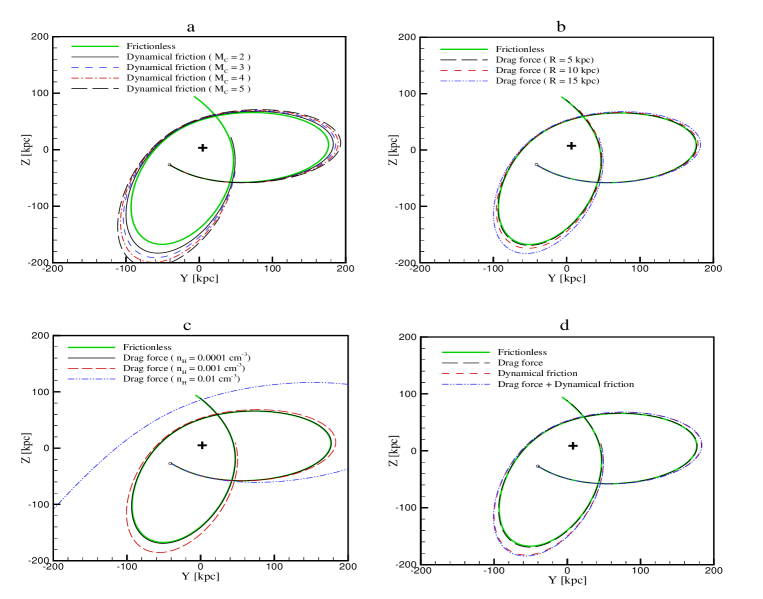
Figure 1: The effect of friction forces on the orbit of MCs. (a) The effect of dynamical friction for different value of MCs’s mass. (b) The effect of hydrodynamical drag force on the orbit of MCs for different value of MCs’s size. (c) The effect of hydrodynamical drag force on the orbit of MCs for different value of halo density. (d) Comparison of orbits for different types of friction forces with that of frictionless orbit. Here is shown that the effect of dynamical friction is more significant than the hydrodynamical drag force. The duration of evolution is $5Gyr$. The mass of MCs is in terms of $10^{10}M_{\odot}$. The initial condition selected as HR94. The plus sign denotes the Galactic position at (0,0,0). The black spot denotes the present position of MCs.

work	3D $v(x,y,z)$	$|v|$	$v_{tan}$	$v_{rad}$	$r(x,y,z)$
$GN96$	(-5,-226,194)	297	287	82	(-1.0,-40.8,-26.8)
$HR94$	(-10.06,-287.09,229.73)	367.83	351.81	107.37	(-0.85,-40.85,-27.95)
$K2$	(-91,-250,220)	345	333	92	(-0.8,-41.5,-26.9)
$K1Mean$	$(-86^{+12}_{-12},-268^{+11}_{-11},252^{+16}_{-16})$	$378^{+18}_{-18}$	$367^{+18}_{-18}$	$89^{+4}_{-4}$	(-0.8,-41.5,-26.9)
$M05$	(-4.3,-182.45,169.8)	249.3	237.9	74.4	(0,-43.9,-25.04)
$vdM02$	$(-56^{+36}_{-36},-219^{+23}_{-23},186^{+35}_{-35})$	$293^{+39}_{-39}$	$281^{+41}_{-41}$	$84^{+7}_{-7}$	(-0.8,-41.5,-26.9)

Table 1: Orbital parameters of LMC used in this work. The position is in $kpc$ and velocities are in $kms^{-1}$ and is measured in Galactocentric coordinate. References: Gardiner & Noguchi (1996, GN96), Heller & Rohlfs (1994, HR94), Kallivayalil et al. (2006a,b, K1 and K2), Mastropietro et al. (2005, M05), and van der Marel et al. (2002, vdM02).

(b)Hydrodynamical drag force: The hydrodynamical friction force results from the direct collision of the halo gas with the MCs while passing through the halo. The presence of hot diffused gas in the Galactic halo in hydrodynamical equilibrium with the dark halo has been proposed by White and Frenk (1991). To explain some ionization features discovered in MS, the baryonic halo gas should have a temperature in order of $\sim 10^{6}K$ distributed at a radius larger than $70kpc$ Sembach et al (2003); Putman et al. (2003). Constraints from the dynamics and the thermal observations propose the density of gas to be in the range of $10^{-5}$ to $10^{-4}cm^{-3}$. Assuming MCs as a dense sphere moving through the halo, the drag force on this sphere is given by:

$$F_{drag}=\frac{1}{2}C_{d}(R_{e})\rho_{g}v_{c}^{2}\pi D^{2},$$ (6)

where $C_{d}(R_{e})$ is the coefficient of drag force which is a function of Reynolds number $R_{e}$, $\rho_{g}$, the density of halo, $v_{c}$, the relative speed with respect to the gas, and $D$, the size of the Clouds. The time scale of the hydrodynamical friction force can be given by $T_{drag}\sim M_{MCs}v_{c}/F_{drag}$. which implies $T_{drag}/T_{dyn}\sim M_{MCs}/\rho_{g}rD^{2}$. Substituting the parameters as $r\sim 50kpc$, $D\sim 5kpc$, number density of halo $\sim 10^{-4.5}atom/cm^{3}$ and $M_{MCs}\sim 10^{10}M_{\odot}$, we obtain $T_{drag}\gg T_{dyn}$. Figures (1b) and  (1c) show the effect of friction forces appeared in equation (4) on the orbital motion of MCs. Due to the dynamical friction, MCs lose a few percent of total energy in each passage. The effect of the gaseous halo density and size of clouds on the magnitude of drag force is indicated in Figure (1). The apogalactic distance of clouds decreases gradually during the evolutionary period. Finally, we calculate the dynamics of MCs including all forces, represented in Figure (1d). Amongst the dissipative forces, the dynamical friction force is the dominant term and can deviate the orbit of MCs from that of frictionless one.

3.2 Modeling of the Magellanic Stream

In order to determine the evolution and the formation history of MS, it is essential to know the spatial location and velocities of MCs at the present time as the initial condition. As we mentioned before this initial condition suffers from the uncertainties mainly from the tangent velocity field of this structure. Different initial conditions show significantly different orbits and location of the interaction between LMC and SMC. In this regards, recently an extended analysis of the parameter space for the interaction of the Magellanic system with the MW has been done by Ruzicka et al (2007), using the genetic search algorithm combined with an approximate restricted N-body simulation (instead of fully self-consistent simulation). Also in another orbital analyzing, different sets of initial conditions have been applied to determine the first passage of LMC around the MW Besla et al. (2007). One of the main aims of this work is seeking the results that are common for different selection of initial conditions.

We use the six different sets of initial conditions listed in Table (1) and for each set, we find out the best space parameters of MW halo. Since the obtained parameters depends on the formation mechanism of the MS, we compare our results with the other studies which used other formation mechanism. For modeling the MS, we follow the continues ram pressure stripping mechanism introduced by Sofue (1994) including the dynamical and hydrodynamical friction forces. In that work it is assumed that if LMC and SMC approach to each other, this sever encounter will most likely disrupt the two galaxies to form the Magellanic bridge (a stream of HI gas between the LMC and SMC). The Magellanic bridge within SMC and LMC then has been stripped off by the ram-pressure when the MCs was moving through a hot MW halo. According to the observations, at the present time, the gaseous stuff is leaving the Magellanic bridge Brüns et al. (2005). We assume that the gas is initially distributed inside the MCs. The relative motion of MCs inside the Galactic halo makes a drag force on the gas of Magellanic bridge and due to the larger cross section of gas compare to the stars, the gas exit from the MCs. The released gas slows down by the friction force and accrete into the galactic disk and makes the MS. The equation of motion of MS particles can be written as

$$\frac{d^{2}\mathbf{r}_{MS}}{dt^{2}}=\frac{\partial}{\partial\mathbf{r}_{L}}[\phi_{MCs}(|\mathbf{r}_{MS}-\mathbf{r}_{MCs}|)+\phi_{G}(|\mathbf{r}_{MS}|)]+\mathbf{f}+F_{drag},$$ (7)

where $r_{MS}$ and $r_{MCs}$ are the distance of MS and MCs from the center of Galaxy, $\mathbf{f}$ is the dynamical friction force and $F_{drag}$ is the hydrodynamical drag force. As a simple model, MS is considered as a series of spherical clumps with the size of about $0.5kpc$ and the mass of $m=3\times 10^{6}M_{\odot}$ Sofue (1994). The first part of the MS (i.e. end of tail) is generated at the time of LMC-SMC close approach about $0.5Gyr$ ago and subsequent clumps is released from the MCs after this time. Since the dynamical friction force is proportional to the mass of the object, for these clumps, we can ignore this term in comparison with the drag force. Base on such simple model, we were able to produce a large number of trailing tail across the entire range of halo parameters values. By comparing the created MS profile with the observed data we find out the best set of halo parameters. In the next section we calculate the orbit of MS for two main category of the power-law and logarithmic models.

4 Results and discussion

In this section we calculate the equations of motion of MCs using the gravitational potential of disk, bulge and dark halo. We extract the dynamics of MS and obtain the trajectory of MS in various Galactic models. Then we reproduce the radial velocity distribution of HI in MS for different initial conditions of MCs (reported in Table 1) to compare with the observed data. For each initial condition, the best fit orbital parameters have been reported in Table (2). We assumed that the LMC and SMC form a binary system that has been in a slowly decaying orbit about the MW for roughly a Hubble time. One of the crucial points in studying the dynamics of MS is the location of the close approach and the corresponding time which depends on the velocities and positions of MCs at the present time. For the heavy halos, the collision happens at the closer distance to the present position of MCs than the light mass halos.

In what follows we use generic power-law and logarithmic halo models and extract the best values for the parameters of the model through the maximum likelihood analysis. We use $\chi^{2}$ fit to compare the deviation of the observed radial velocity from the theoretical predictions.

4.1 Logarithmic model

work	$V_{C}(km/s)$	$q$	$T_{col}[Gyr]$	$d_{min}[kpc]$	$\chi^{2}$
$GN96$	$180^{+1}_{-1}$	$0.95^{+0.05}_{-0.02}$	0.33	5.9	7.9
$HR94$	$195^{+1}_{-1}$	$0.55^{+0.07}_{-0.05}$	0.97	6.7	9.8
$K2$	$190^{+3}_{-7}$	$0.85^{+0.15}_{-0.10}$	0.25	8.2	10.5
$K1Mean$	$195^{+4}_{-5}$	$1.00^{+0.15}_{-0.07}$	0.22	7.4	8.9
$M05$	$165^{+2}_{-1}$	$1.05^{+0.07}_{-0.02}$	0.46	4.0	8.6
$vdM02$	$200^{+1}_{-4}$	$0.9^{+0.10}_{-0.02}$	0.30	10.03	8.4

Table 2: The best Parameters of logarithmic model for various initial conditions. The first column represents the corresponding reference for the initial condition of MCs. The parameters in the second and third columns ($V_{c}$ and $q$ ) have been introduced in the text. The fourth column, $T_{col}$ is the last close approach of LMC and SCM, the fifth column $d_{min}$ indicates the distance between LMC and SMC at last close approach. The last column shows the minimum $\chi^{2}$ corresponds to each initial condition. The mean value of $V_{c}$ and $q$ from the various initial conditions for MCs is $\bar{q}\sim 0.9$ and $\bar{V_{c}}\sim 187$.

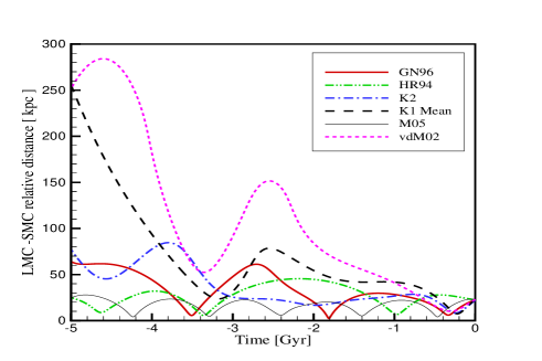
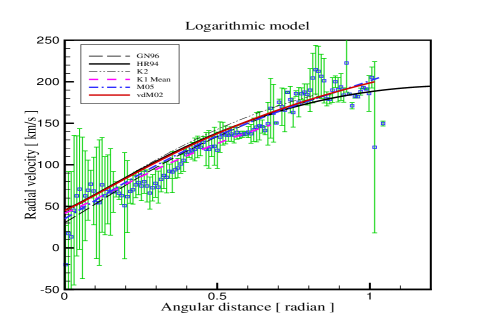
Figure 2: Relative distance of LMS and SMC as a function of time (top) and radial velocity versus angular distance along the $MS$ (bottom) for the best-fit logarithmic halo potential. Open squares show the observed radial velocity and curves correspond to that of best fit with various initial conditions.

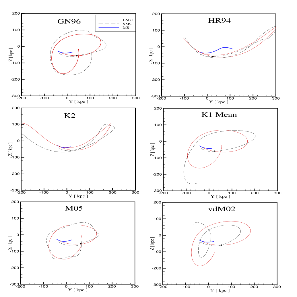
Figure 3: $Y-Z$ plane orbital path of LMC (red solid line), SMC (dashed line) and MS (blue solid line) for the best-fit logarithmic halo potential with various initial conditions. The orbital path of the LMC is not significantly affected by the SMC, however SMC’s path is deviated by LMC. MW is located at $(0,0)$. The black circle denotes the position of last close approach of LMC and SMC. The duration of orbital evolution is $5Gyr$.

We use radial velocity of MS to compare the theoretical model with the observed data. The radial velocity of MS is calculated by averaging over the data at each point of MS along the line of sight. The corresponding error bar results from the velocity dispersion of the structure which results from the stochastic motions of gas. Figures (2) represents the relative distance of LMC and SMC for six different initial conditions and the radial velocity of MS as a function of angular location for the best free parameters of the model. It should be noted that radial velocity is measured with respect to an observer located at the center of Galaxy. The zero angular distance corresponds to the position of $MSI$ (the nearest part of MS to MCs).

For each set of halo parameters, the radial velocity profile of HI clumps in MS is numerically calculated and compared with the observed radial velocity profile. The analysis repeated for various initial conditions of the clouds. The best value of model parameters ($q$ and $V_{c}$) for various initial conditions are given in Table 2. Except HR94 which prefers more oblate halo, for the other sets of initial conditions, better agreement between the model and observational data is achieved for nearly oblate or spherical halo. The mean value of the best fit parameters, averaging over the different sets of initial conditions are $\bar{q}\sim 0.9$ with $\bar{V_{c}}\sim 187kms^{-1}$. These values are in agreement with the flattening of the MW halo potential obtained by Helmi (2004) and are also compatible with the implied value of circular velocity of MW Mcgaugh (2008); Xue et al. 2008 .

Finally we present the projected trajectory of LMC, SMC and MS in Figure (3) for various initial conditions. The MCs move on rosset-shape orbits except the case of HR94 and K2 which have the banana-shape trajectory. The apogalactic distance of LMC decreases gradually during the evolutionary period, which reflects the effect of dynamical friction. According to Figure (3), for two initial conditions represented by K2 and K1-mean, the spatial extension of MS is shorter than the observed size, while for the case of HR94 it is longer than the observed size. This result arises from the longer time for the last close approach ($T_{col}$) in HR94. The minimum relative distance of the LMC and SMC at the last close approach ($d_{min}$) and the corresponding time is calculated and presented in Table 2.

4.2 Power-law model

Following the logarithmic model we calculate the radial velocity distribution of MS in the power-law galactic model and compare it with the observed data. In the power-law model we have $4$ free parameters: the asymptotic velocity, $V_{a}$, the halo flattening, $q$, the core radius, $R_{c}$ and the rising or falling parameter of rotation curve $\beta$. The best value of parameters for each initial conditions are given in Table 3. The mean value of the best fit parameters averaging over the different set of initial conditions are $\bar{q}\sim 0.85$, $\bar{V_{a}}\sim 168$, $\bar{R_{c}}\sim 17$, and $\bar{\beta}\sim-1.7$. Again similar to the logarithmic halo model, a better agreement with observational data is generally achieved for nearly oblate or spherical ($q\leq 1$) halo model.

work	$V_{a}[km/s]$	$R_{c}[kpc]$	$\beta$	$q$	$T[Gyr]$	$d[kpc]$	$\chi^{2}$
$GN96$	$185^{+2}_{-2}$	$17^{+2}_{-4}$	$0.10^{+0.06}_{-0.20}$	$0.95^{+0.05}_{-0.03}$	0.33	5.9	7.86
$HR94$	$165^{+4}_{-5}$	$13^{+6}_{-4}$	$-0.20^{+0.14}_{-0.04}$	$0.60^{+0.12}_{-0.04}$	0.76	4.8	9.5
$K2$	$160^{+5}_{-6}$	$13^{+4}_{-2}$	$-0.20^{+0.02}_{-0.09}$	$0.80^{+0.18}_{-0.08}$	0.23	7.5	8.7
$K1Mean$	$165^{+7}_{-10}$	$17^{+6}_{-7}$	$-0.20^{+0.10}_{-0.10}$	$0.75^{+0.17}_{-0.10}$	0.22	6.5	8.5
$M05$	$145^{+10}_{-2}$	$21^{+3}_{-4}$	$-0.30^{+0.06}_{-0.10}$	$1.00^{+0.04}_{-0.03}$	0.41	2.1	7.2
$vdM02$	$190^{+2}_{-2}$	$21^{+3}_{-3}$	$-0.20^{+0.04}_{-0.04}$	$1.00^{+0.03}_{-0.06}$	0.28	9.45	7.5

Table 3: The best parameters of power-law model for each sets of initial condition. The parameters of this model is introduced in equation (2). The mean value of the best fit parameters averaging over the different set of initial conditions are $\bar{q}\sim 0.85$ and $\bar{V_{a}}\sim 168$, $\bar{R_{c}}\sim 17$, $\bar{\beta}\sim-1.7$.

Figure (4) shows the time variation of the relative distance of LMC and SMC for the last 5 Gyr and radial velocity in Galactic frame as a function of angular separation of MS with respect to MSI. Different curves corresponds to various initial conditions of the MCs. The projected trajectory of LMC, SMC and MS for the best values of the parameters of model is shown in Figure (5). Similar to the logarithmic model, in the case of HR94, the generated MS extends longer than the observation. From the equations of motion, the minimum relative distance of the LMC and SMC at the last close approach and the corresponding time is also calculated (see Table 3).

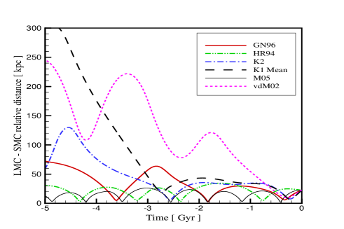
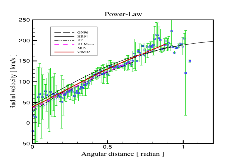
Figure 4: Relative distance of LMS and SMC as a function of time (top) and radial velocity versus angular distance along the $MS$ (bottom) for the best-fit Power-law halo potential. Open squares show the observed radial velocity and curves correspond to that from the best fit with various initial conditions.

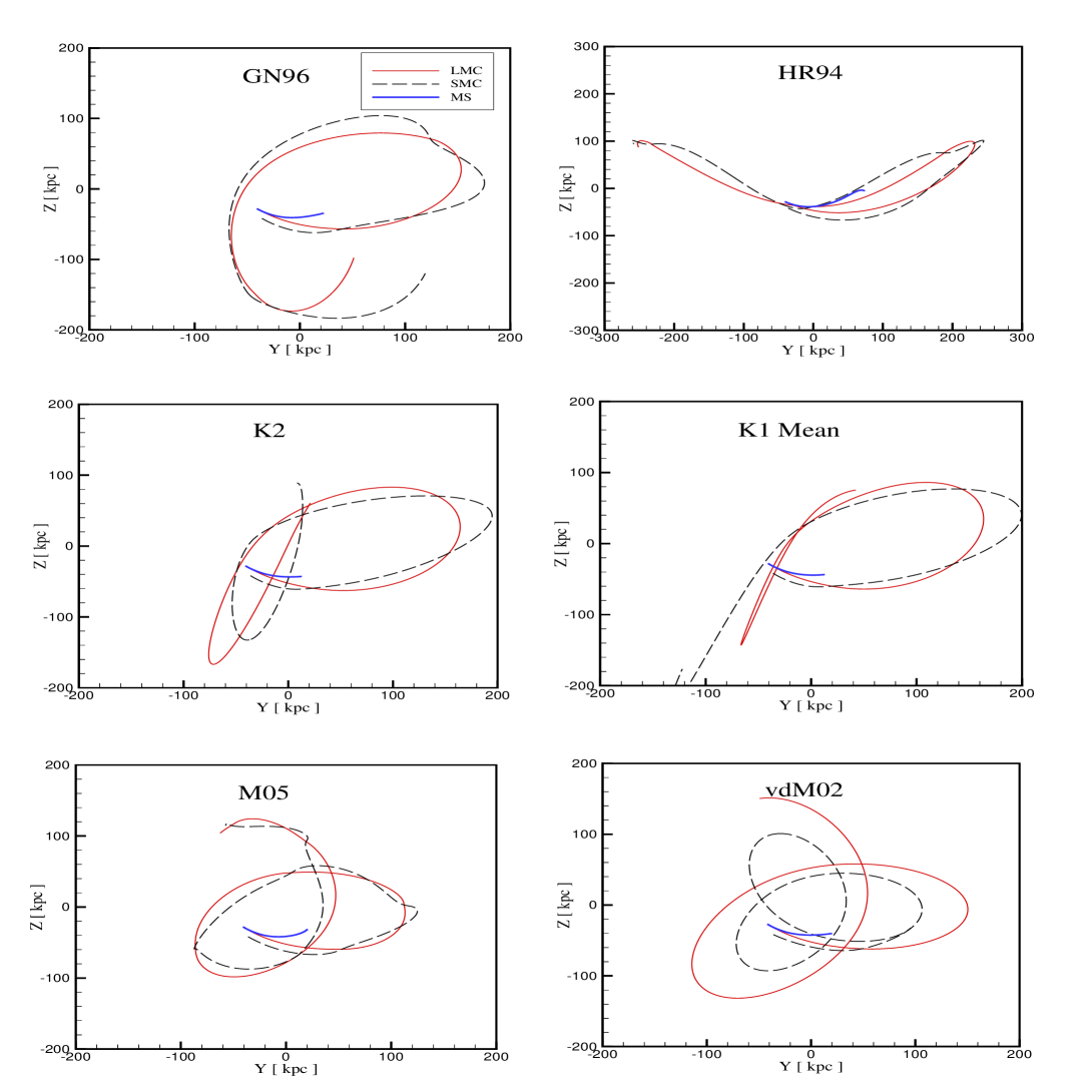
Figure 5: The $Y-Z$ plane orbital path of LMC (red solid line), SMC (dashed line) and MS (blue solid line) for the best-fit power-law halo potential with various initial conditions. The orbital path of the LMC is not significantly affected by the SMC, however SMC’s path is deviated by LMC. MW is located at $(0,0)$. The black circle denotes the position of last close approach of LMC and SMC. The duration of orbital evolution is $5Gyr$.

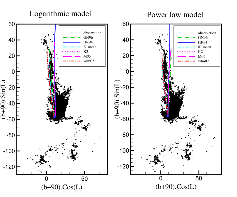
Figure 6: HI distribution of MS from the data Brüns et al. (2005) is plotted as a polar projection for both logarithmic and power law model. The axis are the galactic longitude and latitude as defined in the axis label. The blue dot indicates the location of the LMC. The colored lines are the projection of spatial distribution of the MS which theoretically determined by several initial conditions under logarithmic and power-law MW model. Note that the different initial conditions almost does match the data. The HR94 result is indistinguishable from that of the M05 result and both deviate from the location of the tip of MS. The similar situation occur for the vdm02, K1mean and K2 velocities.

In order to visualize the compatibility of simulated MS with the observational distribution of the stream, we plot the projected spatial distribution of MS corresponding to the different initial conditions in Figure (6). We find little deviation in the projected distribution of MS with the theoretical predictions. However, there is a significant difference between the observation and the theoretical prediction in the case of HR94 and M05 for both halo models. Although the GN96 initial condition could fit with the MS in logarithmic model, it no longer traces the MS in power-law model. Figure (6) shows that in the logarithmic model the projected MS using the GN96, vdm02, K1mean and K2 initial conditions are nearly indistinguishable and almost overlaying HI data of MS. The similar results valid for power-law model except for the case of GN96.

5 Conclusion

Summarizing this work, we studied the formation of Magellanic Stream as a consequence of interaction of the Magellanic Clouds and MW. We used a continuous ram-pressure model for simulating MS. The dynamics of MS is used to put constrain on the shape of Galactic halo. In this model the particles of halo sweep the hydrogen gas of the Magellanic Clouds while moving through the halo. At the first step we reconstruct the orbital motion of the Magellanic Clouds as a three body system of Galaxy, LMC and SMC taking into account the initial condition of last two objects at the present time. In this scenario, at the last close approach of LMC and SMC a part of their gas has been ejected from the system to form Magellanic stream. While the Magellanic Clouds gradually spiral towards the Galaxy, the stream of gas releases from this system and makes Magellanic Stream. We showed that the drag force of halo on the stream is larger compare to that on the Magellanic Clouds while the dynamical friction force on Magellanic Clouds is larger than on Magellanic Stream. These friction forces causes the orbit of these structures to spiral faster toward the Galaxy. Using this simple model for generating MS, we were able to find the best parameters of halo model, comparing the radial velocity of Stream with the theoretical model.

In order to see the effect of different shape of Galactic potentials, we took two generic logarithmic and the power-law potentials for the Galactic halo and calculate the dynamics of Magellanic Stream for these potentials. Since there is a large uncertainty in the initial conditions of MCs at the present time, we applied six different initial conditions reported in the literature Besla et al. (2007). Finally we compared the numerical results of radial velocity profile of MS with the observed data. Using the likelihood analysis we found that Galactic halo is nearly oblate almost in all the initial conditions for the two galactic halo models. Furthermore, the preferred value for the flattening parameter in our analysis is in agreement with the recent analysis which has employed a tidal model for the MS and logarithmic potential for the Galactic halo Ruzicka et al. (2007). In addition, the corresponding value for circular velocity is compatible with the recent measurement based on SDSS data Xue et al. 2008 and is in agreement with the rotation curve analysis Mcgaugh (2008).

We would like to thank C. Brüns provided us recent data of Parkes HI survey of Magellanic System and his useful comments.

References

- Besla et al. (2007) Besla, G. et al. 2007, ApJ 668, 949.
- Binney and Tremaine (1987) Binney S., Tremaine S. 1987, Galactic Dynamics, Princeton Univ. Press, Princeton, NJ.
- Bosma (1981) Bosma, A. 1981, AJ, 86, 1825.
- Brüns et al. (2005) Brüns, C., et al. 2005, A&A, 432, 45.
- Connors et al. (2006) Connors, T.W., Kawata, D., Gibson, B.k. 2006, MNRAS, 371, 108.
- Dubinski and Carlberg (1991) Dubinski, J., Carlberg, R. G. 1991, ApJ, 378, 496.
- Evans 1993 & (1994) Evans N. W. 1993, MNRAS, 260, 191; Evans N. W., 1994, MNRAS 267, 333
- Frenk et al. (1988) Frenk, C. S., et al. 1988, ApJ, 327, 507.
- Gardiner and Noguchi (1996) Gardiner, L. T., Noguchi, M. 1996, MNRAS 278, 191.
- Grillmair and Dionatos (2006) Grillmair, C. J., & Dionatos, O. 2006, ApJ 641, L37
- Heller and Rohlfs (1994) Heller P., Rohlfs K., 1994, A&A 291, 743.
- Helmi (2004) Helmi, A., 2004, MNRAS 351, 2, 643
- Ibata et al. (2001) Ibata, R., Lewis, G. F., Irwin, M., Totten, E., & Quinn, T. 2001, ApJ 551, 294.
- Kallivayalil et al. (2006) Kallivayalil, N., van der Marel, R. P., & Alcock, C. 2006b, ApJ, 652, 1213, [K2]
- Kallivayalil et al. (2006) Kallivayalil, N., van der Marel, R. P., Alcock, C., & et al., 2006a, ApJ 638, 772, [K1]
- Lin & Lynden-Bell (1982) Lin D. N. C., Lynden-Bell D. 1982, MNRAS 198, 707.
- Majewski et al. (2003) Majewski, S. R., Skrutski, M. F., Weinberg, M. D., & Ostheimer, J. C. 2003, ApJ 599, 1082.
- Mastropietro et al. (2005) Mastropietro C., Moore B., Mayer, L., Wadsley J and Stadel J. 2005, MNRAS 363, 521.
- Mathewson et al. (1987) Mathewson D. S., Wayte S. R., Ford V. L., Ruan K. 1987, Proc. Astron. Soc. Aust. 7, 19.
- Mcgaugh (2008) Mcgaugh, S. S., 2008, ApJ 683, 137.
- Moore and Davis (1994) Moore B., Davis, M., 1994, MNRAS 270, 209.
- Murai and Fujimoto (1980) Murai T., Fujimoto M., 1980, PASJ, 32, 581.
- Newberg et al. (2002) Newberg, H. J., et al. 2002, ApJ 569, 245.
- Odenkirchen et al. (2001) Odenkirchen, M., et al. 2001, ApJ 548, L165.
- Olling & Merrifield (2000) Olling, R. P., & Merrifield, M. R. 2000, MNRAS 311, 2, 361.
- Putman et al. (2003) Putman, M. E., Bland-Hawthorn, J., Veilleux, S., Gibson, B. K., Freeman, K. C., Maloney, P. R. 2003, ApJ 597, 948.
- Read and Moore (2005) Read, J. I., Moore, B., 2005, MNRAS 361, 971.
- Rubin & Burstein (1985) Rubin, V. C., & Burstein, D., 1985, ApJ, 297, 423.
- Ruzicka et al. (2007) Ruzicka, A., Palous, J., Theis, C. 2007, A&A 461, 155.
- Sembach et al (2003) Sembach, K. R. et al. 2003, ApJS 146, 165
- Sofue (1994) Sofue, Y. 1994, PASJ 46, 431.
- van der Marel et al. (2002) van der Marel, R. P., Alves, D. R., Hardy, E., & Suntzeff, N. B. 2002, AJ, 124, 2639 [vdM02].
- White and Frenk (1991) White, S. D. M., Frenk, C. S. 1991, ApJ, 379, 52.
- (34) Xue X.X. et al. ,2008, ApJ 684, 1143.