A galaxy-halo model of large-scale structure

Abstract

We present a new, galaxy-halo model of large-scale structure, in which the galaxies entering a given sample are the fundamental objects. Haloes attach to galaxies, in contrast to the standard halo model, in which galaxies attach to haloes. The galaxy-halo model pertains mainly to the relationships between the power spectra of galaxies and mass, and their cross-power spectrum. With surprisingly little input, an intuition-aiding approximation to the galaxy-matter cross-correlation coefficient $R(k)$ emerges, in terms of the halo mass dispersion. This approximation seems valid to mildly non-linear scales ($k\la 3{\ }h{\,}{\rm Mpc}^{-1}$), allowing measurement of the bias and the matter power spectrum from measurements of the galaxy and galaxy-matter power spectra (or correlation functions). This is especially relevant given the recent advances in precision in measurements of the galaxy-matter correlation function from weak gravitational lensing. The galaxy-halo model also addresses the issue of interpreting the galaxy-matter correlation function as an average halo density profile, and provides a simple description of galaxy bias as a function of scale.

1 Introduction

The halo model of large-scale structure has been quite successful in interpreting observations of galaxy and mass clustering. In the halo model, the dark matter in the Universe consists entirely of virialized clumps called haloes. The assumption is made that galaxies can only form within these haloes, with the number of galaxies per halo depending (primarily) on the mass of the halo, according to a halo occupation distribution (HOD).

Some of the inputs to the halo model arise from pure theory, such as the linear power spectrum. Others come from theory with some calibration with simulations, such as the mass spectrum and bias of the haloes. Yet others are entirely empirical, such as the HOD, and halo density profiles. In fact, although ideas related to the halo model have existed for decades (Neyman & Scott, 1952; Scherrer & Bertschinger, 1991), it was not until a universal halo density profile was discovered from simulations (Navarro, Frenk & White, 1997) that the halo model began to really develop (Peacock & Smith, 2000; Seljak, 2000; Ma & Fry, 2000; Scoccimarro et al., 2001; Berlind & Weinberg, 2002). For a review, see Cooray & Sheth (2002). There are some things about the halo model which unsettle us somewhat; for instance, the cosmic web seen in observations and numerical simulations is not directly explained in the halo model as it currently stands. However, the halo model has matured to the degree that it seems to be able to help constrain cosmological parameters (Seljak et al., 2005a, b). As observations and simulations improve, it is likely that the halo model will evolve to match observables from them arbitrarily well as theoretical ingredients are added to it, without fundamental conceptual changes.

In this paper, we approach the problem of interpreting large-scale structure observations with a different philosophy, investigating how much can be learned with the observations themselves, with as little theoretical input as possible. The galaxy power spectrum $P_{gg}$ is taken as the fundamental quantity, even though it is not known how to produce it theoretically at present. Haloes (or subhaloes; they are not differentiated in the model) are attached to galaxies, not the other way around. The galaxy-matter power spectrum $P_{gm}$ and the matter power spectrum $P_{mm}$ (or, more accurately, their two-halo terms) are then simple convolutions of $P_{gg}$ with average halo density profiles. Some added information about large-scale bias and the halo mass dispersion yields a surprising amount of information about the galaxy-matter cross-correlation coefficient, the bias, and the cross-bias.

We emphasize that this galaxy-halo model is not meant to be a competitor to the standard halo model, which could be called the ‘largest virialized’ halo model, since each halo in the standard halo model is the largest possible virialized structure. The galaxy-halo model as presented in this paper is not a formalism which may be used to compare to all conceivable observations, although it may evolve to be more encompassing in the future. It is currently restricted because it has few ingredients, and it is not known how to obtain the main ingredient $P_{gg}$ a priori. In fact, we are surprised that because it is simpler, the galaxy-halo model was not developed before the halo model. The above criticism of the halo model (that it does not produce the cosmic web) applies to the galaxy-halo model, too. However, the simplicity of the galaxy-halo model has benefits; it allows for some intuitive insights, and for interpretation of some observations with few assumptions.

2 Ratios of clustering statistics

It can be useful to form ratios of two-point statistics (the power spectrum and the correlation function; see e.g. Peebles, 1980; Hamilton, 2005) which measure the clustering of matter and galaxies. In Fourier space, the (squared) bias is $b^{2}(k)\equiv P_{gg}(k)/P_{mm}(k)$, the ratio of the galaxy power spectrum to the matter power spectrum. The (squared) galaxy-matter cross-correlation coefficient is $R^{2}(k)\equiv P_{gm}(k)^{2}/[P_{gg}(k)P_{mm}(k)]$, where $P_{gm}$ is the galaxy-matter cross power spectrum. With the advent of galaxy-matter observations from weak lensing, the ‘cross-bias’ has also been used: $b/R\equiv P_{gg}(k)/P_{gm}(k)$.

The same ratios may also be defined in real space, using correlation functions instead of power spectra; recent observations (e.g. Sheldon et al., 2004) have tended to favor the real-space description. There are at least two good reasons for this: $\xi_{gm}$, and not $P_{gm}$, is more directly measured from weak-lensing observations; and also, $\xi$ is easier to understand intuitively and visually.

However, the theoretically preferred representation is in Fourier space, for several reasons. Most relevantly for the present paper, the Schwarz inequality imposes a mathematical constraint on the cross-correlation coefficient $R(k)$ when expressed in Fourier space. The Schwarz inequality requires that $\langle|\delta_{m}({\bf k})\delta_{g}(-{\bf k})|\rangle^{2}\leq\langle|\delta_{g}({\bf k})|^{2}\rangle\langle|\delta_{m}({\bf k})|^{2}\rangle$. If and only if the galaxy and matter power spectra include the shot noise, this gives

$$R^{2}(k)=\frac{P_{gm}(k)^{2}}{P_{gg}(k)P_{mm}(k)}\leq 1.$$ (1)

The shot noise in $P_{mm}$ is negligible because dark-matter particles are practically infinitesimal on all astrophysically relevant scales. However, the shot noise in $P_{gg}$ may be comparable to the galaxy clustering signal, and so including or excluding the shot noise in $P_{gg}$ makes a significant difference.

The galaxy-matter cross-correlation coefficient $R$ has been discussed (Dekel & Lahav, 1999; Pen, 1998; Tegmark & Bromley, 1999; Taruya & Soda, 1999; Seljak & Warren, 2004) as a measure of the stochasticity, or scatter, in the relationship between the galaxy overdensity $\delta_{g}$ and the matter overdensity $\delta_{m}$. This interpretation of $R$ is clearest when the Fourier-space representation of $R$ is used, and when the shot noise is included in $P_{gg}$; thus, we advocate defining $R$ in this manner. Then $R(k)$ has a straightforward physical meaning: it is unity on large scales where $\delta_{g}(k)$ and $\delta_{m}(k)$ are simply related, and decreases on small, nonlinear scales where significant scatter exists in the relationship.

3 The standard halo model

Now we will outline the standard halo model, drawing primarily on Cooray & Sheth (2002) and Seljak (2000). For the matter power spectrum $P_{mm}(k)$, the following ingredients are necessary: the linear power spectrum $P_{\rm lin}(k)$, the number density of haloes as a function of mass $n(M)dM$, the large-scale bias as a function of halo mass, $b(M)$, and the average Fourier-transformed density profile of a halo of mass $M$, $y(k,M)$. This density profile is normalized to be unity at $k=0$:

$$y({\bf k},M)=\frac{1}{M}\int\rho({\bf r},M)\exp(-i{\bf k}\cdot{\bf r})d^{3}r,$$ (2)

where $\rho({\bf r},M)$ is the average real-space density profile of a halo of mass $M$. For a spherically-symmetric density profile $\rho(r,M)$, this becomes

$$y(k,M)=\frac{4\pi}{M}\int_{0}^{\infty}\frac{\sin kr}{kr}\rho(r,M)r^{2}dr.$$ (3)

The power spectrum is a sum of one-halo ($1h$) and two-halo ($2h$) terms:

$$P_{mm}(k)=P_{mm}^{1h}(k)+P_{mm}^{2h}(k),$$ (4)

where

$$P_{mm}^{1h}(k)=\int y(k,M)^{2}\frac{n(M)M^{2}}{{\rho}^{2}}dM,$$ (5)

and

$$P_{mm}^{2h}(k)=P_{\rm lin}(k)\left[\int b(M)y(k,M)\frac{n(M)M}{\rho}dM\right]^{2}.$$ (6)

Here, $\rho$ is the average matter density.

With galaxies come a few more ingredients: a halo occupation distribution $(N_{\rm gal}|M)$ giving the distribution of the number of galaxies inside a halo of mass $M$, giving a total galaxy number density $n_{\rm gal}$, and a quantity $y_{\rm gal}(k)$, which describes the average galaxy density profile of a halo, in general different from its matter density profile. The galaxy-matter power spectrum $P_{gm}$ and the galaxy power spectrum $P_{gg}$ are also sums of $1h$ and $2h$ terms:

$$P_{gm}^{1h}(k) = \int y(k,M)y_{\rm gal}(k,M)^{p-1}$$ (7)

$$\times\frac{\langle N_{\rm gal}|M\rangle}{n_{\rm gal}}\frac{n(M)M}{\rho}dM;$$

$$P_{gm}^{2h}(k) = P_{\rm lin}(k)\int y_{\rm gal}(k,M)\frac{\langle N_{\rm gal}|M\rangle}{n_{\rm gal}}b(M)n(M)dM$$ (8)

$$\times\int y(k,M)b(M)\frac{n(M)M}{\rho}dM;$$

$$P_{gg}^{1h}(k) = \int y(k,M)y_{\rm gal}(k,M)^{p}$$ (9)

$$\times\frac{\langle N_{\rm gal}(N_{\rm gal}-1)|M\rangle}{n_{\rm gal}^{2}}n(M)MdM;$$

$$P_{gg}^{2h}(k) = P_{\rm lin}(k)$$ (10)

$$\times\left[\int y_{\rm gal}(k,M)\frac{\langle N_{\rm gal}|M\rangle}{n_{\rm gal}}b(M)n(M)dM\right]^{2}.$$

Here, $p$ is 2 if there is more than one galaxy per halo, and 1 otherwise; this arises from an assumption that there is a galaxy at the centre of each halo of sufficient mass. (See Cooray & Sheth 2002 for more explanation.)

4 The galaxy-halo model

A ‘galaxy halo’ is defined in this paper to be a dark-matter halo around a galaxy. As in the standard halo model, all power spectra in the galaxy-halo model are sums of one-halo ($1h$) and two-halo ($2h$) terms. These could be called one-galaxy and two-galaxy terms, since the fundamental objects in the galaxy-halo model are galaxies. However, galaxies in the galaxy-halo model are pointlike objects. It is in their haloes that matter is found, and where the galaxy-matter and matter power spectra measure the clustering.

Even though the $1h$ and $2h$ terms in the galaxy-halo model share labels with their counterparts in the standard halo model, the terms in the two models differ conceptually, and generally differ numerically as well. That is, the $1h$ and $2h$ terms get different shares of the total power spectra in the galaxy-halo model than in the standard halo model.

Since the galaxy power spectrum $P_{gg}$ is one of the inputs of the galaxy-halo model, the expressions for it are extremely simple. The two-halo term $P_{gg}^{2h}$ is just the galaxy power spectrum without shot noise. To emphasize that it is a fundamental input into the model, we simply denote $P_{gg}^{2h}$ as $P$. There is also a one-halo term in the full $P_{gg}$, which is the shot noise $1/n$, where $n$ is the total number density of galaxies. So, the two terms in $P_{gg}$, with the shot noise included, are

$$P_{gg}(k)=P_{gg}^{2h}(k)+P_{gg}^{1h}(k)=P(k)+1/n.$$ (11)

Dark-matter halo density profiles affect the other power spectra, $P_{gm}$ and $P_{mm}$. First we discuss what they are in a simple, single-mass model, and then in a more realistic model with a distribution of halo masses.

4.1 Single-mass model

In this section appears a highly simplified model, some of the results of which carry over to the next, more realistic model. Consider a population of galaxies of number density $n$ and power spectrum $P(k)$, and with haloes of identical masses and identical, spherically symmetric density profiles. The density profile $\rho(r)$ Fourier-transforms into $y(k)$, in the same manner as in eq. (3). The density profile must be well-behaved in the sense that as $r\to\infty$, $\rho(r)\to 0$ in such a way that $y(k)\to 1$.

Both the $1h$ and $2h$ terms of the galaxy-matter power spectrum depend on the Fourier-transformed density profile $y(k)$. The pairs comprising the $1h$ term are galaxies with dark-matter particles in their own haloes:

$$P_{gm}^{1h}(k)=n^{-1}y(k).$$ (12)

The $2h$ term is the power spectrum of galaxies with dark-matter particles in other haloes; it is a product in Fourier space of the galaxy power spectrum $P(k)$ with the average halo profile $y(k)$.

$$P_{gm}^{2h}(k)=P(k)y(k).$$ (13)

The matter power spectrum is similarly defined:

$$P_{mm}^{1h}(k)=n^{-1}y(k)^{2},$$ (14)

$$P_{mm}^{2h}(k)=P(k)y(k)^{2}.$$ (15)

This simple model yields simple formulae for the bias $b(k)$ and the cross-correlation coefficient $R(k)$. The (squared) bias, excluding the shot noise from $P_{gg}$, is

$$b^{2}_{\rm-sn}(k)=\frac{P(k)}{P_{mm}^{2h}(k)+P_{mm}^{1h}(k)}=\frac{P(k)}{P(k)+n^{-1}}y(k)^{-2}.$$ (16)

If the galaxy power spectrum includes the shot noise, the bias is simply

$$b^{2}(k)=y(k)^{-2}.$$ (17)

The equation for $R^{2}(k)$ (where $P_{gg}$ includes the shot noise) is even simpler:

$$R^{2}(k)=\frac{[P_{gm}^{2h}(k)+P_{gm}^{1h}(k)]^{2}}{[P(k)+n^{-1}][P_{mm}^{2h}(k)+P_{gm}^{1h}(k)]}=1.$$ (18)

This makes sense: galaxies and matter are perfectly cross-correlated if all galaxy haloes are identical.

4.2 Multiple-mass model

Now, more realistically, suppose that there is a distribution of halo masses and shapes (which need not be spherically symmetric). As a pedagogical aid to those familiar with the halo model, we will point out how various terms change or disappear using the galaxy-halo model. In doing this, we do not mean to imply that the galaxy-halo model is a subset of the halo model, in which additional assumptions are made. The fundamental assumptions of the two models differ.

In the halo model, galaxies are put into haloes, while in the galaxy-halo model, haloes are put around galaxies. So, in the galaxy-halo model, the HOD (which does not explicitly appear) is identically 1, and $y_{\rm gal}$ is unnecessary. The galaxy power spectrum $P$ is the fundamental quantity, so $P_{\rm lin}$ does not appear. The bias as a function of $M$, $b(M)$, also is not needed, since it is subsumed into $P$. However, there is still a large-scale bias $b_{0}$ multiplying the three $2h$ terms; as $k\to 0$, $P_{gg}^{2h}(k)=b_{0}P_{gm}^{2h}(k)=b_{0}^{2}P_{mm}^{2h}(k)$.

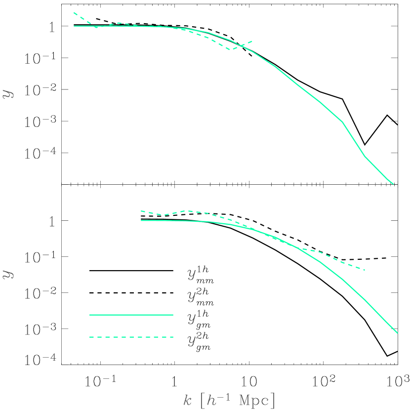
Figure 1: For two different halo populations, comparisons of the average Fourier-transformed density profiles $y_{gm}^{1h}$, $y_{gm}^{2h}$, $y_{mm}^{1h}$, and $y_{mm}^{2h}$, as measured from $N$-body simulations described by Neyrinck, Hamilton & Gnedin (2004). The mass threshold defining the top panel’s halo sample is $3\times 10^{13}{\ }h^{-1}{\,}{\rm Mpc}$; the bottom panel’s threshold is smaller by a factor of 512. The $1h$ profiles $y_{gm}^{1h}$ and $y_{mm}^{1h}$ were obtained from $P_{gm}^{1h}$ and $P_{mm}^{1h}$ (measured by Fourier-transforming $\xi_{gm}^{1h}$ and $\xi_{mm}^{1h}$) using eqs. (19) and (21). The $2h$ profiles $y_{gm}^{2h}$ and $y_{mm}^{2h}$ were measured from $P_{gm}^{2h}$, $P_{mm}^{2h}$, and $P$ using eqs. (24) and (25). These latter two equations require an estimate of the large-scale bias $b_{0}$ for each halo sample. For the top panel, we fitted $b_{0}=1$ by hand, and for the bottom panel, we used the value $b_{0}=0.75$ used for Fig. 6, which is a plot of the bias from the same halo sample.

Let the total number density of galaxies be denoted $n=\int n(M)dM$, and the total mass density be denoted $\rho=\int n(M)MdM$. Here, $n(M)dM$ is the number density of galaxy haloes of a given mass; henceforth, $n$ denotes the total galaxy number density unless it explicitly appears as a function of mass. Not surprisingly, the expressions for $P_{gm}$ and $P_{mm}$ become more complicated when there is a distribution of masses. It is still straightforward, though, to express the $1h$ terms. The average Fourier-transformed density profile as a function of mass $y(k,M)$ is the average of $y(k)$ over haloes of mass $M$, and the mean-square $y^{2}(k,M)$ is the average of $y(k)^{2}$. Assuming a large enough volume that departures from isotropy vanish, these average halo profiles must be spherically symmetric, and thus have zero imaginary components. The density profiles comprising $P_{gm}^{1h}$ are averaged weighting by the product of the number density of galaxies and the mass density:

$$P_{gm}^{1h}(k)=\frac{1}{n\rho}\int{y(k,M)n(M)MdM}=n^{-1}y_{gm}^{1h}(k),$$ (19)

where $y_{gm}^{1h}$ is a mass-weighted average halo profile

$$y_{gm}^{1h}(k)\equiv\frac{\int{y(k,M)n(M)MdM}}{\int{n(M)MdM}}.$$ (20)

The density profiles comprising $P_{mm}^{1h}$ are averaged weighting by the mass squared:

$$P_{mm}^{1h}(k)=\frac{1}{\rho^{2}}\int{y^{2}(k,M)n(M)M^{2}dM}=\frac{\mu}{n}y_{mm}^{1h}(k)^{2},$$ (21)

where

$$y_{mm}^{1h}\equiv\sqrt{\frac{\int{y^{2}(k,M)n(M)M^{2}dM}}{\int{n(M)M^{2}dM}}},$$ (22)

and $\mu$ is a dimensionless mean-square halo mass,

$$\mu\equiv\langle M^{2}\rangle/\langle M\rangle^{2}\geq 1.$$ (23)

Not as much can be said about the $2h$ terms with the assumptions made so far, primarily because the large-scale bias factor of a set of haloes varies with their mass. This behaviour can be modeled (e.g. Mo & White, 1996), but to our knowledge, such a model has not been formulated which counts subhaloes as haloes, as in the galaxy-halo model. Even if there were such a model, adding it to the galaxy-halo model would cause a significant increase in the galaxy-halo model’s complexity, which we wish to avoid.

However, one thing may be safely assumed about the $2h$ terms: on large-enough scales (where the $1h$ terms are negligible, and all average Fourier-transformed density profiles are unity), the cross-correlation coefficient $R(k)=1$. To see this, suppose the universe consists of regions large enough so that the galaxy bias in each region is entirely local (Coles, 1993) and is statistically independent of the bias in other regions. In the limit $k\to 0$, a measurement of $R(k)$ requires averaging over a number of regions which goes to infinity, squeezing the variance of the biases in different regions to zero. This gives $R(k\to 0)=1$. Assuming as much, the following equations hold:

$$P_{gm}^{2h}(k) = P(k)\frac{y_{gm}^{2h}(k)}{b_{0}};$$ (24)

$$P_{mm}^{2h}(k) = P(k)\left[\frac{y_{mm}^{2h}(k)}{b_{0}}\right]^{2}.$$ (25)

Here, $b_{0}\equiv\lim_{k\to 0}\sqrt{P(k)/P^{2h}_{mm}(k)}$ is a large-scale bias (usually of order unity) and $y_{gm}^{2h}(k)$ and $y_{mm}^{2h}(k)$ are effective average halo density profiles, defined to be unity as $k\to 0$. These average halo density profiles have no imaginary component, by construction, since they are defined in eqs. (24) and (25) in terms of other real quantities.

In general, $y^{1h}$ differs from $y^{2h}$ (for both galaxy-matter and matter power spectra) because halo density profiles change systematically with the clustering strength of the haloes, and $y_{gm}$ differs from $y_{mm}$ (for both $1h$ and $2h$ terms) because the $y_{mm}$ is a root-mean-square average, whereas $y_{gm}$ is a straight average. Even though these terms typically differ, below we will explore what emerges under the approximations that $y^{1h}=y^{2h}$ and $y_{gm}=y_{mm}$.

Figure 1 compares these four average Fourier-transformed density profiles $y_{gm,mm}^{1h,2h}$, for galaxies placed at the centres of two different sets of haloes from $N$-body simulations, characterized by large (top) and small (bottom) mass thresholds. For each panel, the profiles do not correspond exactly, but they are similar. The agreement is better using a large mass threshold because excluding small haloes narrows the distributions of halo masses and density profiles.

Assuming that $y_{gm}^{1h}=y_{gm}^{2h}\equiv y_{gm}$, and $y_{mm}^{1h}=y_{mm}^{2h}\equiv y_{mm}$, the expressions for $P_{gm}$ and $P_{mm}$ simplify:

$$P_{gm}(k) \approx [P(k)/b_{0}+1/n]y_{gm}(k);$$ (26)

$$P_{mm}(k) \approx [P(k)/b_{0}^{2}+\mu/n]y_{mm}(k)^{2}.$$ (27)

With these power spectra in hand, it is possible to calculate ratios between them: the bias $b(k)$, the cross-bias $b/R=P_{gg}/P_{gm}$, and the cross-correlation coefficient $R(k)$. Here are equations for the bias (squared) $b^{2}\equiv P_{gg}/P_{mm}$, excluding the shot noise from $P_{gg}$:

$$b^{2}_{\rm-sn}(k) = \frac{P}{P(y_{mm}^{2h}/b_{0})^{2}+(\mu/n)(y_{mm}^{1h})^{2}}$$ (28)

$$\approx \frac{P}{P/b_{0}^{2}+\mu/n}{y_{mm}}^{-2}.$$ (29)

Equation (29) follows if $y_{mm}^{1h}=y_{mm}^{2h}$. If the shot noise is included in $P_{gg}$, then eq. (29) becomes

$$b^{2}(k)\approx\frac{P+n^{-1}}{P/b_{0}^{2}+\mu/n}{y_{mm}}^{-2}.$$ (30)

Equation (29) contains the general features in the bias (excluding the shot noise from $P_{gg}$) which have been observed from simulations and from the halo model (Seljak 2000). On large scales, the halo profiles in real space go to zero [and thus $y_{mm}(k)\to 1$], and the galaxy-matter two-halo term overwhelms the one-halo term [$P(k)/b_{0}^{2}\gg\mu/n$]. Thus, as expected, the only signal on large scales is the large-scale bias, and $b_{\rm-sn}(k)=b_{0}$. On intermediate scales, where the two-halo and one-halo terms in the matter power spectrum are comparable [$P(k)/b_{0}^{2}\approx\mu/n$], assuming that $y_{mm}(k)\approx 1$ still holds, the bias decreases. On small scales, the one-halo term dominates [$P(k)/b_{0}^{2}\ll\mu/n$], and so the behaviour of the bias depends on whether $P(k)$ or $y_{mm}(k)^{2}$ decreases faster as $k\to\infty$. Generally, $y_{mm}(k)^{2}$ decreases faster, forcing the bias upward. If $P_{gg}$ includes the shot noise, then the bias always increases with $k$ at small scales.

The cross-bias $b/R$, keeping the shot noise in $P_{gg}$, is

$$\frac{b}{R} \equiv \frac{P_{gg}}{P_{gm}}=\frac{P+n^{-1}}{Py_{gm}^{2h}/b_{0}+n^{-1}y_{gm}^{1h}}$$ (31)

$$\approx \frac{P+n^{-1}}{P/b_{0}+n^{-1}}{y_{gm}}^{-1}.$$ (32)

Equation (32) follows if $y_{gm}^{1h}=y_{gm}^{2h}$.

A formula with few inputs also emerges for the cross-correlation coefficient $R^{2}\equiv P_{gm}^{2}/(P_{gg}P_{mm})$. Including the shot noise in $P_{gg}$,

$$R^{2}(k) = \frac{(Py_{gm}^{2h}/b_{0}+n^{-1}y_{gm}^{1h})^{2}}{(P+n^{-1})[P(y_{mm}^{2h}/b_{0})^{2}+(\mu/n)(y_{mm}^{1h})^{2}]}$$ (33)

$$\approx \frac{(P/b_{0}+n^{-1})^{2}}{(P+n^{-1})(P/b_{0}^{2}+\mu/n)}\left(\frac{y_{gm}}{y_{mm}}\right)^{2}$$ (34)

$$\approx \frac{(P/b_{0}+n^{-1})^{2}}{(P+n^{-1})(P/b_{0}^{2}+\mu/n)}.$$ (35)

Equation (34) is true if $y_{mm}^{1h}=y_{mm}^{2h}$ (and similarly for $y_{gm}$), and for eq. (35), a more extreme assumption is made, that $y_{gm}=y_{mm}$. Since $y_{gm}$ is weighted by mass, and $y_{mm}$ by mass squared, the latter assumption will only be valid if halo profiles do not depend on mass, which is almost certainly not the case. Excluding the shot noise in $P_{gg}$ turns $(P+n^{-1})$ into $P$ in the denominator in eqs. (34) and (35).

In eq. (35), on large scales, $P$ dominates both $n^{-1}$ and $(\mu/n)$, so $R^{2}$ approaches unity. On small scales, $P$ is small, and so $R^{2}$ approaches $1/\mu$. More specifically, under these approximations, $R^{2}$ is an interpolation between 1 (its $2h$ value) and $1/\mu$ (its $1h$ value), weighted by the respective matter terms:

$$R^{2}(k) \approx \frac{\left[\left(P+\frac{1}{n}\right)\left(\frac{P}{b_{0}^{2}}+\frac{1}{n}\right)-\frac{P}{n}\left(1-\frac{1}{b_{0}}\right)^{2}\right]{y_{gm}}^{2}}{(P+n^{-1})(P_{mm}^{2h}+P_{mm}^{1h})}$$ (36)

$$\approx \frac{P_{mm}^{2h}+(1/\mu)P_{mm}^{1h}}{P_{mm}^{2h}+P_{mm}^{1h}}-\epsilon(b_{0}),$$ (37)

where we assume that $y_{gm}^{1h}=y_{mm}^{1h}$ (and similarly for the $2h$ terms). Here, $\epsilon(b_{0})$ is small if $b_{0}\approx 1$:

$$\epsilon(b_{0})=\frac{(b_{0}-1)^{2}}{1+nP+\mu b_{0}^{2}[1+1/(nP)]}.$$ (38)

Although eq. (35) is exactly true in the more general case of zero variance in halo density profile shape, it may be helpful to interpret eq. (35) by visualizing the haloes as a collection of nuggets (instead of extended haloes) of varying mass. Consider the smallest scales, $k\ga\pi/r_{\rm min}$, where $r_{\rm min}$ is the smallest intergalactic distance. Here, the Fourier-transformed galaxy and matter overdensities $\delta_{g}(k)$ and $\delta_{m}(k)$ sample at most one galaxy, and so $R^{2}(k)$ sees only the mass dispersion of galaxies. This is where the galaxy power spectrum $P\ll 1/n$, and thus $R^{2}\to 1/\mu$ in eq. (35). At progressively larger scales, $R^{2}$ samples more and more galaxies, until at the largest scales, so many galaxies enter the average that the scatter in the $\delta_{g}$-to-$\delta_{m}$ relationship vanishes, pushing $R^{2}\to 1$.

4.3 Orphans

Up to now, we have only defined a galaxy halo as a clump of dark matter (surrounding a galaxy) whose density falls off to zero at large radius. In practice, one way to define a galaxy halo sample could be to populate a set of bound dark-matter haloes and subhaloes (from a simulation, for example) with galaxies. This set of galaxy haloes could be characterized by a bound-mass or circular-velocity threshold, for example. But what about orphaned matter particles which are not bound to any galaxy halo? Such matter exists not only in voids, but in small, isolated haloes which do not meet the criteria to host a galaxy and are not bound to any larger galaxy haloes.

One way to deal with orphans is to adopt them into galaxy haloes, removing the condition that galaxy haloes must be gravitationally bound. However, it is not clear how to partition the unbound matter into galaxies, and altering the partition could significantly affect the dimensionless mean-square halo mass $\mu$.

In this paper, we exclude orphans from galaxy haloes, but they cannot be completely ignored. Even under the assumption that orphans do not affect clustering properties, excluding them in the calculation of the matter and galaxy-matter power spectra results in the wrong normalization. If $P_{gm}$ and $P_{mm}$ are calculated using only non-orphans, then the multiplicative ‘orphan factor’ $\rho_{h}/\rho$ must be applied once to $P_{gm}$ and twice to $P_{mm}$ to get the normalization right. Here, $\rho_{h}$ is the density of matter in galaxy haloes, and $\rho$ is the total matter density. ‘Orphan factors’ must be used with the bias or cross-bias, but they cancel out for the cross-correlation coefficient $R$.

Even if orphans are excluded, the question of partitioning the matter into galaxy haloes can be ambiguous. Power spectra care only about density contrasts, not about whether matter is bound to galaxies, so boundedness is not necessarily the right test to determine galaxy halo membership.

In the context of the galaxy-halo model, the best partition of matter is the one which makes the predictions of the galaxy-halo model work best. There are a few ways of judging matter partitions using this criterion. One of them is to make the approximations $y_{gm}^{1h}=y_{gm}^{2h}$ and $y_{mm}^{1h}=y_{mm}^{2h}$ hold as closely as possible, but this is hard to test over a wide range of halo samples. The easiest meaningful quantity to measure from a partition is the dimensionless mean-square mass $\mu$. Measuring $R^{2}(k)$, which is independent of the partition, and looking at its typical small-scale value, gives an idea of the ‘natural’ dimensionless mean-square halo mass. However, as displayed below in Figure 3, if haloes extend out to a scale where $P_{gg}$ is significant, $R^{2}$ may stay above its characteristic small-scale value, making $\mu$ hard to determine from $R^{2}$. There is some ambiguity in how precisely the matter should be partitioned, but that is not necessarily a bad thing, since the observed power spectra cannot depend on the partition.

5 Tests

Can the galaxy-halo model be used to extract meaningful information from observations? The galaxy-halo model contains three items which are potentially useful: simple descriptions of the galaxy-matter bias and cross-correlation coefficient; and the capacity to separate out $1h$ and $2h$ terms from an observed galaxy-matter power spectrum. This section describes tests of these items, and also explores how predictions of the galaxy-halo model vary with properties of a galaxy-halo population.

5.1 Mock halo catalogs

5.1.1 Isolating $\xi_{gm}^{1h}$

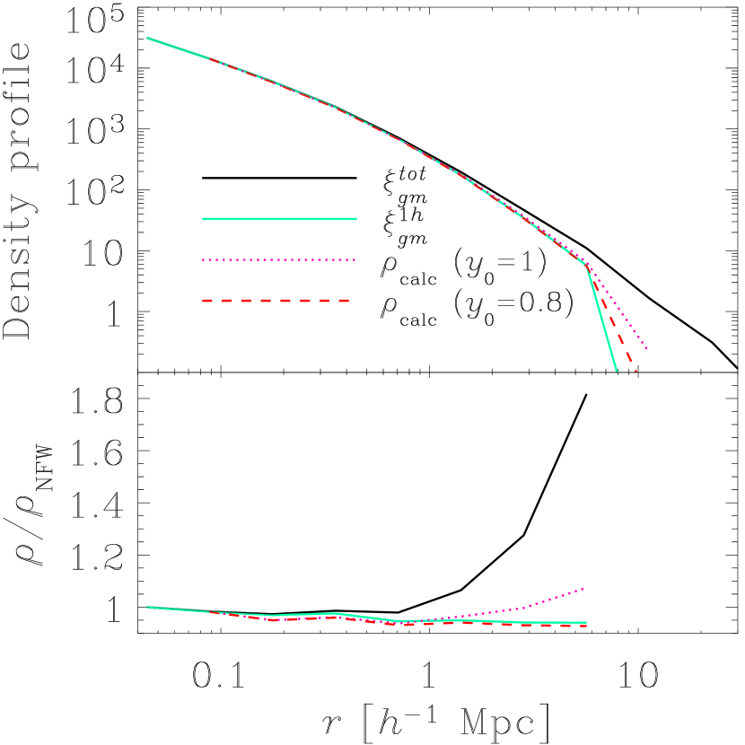
Figure 2: An NFW density profile, with a scale radius of $1{\ }h^{-1}{\,}{\rm Mpc}$ and truncated at $8{\ }h^{-1}{\,}{\rm Mpc}$, along with various attempts to recover it from a mock catalog with haloes with the profile. In the top panel, the solid black curve shows the total $1+\xi_{gm}$, and the solid grey (online, green) curve shows the one-halo $1+\xi_{gm}^{1h}$. The dashed grey (online, magenta) curve shows our attempt to isolate the $1h$ term, assuming $y=1$ in the smallest-wavenumber bin, and the dotted grey curve shows the same assuming $y=0.8$ in the smallest-wavenumber bin. The bottom panel shows the ratio of the respective curves in the top panel with the true NFW profile. The curves disappear for $r>8{\ }h^{-1}{\,}{\rm Mpc}$ (actually, $6{\ }h^{-1}{\,}{\rm Mpc}$, the centre of the bin which goes up to $8{\ }h^{-1}{\,}{\rm Mpc}$) because the input profile is truncated there.

The galaxy-matter correlation function $\xi_{gm}$ is sometimes interpreted as a measure of the average overdensity profile $\bar{\delta}(r)$ of haloes around galaxies. However, the one-halo $\xi_{gm}^{1h}$ may be a more appropriate measure of the average overdensity profile of galaxy haloes, since including $\xi_{gm}^{2h}$ would double-count matter in overlapping regions. The $1h$ and $2h$ terms of $\xi_{gm}$ are not observable by themselves; only their sum is. The galaxy-halo model for $P_{gm}$ allows removal of an effective two-halo contribution to the galaxy-matter correlation function $\xi_{gm}$, if the galaxy correlation function $\xi_{gg}$ is known as well.

In this section, we discuss a test of how well the average overdensity profile $\bar{\delta}(r)$ can be measured from $\xi_{gg}$ and $\xi_{gm}$ within the framework of the galaxy-halo model. For galaxy positions, we used the centres of dark-matter haloes from a $256{\ }h^{-1}{\,}{\rm Mpc}$, 256³-particle $\Lambda$CDM dark-matter-only $N$-body simulation (Neyrinck, Hamilton & Gnedin, 2004, hereafter NHG). To detect the haloes, we used the halo-finding algorithm voboz (Neyrinck, Gnedin & Hamilton, 2005), with a density threshold of 100 times the mean density. All haloes exceeded a $2\sigma$ voboz probability threshold. The closest pair of galaxies was separated by $0.7{\ }h^{-1}{\,}{\rm Mpc}$.

Around the galaxies, we put identically shaped NFW (Navarro, Frenk & White, 1997) profiles with scale radii of $1{\ }h^{-1}{\,}{\rm Mpc}$, all truncated at a deliberately large radius of $8{\ }h^{-1}{\,}{\rm Mpc}$. At this truncation radius, many haloes overlapped, providing a sizeable $2h$ term to subtract off from $\xi_{gm}$. Although all the haloes had identical shapes, we preserved the number of particles in each halo from the simulation by varying the density profiles in the mock catalog by multiplicative constants. The haloes ranged in particle number from 821 to 10222 particles, with a dimensionless mean-square mass $\mu=1.39$, for a total of 917501 particles.

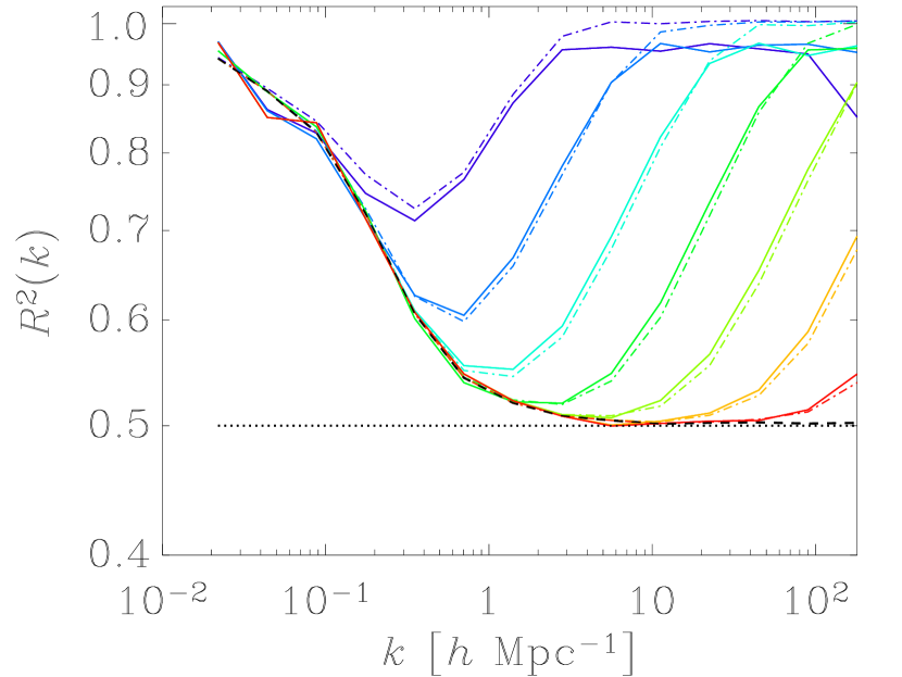
Figure 3: Testing eqs. (34) and (35) for $R^{2}(k)$. Density profiles $\rho(r)\sim r^{-2}$ were put around galaxies such that the central densities were held fixed, but the haloes grew in radius, proportional to their masses. The dotted line is at $1/\mu=0.5$, and the dashed curve is approximation (35). The solid curves depict $R^{2}$ for different halo radii per particle. The halo radius per particle varies by factors of $\sqrt{10}$ from $10^{-5.5}$ (rightmost upturn) to $10^{-2.5}{\ }h^{-1}{\,}{\rm Mpc}$ (leftmost upturn). For the set of haloes constructed with $10^{-2.5}{\ }h^{-1}{\,}{\rm Mpc}$ per particle, the minimum and maximum halo radii were 0.36 and $16{\ }h^{-1}{\,}{\rm Mpc}$. The dot-dashed curves show the approximations given by eqn. (34), with $(y_{gm}/y_{mm})^{2}$ calculated analytically.

We used the following procedure to separate the $1h$ and $2h$ terms of $\xi_{gm}$. First, Fourier-transform $\xi_{gm}$ and $\xi_{gg}$ [e.g. using FFTLog (Hamilton, 2000)], and then solve for $y_{gm}$ in eq. (26). To obtain $\xi_{gm}^{1h}$, Fourier-transform $P_{gm}^{1h}=y_{gm}^{1h}/n$ back into real space. Doing this requires an estimate of the large-scale bias $b_{0}$. If the size of the haloes is small compared to the volume of the sample, it is safe to assume that $y_{gm}(k_{\rm min})$ is of order unity, where $k_{\rm min}$ is the smallest wavenumber in the power spectrum. An upper limit, and quick estimate, of $b_{0}$ comes from assuming that $y_{gm}(k_{\rm min})=1$. If both $\xi_{gg}$ and $\xi_{gm}$ are measured well out to linear scales, $b_{0}$ may be measured directly from their ratio.

In Fig. 2, the full $1+\xi_{gm}$ overestimates the NFW profile by almost a factor of 2 at the largest scales, whereas $1+\xi_{gm}^{1h}$ reproduces it much better. The full and $1h$ $\xi_{gm}$’s start to diverge at about $r=0.7{\ }h^{-1}{\,}{\rm Mpc}$, which is the separation of the closest pair of galaxies, where $1+\xi_{gm}^{2h}$ starts to be positive. Our initial try of $y_{gm}(k_{\rm min})=1$ (giving $b_{0}=0.97$) subtracted off most of $\xi_{gm}^{2h}$, but using $y_{gm}(k_{\rm min})=0.8$ (giving $b_{0}=0.72$) resulted in a better fit. Thus, even though the halo diameters were only $1/16$ of the box size $l$, evidently $y_{gm}(k_{\rm min}=2\pi/l)$ did not quite reach unity.

5.1.2 Behaviour of the cross-correlation coefficient

This section describes a test of the galaxy-halo model approximations for the squared cross-correlation coefficient $R^{2}$, eqs. (34) and (35). We wanted to gauge the accuracy of the approximation, as well as investigate how halo profiles affect $R^{2}$ in general. For this test, the galaxy-halo profiles for all masses had a fixed density at each radius, but the truncation radius varied with mass. We used a convenient density profile, $\rho(r)\sim r^{-2}$, for which the truncation radius is proportional to mass.

For this test, the galaxy positions were those of the centres of the 4132 largest voboz haloes exceeding $2\sigma$ in the $256{\ }h^{-1}{\,}{\rm Mpc}$ simulation described above. The haloes ranged in mass from 230 to 10222, enough to give a dimensionless mean-square mass $\mu=2$. The smallest galaxy separation was $0.113{\ }h^{-1}{\,}{\rm Mpc}$.

Figure 3 shows the results of varying the halo radius per particle from $10^{-5.5}$ to $10^{-2.5}~{}{\ }h^{-1}{\,}{\rm Mpc}$. The power spectra $P_{gg}$, $P_{gm}$ and $P_{mm}$ were calculated from 3D FFTs of the galaxy and matter distributions, reaching small scales by ‘folding’ the particle distribution by factors of two (Klypin, private communication). For each fold, the boxes were split into eight octants, and each octant was superposed together in a box of half the size; thus, each fold enabled the FFT to reach scales smaller by a factor of two. At large scales, $R^{2}\approx 1$ because with a large window function, many galaxy haloes are averaged over. The $R^{2}$ curves then descend with $k$ as eq. (35) predicts, but then turn up at about the scale ($\pi/r$) of the largest halo radius, and finish ascending at about the scale of the smallest halo radius. It makes sense that $R^{2}\approx 1$ at small scales where the haloes are identical. Knowing everything about every halo makes it possible to calculate $y_{gm}/y_{mm}$ analytically; putting this into eq. (34) brought the approximation quite close to the measured $R^{2}$. For some reason, the measured $R^{2}$ curves did not quite reach unity, as the analytical curves would predict. Downturns, only visible here for the two largest halo radii per particle, occur at about the scale of the tightest matter pair. Such downturns would not occur in the real Universe, which has much higher ‘resolution.’

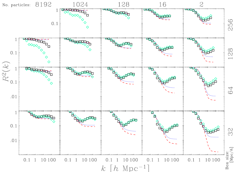
Figure 4: Testing approximation (35) for the galaxy-matter cross-correlation coefficient $R^{2}(k)$ in actual simulations, for different halo mass cut-offs and box sizes. From left to right, the halo mass (given in particle number) cut-off decreases by a factor of eight, the same factor by which the particle mass decreases from top to bottom with box size. Thus, the physical halo mass is the same along diagonals starting from the bottom-left and going up and right. The squares show $R^{2}$ calculated using only particles in haloes as identified by voboz, while the grey (online, green) diamonds show $R^{2}$ using all particles in the simulation. The dashed (online, red) lines show approximation (35), with the dimensionless mean-square halo mass $\mu$ calculated from the voboz halo masses. For the dotted (online, blue) lines, a smaller $\mu^{\prime}$ was used, calculated by identifying clusters of haloes (i.e. a halo and its subhaloes) such that each subhalo is within the half-mass radius of a parent halo, and then distributing the mass of the parent halo equally among the haloes and subhaloes. We fixed the large-scale bias $b_{0}$ by requiring that all of the curves line up in the largest-scale, lowest-wavenumber bin.

5.2 Simulations

The following tests involve more realistic density fields, drawn from simulations. The tests evaluate the galaxy-halo model’s descriptions of the cross-correlation coefficient and the bias between galaxies and matter.

5.2.1 The cross-correlation coefficient approximation

In this section, we discuss a comparison of the predictions of approximation (35) for the squared cross-correlation coefficient $R^{2}(k)$ with measurements from simulations. The test also investigates the degree to which it matters if orphans (particles not gravitationally bound to haloes) are included in the calculation. The galaxy positions were drawn from the centres of voboz-identified haloes in a suite of four $\Lambda$CDM simulations described by NHG.

Figure 4 shows $R^{2}$ for various halo catalogs, using different box sizes (32, 64, 128, and 256 ${\ }h^{-1}{\,}{\rm Mpc}$), and different lower mass thresholds. An additional threshold of $2\sigma$ in voboz halo probability eliminated many spurious haloes. Measurements of $R^{2}$, both including and excluding orphans (see sect. 4.3), are shown. Orphans make a significant difference in $R^{2}$ with a high halo mass threshold, but not otherwise. Orphans would likely make a greater difference if there were an upper mass threshold as well, since most of the pairs comprising $P_{gm}$ and $P_{mm}$ lie in the largest haloes.

Figure 4 also shows the approximation of eq. (35). For the dashed curves, we measured the dimensionless mean-square halo mass $\mu$ using the voboz particle halo membership. Some particles belong to more than one halo in voboz; we removed this ambiguity by assigning each particle to the smallest-mass voboz halo containing it.

In Fig. 4, especially for low mass thresholds, the $R^{2}$ curves do not reach their characteristic small-scale value as predicted from the voboz $\mu$. The dashed curves use a reduced $\mu^{\prime}$, in which the masses of haloes in clusters are equalized in an extreme way. (We define a cluster to be a set of haloes such that each halo is within the half-mass radius of another halo in the cluster.) For $\mu^{\prime}$, the mass of each halo in a cluster is set to the mass of the parent halo (the largest halo in the cluster) divided by the number of haloes in the cluster. This is not an unreasonable thing to do since, from the point of view of $R^{2}$, it may not be appropriate to distinguish between large parent haloes and small subhaloes. In a cluster environment, all $R^{2}$ sees is a group of galaxies surrounded by a bunch of matter; it does not know whether the matter is bound to parent haloes, to subhaloes, or to neither.

Figure 5 shows $\mu$ and $\mu^{\prime}$ as a function of lower halo mass cut-offs. As expected, the difference between them grows with the amount of substructure, i.e. as the halo mass cut-off is decreased. Figure 5 also shows $\mu_{\rm meas}$ as measured from the curves in Fig. 4; $\mu_{\rm meas}=1/R^{2}_{\rm min}$, where $R^{2}_{\rm min}$ is the lowest value $R^{2}(k)$ attains for $k<10{\ }h{\,}{\rm Mpc}^{-1}$. A simple fit to $\mu_{\rm meas}$ from our simulations, shown as the dotted curve in Fig. 5, is

$$\mu_{\rm meas}\approx 1+\left(\frac{M_{\rm min}}{10^{13}{\ }h^{-1}{\,}{\rm M_{\odot}}}\right)^{-0.4},$$ (39)

where $M_{\rm min}$ is the lower halo mass cut-off of the sample.

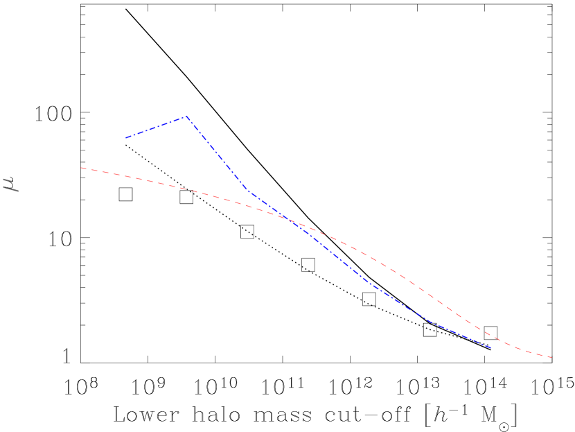
Figure 5: An illustration of different estimates of the dimensionless mean-square halo mass $\mu$ from four $\Lambda$CDM $N$-body simulations. The abcissa is the lower mass threshold used to define each halo sample. The curves are averages of the results from the four nested simulations. The positions of the squares show $\mu_{\rm meas}=1/R^{2}_{\rm min}$, where $R^{2}_{\rm min}$ is the lowest value $R^{2}(k)$ takes for $k<10{\ }h{\,}{\rm Mpc}^{-1}$, as measured from the $R^{2}(k)$ curves in Fig. 4. The solid curve shows $\mu$ as calculated from the voboz mass distributions. The (online, blue) dashdotted curve shows $\mu^{\prime}$, for which we reduced the dispersion by assigning all of the mass in clusters equally among their subhaloes. The dashed curve shows $\mu$ as calculated from the Sheth & Tormen (1999) mass function, using no upper mass threshold. The dotted line shows a crude fit to $\mu$, given in eq. (39). The height of the squares roughly indicates the scatter, which was similar in all curves. For very low and high mass cut-offs, the averages contained fewer than four samples because the cut-offs could not be used in all simulations.

The modified (in an extreme fashion) $\mu^{\prime}$ does agree with $\mu_{\rm meas}$ better than the original $\mu$, but there is still a significant difference, which can be explained with reference to Fig. 3. Galaxy-halo profiles encroach into the regime where $P_{gg}$ is significant, causing an upturn before (i.e. at larger scales than) $R^{2}$ would have attained its smallest value. Another way to look at the generic rise of $R^{2}$ at small scales is that, again referring to Fig. 3, the profiles of galaxy haloes of different masses are more similar to each other at small scales than at intermediate scales.

Figure 5 also shows an estimate of $\mu$ from a Sheth & Tormen (1999) mass function with a lower, but not upper, mass limit. This estimate agrees with $\mu_{\rm meas}$ about as well as the voboz $\mu$ estimate, except at high masses. We also tried estimating $\mu$ from the Sheth & Tormen (1999) mass function using an upper mass limit given by the largest halo mass appearing in each simulation. These results are not shown; this procedure estimated $\mu_{\rm meas}$ well for high-mass (and therefore low-substructure) halo samples in the $256{\ }h^{-1}{\,}{\rm Mpc}$ simulation, but somewhat poorly for lower-mass haloes in other simulations.

5.2.2 The bias approximation

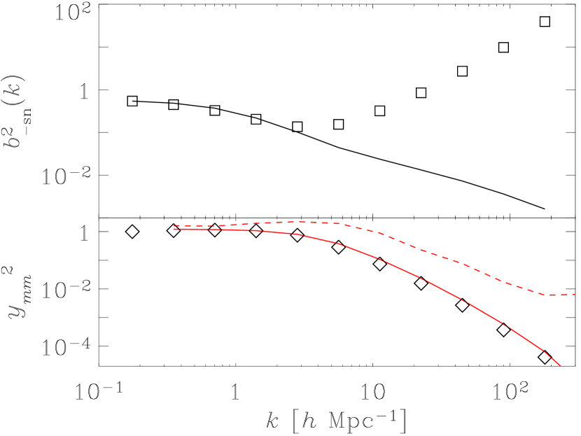
Figure 6: In the top panel, squares show the squared bias $b_{\rm-sn}^{2}(k)$ (excluding the shot noise from $P_{gg}$), and the curve shows the result of the galaxy-halo model, eq. (29), assuming that haloes are ‘infinitesimal nuggets’, i.e. that $y_{mm}(k)=1$. The value of the large-scale bias $b_{0}$ has been adjusted so that the squares and the curve in the top panel agree at the largest scale plotted. In the bottom panel, the diamonds show the ratio of the curve in the top panel to the squares; this ratio measures the mean-square average Fourier-transformed halo density profile $y_{mm}(k)^{2}$, assuming that $y_{mm}^{1h}=y_{mm}^{2h}$, as in eq. (29). For comparison, the grey (online, red) curves show $y_{mm}^{1h}(k)^{2}$ (solid) and $y_{mm}^{2h}(k)^{2}$ (dashed) from the same halo sample. (The square roots of these two latter curves appear in Fig. 1.)

Figure 6 shows the galaxy-matter bias $b_{\rm-sn}^{2}=P_{gg}/P_{mm}$ (excluding the shot noise from $P_{gg}$) as measured from a set of haloes taken from a $32{\ }h^{-1}{\,}{\rm Mpc}$ simulation (NHG), with a physical mass cut-off of $3\times 10^{10}{\ }h^{-1}{\,}{\rm M_{\odot}}$ (128 particles). On small scales, the measured bias increases relative to what the galaxy-halo model would predict if the haloes were infinitesimal nuggets of mass [i.e. that $y_{mm}(k)=1$ in eq. (29)]. This occurs because haloes are extended objects, i.e. because ${y_{mm}}^{2}$, the mean-square (weighting by the halo mass squared) halo profile, decreases from unity at small scales.

For this figure, we used the voboz estimate of the dimensionless mean-square halo mass $\mu=45$ (see the bottom middle panel of Fig. 4). The approximate concordance of the two quantities in the top panel reflects the fact that $y_{mm}$ is, as expected, near unity on large scales. To get the normalization of $P_{mm}$ right, it was necessary to divide by ‘orphan factors’ (see section 4.3) $(\rho_{h}/\rho)^{2}$, where $\rho$ is the total matter density, and $\rho_{h}$ is the density of matter in galaxy haloes. We fitted $b_{0}=0.27$ by requiring that the result of eq. (29), after dividing by $(\rho_{h}/\rho)^{2}$, equal the measured bias curve in the largest-scale bin. Including orphan factors, the effective large-scale bias becomes 0.75, rather small because the mass cut-off is low.

The bottom panel shows ${y_{mm}}^{2}$, the quotient between the measured bias and the infinitesimal-nugget prediction in eq. (29), along with measurements of $(y_{mm}^{1h})^{2}$ and $(y_{mm}^{2h})^{2}$. These would all lie on top of each other if the assumption that $y_{mm}^{1h}=y_{mm}^{2h}$ used for eq. (29) were true. For this set of haloes, $y_{mm}$ does not particularly trace the empirical $y_{mm}^{2h}$ [eq. (25)], but, conveniently, it does seem to follow the better-defined $y_{mm}^{1h}$ [eq. (22)]. This is not surprising, since the regime where $y_{mm}$ is interesting (i.e. not unity) is on small scales, where $P_{mm}^{1h}$ dominates $P_{mm}^{2h}$. At least in this case, the galaxy-halo model explanation of the bias rising on small scales because of an effective halo profile works plausibly well.

6 Interpreting observations

Increasingly sophisticated observations of weak gravitational lensing have recently led to high-signal-to-noise measurements of galaxy-matter clustering (Hoekstra et al., 2003; Sheldon et al., 2004). Measurements of the galaxy-matter correlation function $\xi_{gm}$ have previously been interpreted in at least two fashions: by direct comparison with haloes in dark-matter simulations such as the ones we have used (Tasitsiomi et al., 2004), and in the context of the halo model (Guzik & Seljak, 2002; Seljak et al., 2005a; Mandelbaum et al., 2005).

In this section, we illustrate how the galaxy-halo model can be used to extract information from measurements of $\xi_{gm}$ and $\xi_{gg}$; specifically, we use $\xi_{gm}$ (Sheldon et al., 2004) and $\xi_{gg}$ (Zehavi et al., 2002) as measured from a volume-limited sample of luminous Sloan Digital Sky Survey (SDSS) galaxies. Sheldon et al. and Zehavi et al. have also made more precise measurements from a larger, flux-limited sample, but they are harder to interpret, since the luminosity cut-off and galaxy number density change with redshift. On small scales where measurements exist for $\xi_{gm}$ but not for $\xi_{gg}$, we extrapolated $\xi_{gg}$ with a power law based on the two smallest-scale points. We also tried assuming $\xi_{gg}=0$ on small scales, which changed the results negligibly.

There are at least two ways to extract useful information from these observations with the galaxy-halo model. First, observations give the cross-bias $b(k)/R(k)$; with a model of the galaxy-matter cross-correlation coefficient $R(k)$, it is possible to measure the bias $b(k)$. Second, it is possible to extract an effective $\xi_{gm}^{1h}(r)$, or average overdensity profile $\bar{\delta}(r)$, of haloes around galaxies, as in Figure 2.

6.1 Measurement of bias

To measure the bias from the cross-bias $P_{gg}(k)/P_{gm}(k)=b(k)/R(k)$, it is necessary to estimate the cross-correlation coefficient $R(k)$. With a measurement of the bias, it is then possible to obtain the matter power spectrum. To get $R(k)$, it makes sense to use the simplest expression for $R(k)$ the galaxy-halo model has to offer, eq. (35). The most brazen assumption used for this equation is that $y_{gm}(k)=y_{mm}(k)$. As shown in Fig. 3, if halo profiles vary systematically with mass (which they almost certainly do in the real Universe), this assumption is valid only on scales larger than that of the largest halo. In simulations (Fig. 4), the approximation is good for $k\la 3{\ }h{\,}{\rm Mpc}^{-1}$, which makes sense since clusters have real-space sizes $\la 1{\ }h^{-1}{\,}{\rm Mpc}\approx\pi/(3{\ }h{\,}{\rm Mpc}^{-1})$. If an accurate model for $y_{gm}/y_{mm}$ is added, it would allow an accurate estimate of $R^{2}$ on smaller scales, using eq. (34).

Eq. (35) allows estimation of $R^{2}(k)$ with four ingredients: the galaxy power spectrum $P$, the galaxy number density $n$, a large-scale bias $b_{0}$, and the dimensionless mean-square halo mass $\mu$. The first two of these are known from the $\xi_{gg}$ measurement, but $\mu$ and $b_{0}$ are not.

Figure 5 suggests that the best way to estimate $\mu$ is to measure it from haloes in a simulation. We detected haloes with voboz in the same $256{\ }h^{-1}{\,}{\rm Mpc}$ simulation as used for Fig. 4 at redshift 0.1; the redshift of the observed sample varies between $0.1<z<0.174$. In a list of the haloes exceeding a $2\sigma$ probability threshold, the most massive 10028 haloes gave the same number density ($6\times 10^{-4}~{}h^{3}\,{\rm Mpc}^{-3}$) as the observed sample. The haloes ranged in particle number from 111 to 8364 (physically, from $9\times 10^{12}$ to $7\times 10^{14}{\ }h^{-1}{\,}{\rm M_{\odot}}$), giving $\mu=2.2$.

The correlation functions $\xi_{gg}$ and $\xi_{gm}$ from this simply defined set of haloes agree quite well with their observed counterparts. Previously, Tasitsiomi et al. (2004) compared the observed correlation functions to those of sets of haloes in their own simulations. Using a simple halo mass cut-off such as ours, their simulated correlation functions were significantly higher than the observations. However, by using a reasonable scatter in the mass-luminosity relation of dark matter haloes, they were able to lower the theoretical correlation functions to match the observations more closely. Such a ‘fuzzy’ halo mass cut-off lowered the correlation functions by allowing smaller-mass (and more weakly clustered) haloes into the sample. We do not fully understand why our correlation functions were lower (and thus able to reproduce the observations using a simple mass cut-off), but we suspect it might be explained largely from the small value of $\sigma_{8}=0.63$ used in our simulations.

It would be useful to estimate $\mu$ without taking the time to run and analyse a simulation. One alternative might be to estimate $\mu$ from a mass function (e.g. Sheth & Tormen, 1999). However, there is no reason to expect this to work perfectly, since the haloes in such a mass function are ‘largest virialized’ haloes as in the standard halo model. In Fig. 5, we show how well one attempt at estimating $\mu$ from this mass function works; it gives $\mu$ to within a factor of 2 or so. It may be possible to improve this guess by fixing an upper halo mass cut-off in addition to the lower mass cut-off we used. Another way to improve the $\mu$ estimate might come from, for example, combining a halo mass function, a subhalo mass function, and a halo occupation distribution, but with all of these ingredients, the galaxy-halo model would approach the complexity of the standard halo model.

What about the large-scale bias $b_{0}$? If $P_{gm}$ and $P_{gg}$ are measured well into the linear regime, where one is confident that $y_{gm}=1$, then $b_{0}$ may be measured directly from $P_{gm}=P/b_{0}+n^{-1}$. However, at present $P_{gm}$ is not measured to such large scales, so to analyze the present observations, it is necessary to make an educated guess for $b_{0}$.

Given the dimensionless mean-square halo mass $\mu$, putting $b_{0}=1/\mu$ in eq. (35) gives the largest-possible $R^{2}(k)$ at each $k$, giving

$$R^{2}_{b_{0}=1/\mu}=\frac{1/\mu+nP}{1+nP}.$$ (40)

The smallest-possible $R^{2}(k)$ occurs when $b_{0}\to\infty$ on large scales where $nP>1/\mu$, and when $b_{0}\to 0$ on small scales where $nP<1/\mu$. These minimum values of $R^{2}$ are

$$R^{2}_{b_{0}\to\infty} = [1+1/(nP)]^{-1};$$ (41)

$$R^{2}_{b_{0}\to 0} = [\mu(nP+1)]^{-1}.$$ (42)

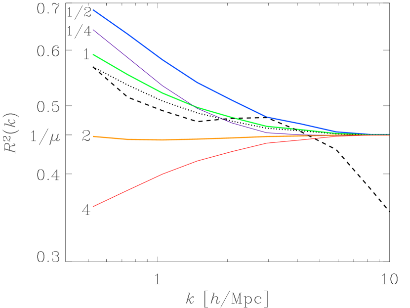
Figure 7: An illustration of how the galaxy-matter cross-correlation coefficient $R^{2}(k)$, calculated using eq. (35), depends on the large-scale bias parameter $b_{0}$. The galaxy spectrum $P$ is taken from from a volume-limited sample of luminous SDSS galaxies (Zehavi et al., 2002). The dimensionless mean-square halo mass $\mu$ is fixed at $2.2$. Solid curves are labelled according to the values of $b_{0}$ used to calculate them. For realistic halo samples, $b_{0}$ should seldom stray outside the range $1/2<b_{0}<2$; in extreme cases, it might venture out to $1/4$ or $4$. The curve at $b_{0}=1/2$ is nearly identical to the highest-possible $R^{2}(k)$ for each $k$, which uses $b_{0}=1/\mu\approx 0.45$. The dashed curve shows $R^{2}$ measured from a simulation described in the text. The dashed curve shows $R^{2}$ from eq. (35), using $b_{0}=1.12$, the value of $b_{0}$ which gives a curve matching the dashed curve in the lowest-wavenumber bin, at $k\approx 0.5{\ }h{\,}{\rm Mpc}^{-1}$.

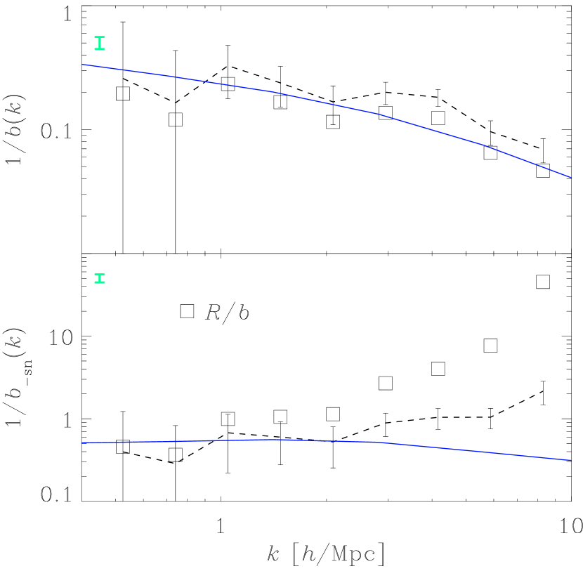
Figure 8: An attempt to measure the bias $b(k)$ (with the shot noise included in $P_{gg}$) and $b_{\rm-sn}(k)$ (without the shot noise in $P_{gg}$) of a volume-limited sample of luminous SDSS galaxies. Because the error bars are larger in $P_{gm}$, we put it in the numerator, showing $1/b$ instead of $b$. The squares show the cross-bias $R(k)/b(k)=P_{gm}(k)/P_{gg}(k)$, measured from $\xi_{gm}(r)$ (Sheldon et al., 2004) and $\xi_{gg}(r)$ (Zehavi et al., 2002). The dashed curves show $1/b$ as calculated by dividing $R/b$ by $R$ as calculated from eq. (35), and as shown in Fig. 7. For the dashed curves, we used a dimensionless mean-square halo mass $\mu=2.2$ and a large-scale bias $b_{0}=1.12$. The isolated, thick, grey (online, green) error bars in the upper-left corners of each panel show the largest fluctuation (in the smallest-wavenumber bin) in $1/b$ and $1/b_{\rm-sn}$ and if $b_{0}$ varies by factors of two in both directions from $1.12$. The thin, black error bars are the observational error bars, propagated through the analysis. The (online, blue) solid curves are $1/b$ measured from a halo catalog in a simulation; the halo catalog has a lower mass cut-off giving the same number density as the observed galaxy catalog.

Since in the present case, $P_{gm}$ is unavailable on confidently linear scales, the best way to get $b_{0}$ seems to be, again, to find it from a simulation. The $b_{0}$ we used comes from fitting eq. (35) to the actual $R^{2}(k)$ in the lowest-wavenumber bin, giving $b_{0}=1.12$. With no other information, a reasonable zeroth-order guess would be $b_{0}=1$.

Figure 7 shows how $R^{2}(k)$, as calculated with eq. (35), varies with $b_{0}$. It is unlikely that $b_{0}$ would wander by more than a factor of two or so from unity. In the lowest-wavenumber bin, $R$ varies only by a factor of $\sim 1.2$ as $b_{0}$ varies between $1/2$ and $2$. The measured $R^{2}$ from the simulation appears as the dashed curve.

Figure 8 shows the bias, both including and excluding the shot noise from $P_{gg}$, as inferred by dividing $R/b$ by $R$ from eq. (35). We plot $1/b$ instead of $b$ (as Sheldon et al. do) because the error bars are larger in $P_{gm}$ than in $P_{gg}$. The squares are the raw observations, $R/b$, and the dashed line shows the result after dividing this by $R$. In calculating $R$, $\mu=2.2$ and $b_{0}=1.12$ are fixed, but the thick error bars floating in the upper-left corners show the largest fluctuations (which occur at the largest scales) in $1/b_{\rm-sn}$ and $1/b$ if $b_{0}$ is multiplied and divided by 2.

The thin, larger error bars are the observational error bars in $1/b$, propagated through from $\xi_{gm}$ and $\xi_{gg}$. The error bars on $P_{gm}$, denoted $\delta P_{gm}$, are obtained by putting the covariance matrix of $\xi_{gm}$ (which Erin Sheldon kindly provided to us) through a two-dimensional FFTLog. Unfortunately, rigorous error bars have not been measured for $P_{gg}$ for this sample. As suggested by Idit Zehavi (private communication), we crudely estimated the error bars on $\xi_{gg}$ by assuming that in each bin, the fractional error $(\delta\xi_{gg})/\xi_{gg}$ is the same as that in the angular galaxy correlation function $(\delta w_{p})/w_{p}$, whose error bars have been measured. To estimate $\delta P_{gg}$, we put both $\xi_{gg}\pm\delta\xi_{gg}$ through FFTLog; we set $\delta\xi_{gg}=[F(\xi_{gg}+\delta\xi_{gg})-F(\xi_{gg}-\delta\xi_{gg})]/2$, where $F$ denotes a Fourier transform. The crudeness of $\delta P_{gg}$ is not terribly worrisome, though, since $(\delta P_{gm})/P_{gm}\gg(\delta P_{gg})/P_{gg}$.

The solid curves in Fig. 8 show the bias as measured from the simulation. There is good agreement between the dashed and solid curves on large scales, $k\la 3{\ }h{\,}{\rm Mpc}^{-1}$, where eq. (35) works reasonably well. It should be kept in mind that comparing the dashed to the solid curves tests not the galaxy-halo model, but how well the set of haloes chosen from the simulation represents the observed galaxies.

6.2 Measurement of average halo density profiles

Now we describe a measurement of an average halo density profile from these observations of $\xi_{gg}$ and $\xi_{gm}$; for a description of the procedure, see section 5.1.

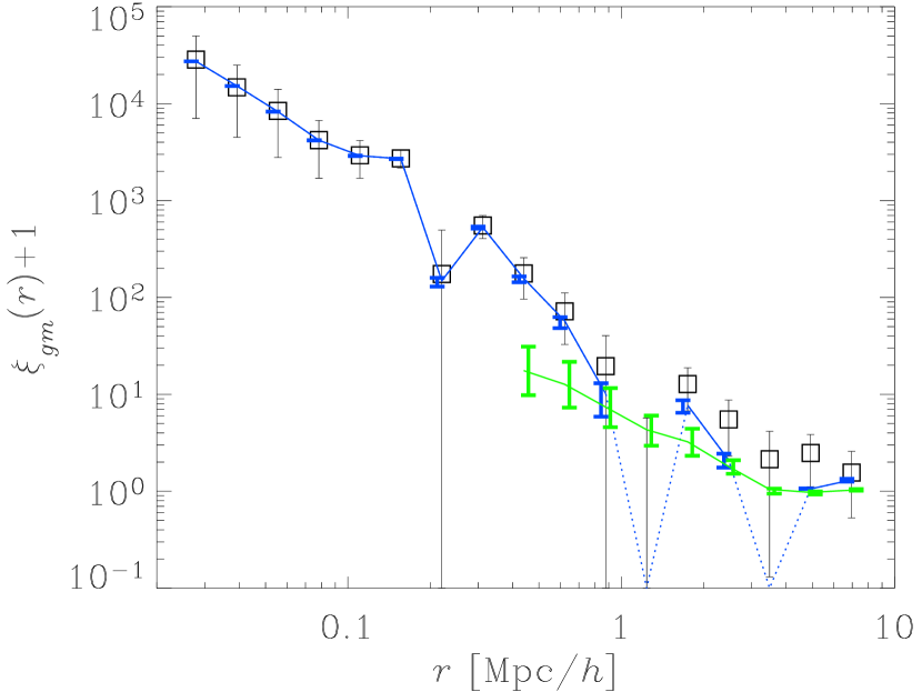
Figure 9: An attempt to recover the average overdensity profile of haloes around galaxies in a volume-limited sample of luminous SDSS galaxies from the galaxy-matter correlation function, using the galaxy correlation function. The squares with error bars are the measurement by Sheldon et al. (2004) of $\xi_{gm}$ (plus 1), and the dark grey (online, blue) solid curve is the effective one-halo term $\xi_{gm}^{1h}$, or $\bar{\delta}(r)$ (plus 1). This curve becomes dotted, and goes to the bottom of the plot, where $\xi_{gm}^{1h}+1<0$. The thick error bars around data points in the one-halo curve show the results of varying the large-scale bias $b_{0}$ by factors of 2 of the canonical value, $b_{0}=1.12$, in both directions. The light grey (online, green) curve is the two-halo term, $\xi_{gm}^{2h}+1$, again with thick error bars showing the fluctuation it experiences as $b_{0}$ changes by factors of 2.

Figure 9 shows a splitting of the observed galaxy-matter correlation function $\xi_{gm}$ into a one-halo term, $\xi_{gm}^{1h}=\bar{\delta}(r)$, and a two-halo term, $\xi_{gm}^{2h}$, calculated using the best-fitting $b_{0}=1.12$ from the previous section. The one-halo $\xi_{gm}^{1h}$ differs from the full $\xi_{gm}$ slightly on large scales, $r\ga 1{\ }h^{-1}{\,}{\rm Mpc}$. Evidently, there is not much overlap between haloes on the scales measured, which is not surprising since the high halo mass threshold precludes a large subhalo fraction in the sample. However, there is only a significant signal in $\xi_{gm}$ on scales $r\la 1{\ }h^{-1}{\,}{\rm Mpc}$, limiting the signal in $\xi_{gm}^{1h}$ and $\xi_{gm}^{2h}$ as well.

What does an ‘average halo profile’ really mean? In section 5.1, all of the halo profiles were identical (up to a multiplicative constant). In the real Universe, though, there are haloes of different sizes, shapes, and environments. The procedure in the present section gives the average halo profile under a partition of dark matter (including orphans) into haloes such that $y_{gm}^{1h}=y_{gm}^{2h}$. In such a partition, halo profiles do not depend systematically on the clustering of their galaxies. Although this equality holds fairly well in simulations, it cannot hold exactly, since in the real Universe, both halo profiles and the amplitude of the galaxy power spectrum depend on halo mass. However, the question remains: is it possible to partition the dark matter in the real Universe into ‘haloes’ around galaxies in a physically meaningful, if somewhat artificial, way to ensure that $y_{gm}^{1h}=y_{gm}^{2h}$? If there is, then our procedure to isolate the $1h$ and $2h$ terms of $\xi_{gm}$ gives the precise average halo profile if the dark matter is partitioned in this way.

7 Conclusion

This paper introduces a new, galaxy-halo model of large-scale structure. It is related conceptually to the standard halo model of large-scale structure, but there are significant differences. In the standard halo model, haloes are the fundamental objects; galaxies are placed within them according to the halo mass. In the galaxy-halo model, galaxies are the fundamental objects, which have (galaxy) haloes around them.

One result to come out of the galaxy-halo model is a deeper understanding of the galaxy-matter cross-correlation coefficient $R$ in terms of a halo mass dispersion. Equation (35), using a few inputs (the galaxy power spectrum, a large-scale bias, and a dimensionless measure of the scatter in the halo mass), gives an approximation for $R(k)$ which seems accurate on mildly non-linear scales, $k\la 3{\ }h{\,}{\rm Mpc}^{-1}$. With this model for $R$, it becomes feasible to measure the galaxy-matter bias down to scales $k\la 3{\ }h{\,}{\rm Mpc}^{-1}$ from measurements of the galaxy and galaxy-matter power spectra (or correlation functions), and thereby to infer the matter power spectrum down to these scales.

This equation for $R(k)$ has the following intuitive explanation. On small scales, the measurement of $R(k)$ samples at most one galaxy at a time. A scatter in halo mass thus naturally produces a scatter in the galaxy density-matter density relationship, producing a small value of $R(k)$ (this value depends on the spread in halo masses). On large scales, many haloes are averaged over to measure $R(k)$, reducing the scatter in the galaxy density-matter density relationship and forcing $R(k)$ toward unity.

The galaxy-halo model also provides a technique for inferring average halo density profiles, given measurements from a galaxy sample of the galaxy and galaxy-matter correlation functions. It is really the one-halo term of the galaxy-matter correlation function which corresponds to a average halo density profile; we present and test an algorithm to isolate this term.

Another application of the galaxy-halo model is to the bias $b^{2}(k)=P_{gg}(k)/P_{mm}(k)$ between galaxies and matter. If the shot noise is excluded from the galaxy power spectrum, the bias generally dips down on intermediate scales where the one-halo and two-halo terms of the matter power spectrum are comparable. On small scales, the bias generally increases with wavenumber because of haloes’ extended (not pointlike) density profiles, which cause a downturn in the matter power spectrum.

References

- Berlind & Weinberg (2002) Berlind, A.A., Weinberg, D.H., ApJ, 575, 587
- Coles (1993) Coles, P., MNRAS, 262, 1065
- Cooray & Sheth (2002) Cooray A., Sheth R., 2002, Phys. Rep., 372, 1
- Dekel & Lahav (1999) Dekel A., Lahav O., 1999, ApJ, 520, 24
- Guzik & Seljak (2002) Guzik J., Seljak U., 2002, MNRAS, 335, 311
- Hamilton (2000) Hamilton A.J.S., 2000, MNRAS, 312, 257
- Hamilton (2005) Hamilton A.J.S., 2005, to appear in Data Analysis in Cosmology, ed. V. Martínez, Springer-Verlag Lecture Notes in Physics (astro-ph/0503603)
- Hoekstra et al. (2003) Hoekstra H., van Waerbeke L., Gladders M.D., Mellier Y., Yee H.K.C., 2002, ApJ, 577, 604
- Ma & Fry (2000) Ma C., Fry J.N., 2000, ApJ, 543, 503
- Mandelbaum et al. (2005) Mandelbaum R., Tasitsiomi A., Seljak U., Kravtsov A.V., Wechsler R.H., 2005, MNRAS, submitted. (astro-ph/0410711)
- Mo & White (1996) Mo, H.J., White, S.D.M., 1996, 282, 347
- Navarro, Frenk & White (1997) Navarro J., Frenk C., White S., 1997, ApJ, 490, 493
- Neyman & Scott (1952) Neyman J., Scott E.L., 1952, ApJ, 116, 144
- Neyrinck, Hamilton & Gnedin (2004) Neyrinck M.C., Hamilton A.J.S., Gnedin N.Y., 2004, MNRAS, 341, 1 (NHG)
- Neyrinck, Gnedin & Hamilton (2005) Neyrinck M.C., Gnedin N.Y., Hamilton A.J.S., 2005, MNRAS, 356, 1222
- Peacock & Smith (2000) Peacock J.A., Smith R.E., 2000, MNRAS, 318, 1144
- Peebles (1980) Peebles P.J.E., 1980, The Large Scale Structure of the Universe. Princeton Univ. Press, Princeton
- Pen (1998) Pen, U., 1998, ApJ, 504, 601
- Scherrer & Bertschinger (1991) Scherrer R.J., Bertschinger E., 1991, ApJ, 381, 349
- Scoccimarro et al. (2001) Scoccimarro R., Sheth R.K., Hui L., Jain B., 2001, ApJ, 546, 20
- Seljak (2000) Seljak U., 2000, MNRAS, 318, 203
- Seljak & Warren (2004) Seljak U., Warren M.S., 2004, MNRAS, 355, 129
- Seljak et al. (2005a) Seljak U., et al., 2005a, Phys. Rev. D71, 043511
- Seljak et al. (2005b) Seljak U., et al., 2005b, Phys. Rev. D71, 103515
- Sheldon et al. (2004) Sheldon E.S. et al., 2004, AJ, 127, 2544
- Sheth & Tormen (1999) Sheth R.K., Tormen G., 1999, MNRAS, 308, 119
- Tasitsiomi et al. (2004) Tasitsiomi A., Kravtsov A.V., Wechsler R.H., Primack J.R., 2004, ApJ, 614, 533
- Tegmark & Bromley (1999) Tegmark M., Bromley B.C., 1999, ApJ, 518, L69
- Taruya & Soda (1999) Taruya A., Soda, J., 1999, ApJ, 522, 46
- Zehavi et al. (2002) Zehavi I. et al., 2002, ApJ, 571, 172