Searching for Transiting Planets in Stellar Systems

Abstract

We analyze the properties of searches devoted to finding planetary transits by observing simple stellar systems, such as globular clusters, open clusters, and the Galactic bulge. We develop the analytic tools necessary to predict the number of planets that a survey will detect as a function of the parameters of the system (age, extinction, distance, richness, mass function), the observational setup (nights observed, bandpass, exposure time, telescope diameter, detector characteristics), site properties (seeing, sky background), and the planet properties (frequency, period, and radius).

We find that for typical parameters, the detection probability is maximized for $I$-band observations. At fixed planet period and radius, the signal-to-noise ratio of a planetary transit in the $I$-band is weakly dependent on the mass of the primary for sources with flux above the sky background, and falls very sharply for sources below sky. Therefore, for typical targets, the number of detectable planets is roughly proportional to the number of stars with transiting planets with fluxes above sky (and not necessarily the number of sources with photometric error less a given threshold). Furthermore, for rising mass functions, the majority of the planets will be detected around sources with fluxes near sky. In order to maximize the number of detections, experiments should therefore be tailored such that sources near sky are above the required detection threshold. Once this requirement is met, the number of detected planets is relatively weakly dependent on the detection threshold, diameter of the telescope, exposure time, seeing, age of the system, and planet radius, for typical ranges of these parameters encountered in current transit searches in stellar systems. The number of detected planets is a strongly decreasing function of the distance to the system, implying that the nearest, richest clusters may prove to be optimal targets.

1. Introduction

Although radial velocity (RV) searches have provided an enormous amount of information about the ensemble properties of extrasolar planets, the interpretation of these results has been somewhat complicated by the fact that the planets’ properties have been shaped by the poorly-understood process of planetary migration. Short-period planets (periods $P\lesssim 10~{}{\rm days}$, i.e. “Hot Jupiters”) are essential for understanding this phenomenon, since they have all almost certainly reached their current positions via migration, and because they are the easiest to detect via several methods, including both radial velocities and transits. Thus, it is possible to rapidly acquire the statistics necessary for uncovering diagnostic trends in their ensemble properties, which may provide clues to the physical mechanisms that drive migration. Although RV searches have been and will continue to be very successful in detecting these planets, transit searches are rapidly gaining in importance.

There are currently over a dozen collaborations searching for planets via transits (see Horne 2003). These searches have recently started to come to fruition, and six close-in extrasolar giant planets have been detected using the transit technique to date (Konacki et al., 2003a; Bouchy et al., 2004; Pont et al., 2004; Konacki et al., 2004, 2005; Alonso et al., 2004), with many more likely to follow. Notably, transit searches have already uncovered a previously unknown population of “Very Hot Jupiters” – massive planets with $P\lesssim 3~{}{\rm days}$. Current transit searches can be roughly divided into two categories. Shallow surveys observe bright ($V\lesssim 14$) nearby stars with small aperture, large field-of-view dedicated instruments (Bakos et al., 2004; Kane et al., 2004; Borucki, et al., 2001; Pepper et al., 2004; Alonso et al., 2004; McCullough et al., 2004; Deeg et al., 2004). The goal of these surveys is primarily to find transiting planets around bright stars, which facilitate the extensive follow-up studies that are possible for transiting planets (Charbonneau et al., 2002; Vidal-Madjar et al., 2003, 2004; Charbonneau et al., 2005; Deming et al., 2005). On the other hand, deep surveys monitor faint $(V\gtrsim 14)$ stars using larger aperture telescopes with small field-of-view instruments. Typically, these searches do not use dedicated facilities, and thus are generally limited to campaigns lasting for a few weeks. In contrast to the shallow surveys, deep surveys will find planets around stars that are too faint for all but the most rudimentary reconnaissance. However, the primary advantage of these searches is that a large number of stars can be simultaneously probed for transiting planets. This allows such surveys to detect relatively rare planets, as well as probe planets in very different environments, and so robustly constrain the statistics of close-in planets. Deep searches can be further subdivided into two categories, namely searches around field stars in the Galactic plane (Udalski et al., 2002a, b, c, 2003, 2004; Mallén-Ornelas et al., 2003), and searches toward simple stellar systems.

Simple stellar systems, such as globular clusters, open clusters, and the Galactic bulge, are excellent laboratories for transit surveys, as they provide a relatively uniform sample of $\sim 10^{3-5}$ stars of the same age, metallicity, and distance. Furthermore, such surveys have several important advantages over field surveys. With minimal auxiliary observations, stellar systems provide independent estimates for the mass and radius of the target stars through main-sequence fitting to color-magnitude diagrams. An independent estimate for the stellar mass and radius, even with a crude transit light curve, can allow one to completely characterize the system parameters (assuming a circular orbit and a negligible companion mass). Transit data alone, without knowledge of the properties of the host stars, does not allow for breaking of the degeneracy between the stellar and planet radius and orbital semi-major axis. As a result, considerable additional expenditure of resources is required to confirm the planetary nature of transit candidates from field surveys (Dreizler et al., 2002; Konacki et al., 2003b; Pont et al., 2005a; Bouchy et al., 2005; Gallardo et al., 2005). Furthermore, using the results of field transit surveys to place constraints on the ensemble properties of close-in planets is hampered by a lack of information about the properties of the population of host stars, as well as strong biases in the observed distributions of planetary parameters relative to the underlying intrinsic planet population (Gaudi et al., 2004; Pont et al., 2005a; Gaudi, 2005; Dorsher et al., 2005). In contrast, the biases encountered in surveys toward stellar systems are considerably less severe, and furthermore are easily quantified because the properties of the host stars are known. This allows for accurate calibration of the detection efficiency of a particular survey, and so enables robust inferences about the population of planets from the detection (or lack thereof) of individual planetary companions (Gilliland et al., 2000; Weldrake et al., 2005; Mochejska et al., 2005; Burke et al., 2005).

There are a number of projects devoted to searching for transiting planets in stellar systems (Gilliland et al., 2000; Burke et al., 2003; Street et al., 2003; Bruntt et al., 2003; Drake & Cook, 2004; von Braun et al., 2005; Mochejska et al., 2005; Weldrake et al., 2005; Hidas et al., 2005). These projects have observed or are observing a number of different kinds of systems, with various ages, metallicities, and distances, using a variety of observing parameters, such as telescope aperture and observing cadence. Although several authors have discussed general considerations in designing and executing optimal surveys toward stellar systems (Janes, 1996; von Braun et al., 2005; Gaudi, 2000), these studies have been somewhat fractured, and primarily qualitative in nature. To date there has been no rigorous, quantitative, and comprehensive determination of how the different characteristics of the target system and observing parameters affect the number of transiting planets one would expect to find. To this end, here we develop an analytic model of transit surveys toward simple, homogeneous stellar systems. This model is useful for understanding the basic properties of such surveys, for predicting the yield of a particular survey, as well as for establishing guidelines that observers can use to make optimum choices when observing particular targets.

We concentrate on the simplest model that incorporates the majority of the important features of transit surveys toward stellar systems. We consider simple systems containing main-sequence stars of the same age and metallicity. We ignore the effects of weather, systematic errors (except at the most rudimentary level), and variations in seeing and background. Although we feel our analysis captures the basic properties of such searches without considering these effects, it is straightforward to extend our model to include these and other real-world effects.

In §2 we develop the equations and overall formalism that we use to characterize the detection probabilities of certain planets in specific systems with a given observational setup. In §3 we describe various analytic approximations we use to make sense of our detailed calculations, and we show how the transit detection probabilities depend on stellar mass and the characteristics of a particular survey. In §4 we list various physical relations and numerical approximations we use to calculate detection probabilities. In §5 we describe the dependence of the detection probabilities on the input parameters, and we present an application of our results in §6. We summarize and conclude in §7.

2. General Formalism

2.1. The Number of Detected Transiting Planets

For a given stellar system, the number of transiting planets with periods between $P$ and $P+dP$ and radii between $r$ and $r+dr$ that can be detected around stars with masses between $M$ and $M+dM$ is,

$$\frac{d^{3}N_{det}}{dMdrdP}=N_{*}f_{p}\frac{d^{2}p}{drdP}{\cal P}_{tot}(M,P,r)\frac{dn}{dM}.$$ (1)

Here, $N_{det}$ is the number of detected transiting planets; $N_{*}$ is the total number of stars in the system; $d^{2}p/drdP$ is the probability that a planet around a star in the system has a period between $P$ and $P+dP$ and a radius between $r$ and $r+dr$; $f_{p}$ is the fraction of stars in the system with planets; ${\cal P}_{tot}(M,P,r)$ is the probability that a planet of radius $r$ and orbital period $P$ will be detected around a star of mass $M$; and ${d}n/{d}M$ is the mass function of the stars in the system.

There are a number of assumptions that enter into equation (1):

• We assume that $f_{p}$ and $d^{2}p/drdP$ are independent of $M$. We normalize $d^{2}p/drdP$ to unity over a specific range of planetary radii and periods, and normalize $dn/dM$ to unity over a specific range of stellar masses. Therefore, $N_{*}$ is the number of (single) stars in the mass range of interest, and $f_{p}$ is the fraction of such stars harboring planets in the range of planetary radii and periods of interest. The number of such planets is thus $N_{p}=f_{p}N_{*}$, and the fraction that are detected is $f_{det}\equiv N_{det}/N_{p}$. The normalization of ${d}n/{d}M$ is described in §4.2, and the normalization of $d^{2}p/drdP$ is described in §4.6.

• We choose to use $P$ as our independent parameter rather than semi-major axis $a$, since it is the more directly observable quantity in transit searches, and it simplifies the following discussion considerably.

• We note that one of the primary simplifying assumptions in equation (1) is that all the target stars are at the same distance from the observer, which is an excellent assumption for most stellar systems.

2.2. Detection Probabilities ${\cal P}_{t}$, ${\cal P}_{W}$, ${\cal P}_{S/N}$

Following Gaudi (2000), we separate ${\cal P}_{tot}(M,P,r)$ into three factors

$${\cal P}_{tot}(M,P,r)={\cal P}_{t}(M,P){\cal P}_{S/N}(M,P,r){\cal P}_{W}(P),$$ (2)

where ${\cal P}_{t}$ is the probability that a planet transits its parent star, ${\cal P}_{S/N}$ is the probability that, should a transit occur during a night of observing, it will yield a Signal-to-Noise ratio (S/N) that is higher than some threshold value, and ${\cal P}_{W}$ is the window function which describes the probability that more than one transit will occur during the observations.

2.2.1 Transit Probability ${\cal P}_{t}$

The probability that a planet will transit its parent star is simply

$${\cal P}_{t}=\frac{R}{a}=\left(\frac{4\pi^{2}}{G}\right)^{1/3}M^{-1/3}RP^{-2/3}.$$ (3)

This form of ${\cal P}_{t}$ assumes that the planet is in a circular orbit. We will make this assumption throughout this paper.

2.2.2 Window Probability ${\cal P}_{W}$

The window function ${\cal P}_{W}(P)$ quantifies the probability that a planet with a given period $P$ will exhibit $n$ different transits during the times when observations are made. See Gaudi (2000) for a mathematical definition of ${\cal P}_{W}$. We will consider observational campaigns from single sites comprising a total of $N_{n}$ contiguous nights of length $t_{night}$. For an exploration of the effects of alternate observing strategies on ${\cal P}_{W}$, we refer the reader to a comprehensive discussion by von Braun et al. (2005). We will assume that no time is lost to weather. Finally, we require only that the center of the transit occurs during the night; therefore ${\cal P}_{W}$ depends only on $n$, $N_{n}$, $t_{night}$, and $P$, and does not depend on the transit duration. Note that our definition differs slightly from the definition by Mallén-Ornelas et al. (2003). In Figure (1), we show ${\cal P}_{W}$ as a function of $P$ for $N_{n}=10,20,40$ nights and $t_{night}=7.2$ hours, for the requirement of $n=2$ transits (which we will require throughout).

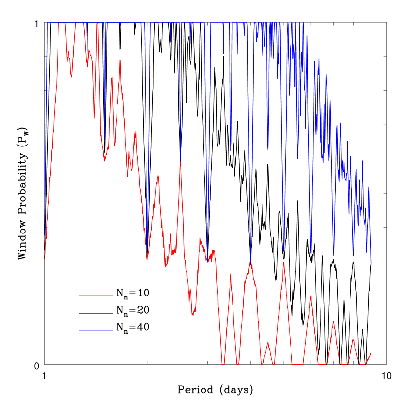
Figure 1.— The window probability ${\cal P}_{W}$, which is the probability that a planet with a given period will exhibit $n$ separate transits during the times observations are made. Here we have assumed 7.2 observable hours each night, that the run is $N_{n}$ nights long, and we have required $n=2$ transits to occur during the observing window. The lines show the results for $N_{n}=10$ (dotted), 20 (solid), and 40 (dashed).

2.2.3 Signal-to-Noise Probability ${\cal P}_{S/N}$

In this section, we determine ${\cal P}_{S/N}$, the probability that a single transit will exceed a ${\rm S/N}$ value larger than some minimum threshold ${\rm S/N}$ value. The signal-to-noise of a single transit is ${\rm S/N}=(\Delta\chi^{2})^{1/2}$, where $\Delta\chi^{2}$ is the difference in $\chi^{2}$ between a constant flux and a transit fit to the data. For simplicity, we will model all transits as boxcar curves. In this case, and under the assumption that only a small fraction of the data points occur during transit, the $\Delta\chi^{2}$ of a transit is simply,

$$\Delta\chi^{2}_{tr}=N_{tr}\left(\frac{\delta}{\sigma}\right)^{2}.$$ (4)

Here $N_{tr}$ is the number of observations during the transit, $\delta$ is the fractional change in the star’s brightness during the transit, and $\sigma$ is the fractional error of an individual flux measurement.

The number of observations $N_{tr}$ during a transit is related to the observing timescales: $N_{tr}=t_{tr}/(t_{read}+t_{exp})$, where $t_{tr}$ is the duration of the transit, $t_{read}$ is read time of the detector, and $t_{exp}$ is exposure time. We can put $t_{tr}$ in terms of the fundamental parameters:

$$t_{tr}=2x\sqrt{\frac{a}{GM}}=x\left(\frac{4P}{\pi GM}\right)^{1/3}.$$ (5)

Here, $x$ is half the length of the chord that traces the path of the transiting planet across the face of the star. Geometrically, $x=R\sqrt{1-b^{2}}$ where $b$ is the impact parameter of the transit. That is, $bR$ is equal to the distance from the equator to the latitude of the transit. For a transit with an inclination of $90$ degrees, $x=R$ and $b=0$, while for a grazing eclipse $x$ is nearly 0 and $b=1$. We define $t_{eq}$ as the duration of an equatorial transit (i.e. $t_{eq}=t_{tr}(b=0)$), and therefore $t_{tr}=t_{eq}\sqrt{1-b^{2}}$.

We assume a transit will be discovered if and only if $\Delta\chi^{2}_{tr}$ is larger than some threshold value $\Delta\chi^{2}_{min}$. We note that $\Delta\chi^{2}_{tr}=\Delta\chi^{2}_{eq}\sqrt{1-b^{2}}$. Therefore, the probability of achieving sufficient S/N is essentially a step function, such that:

$$\frac{d{\cal P}_{S/N}}{db}=\Theta\left[\Delta\chi_{eq}^{2}\sqrt{1-b^{2}}-\Delta\chi_{min}^{2}\right],$$ (6)

where $\Theta$ is the step function ($\Theta(x)=0$ for $x<0$; $\Theta(x)=1$ for $x\geq 0$). Equation (6) provides us with the probability that a transit with impact parameter between $b$ and $b+db$ will yield a sufficient S/N to be detected. This can be determined for a given set of intrinsic parameters of the system ($M,r,$ and $P$) and the observational parameters which we will list later.

We can assume that the impact parameters of transiting systems are distributed uniformly. We will take $b$ as our fundamental test of S/N, so that if a transit in a system with a given set of intrinsic parameters achieves sufficient S/N to be detected with an equatorial transit $b=0$, then it will be also detectable with any $b$ up to some inclination $b_{max}$, beyond which point it will not achieve sufficient S/N. We will integrate equation (6) from $b=0$ to $b_{max}$, which is the range over which ${\cal P}_{S/N}=1$:

$${\cal P}_{S/N}=\int_{0}^{1}\frac{d{\cal P}_{S/N}}{db}db=\int_{0}^{1}\Theta\left[\Delta\chi_{eq}^{2}\sqrt{1-b^{2}}-\Delta\chi_{min}^{2}\right]db\,.$$ (7)

This formulation makes it easy to eliminate the step function, since any argument with $b>b_{max}$ will cause the argument of the step function to be less than 0, and so the value of the integrand will equal 0. We can therefore integrate ${\cal P}_{S/N}$ from 0 to $b_{max}$, so the left hand side of equation (7) becomes

$${\cal P}_{S/N}=\int_{0}^{b_{max}}db=b_{max}\,.$$ (8)

We can take the right hand side of equation (7) and note that the argument of the step function will equal 0 when evaluated at $b_{max}$. Setting $\Delta\chi_{eq}^{2}\sqrt{1-b_{max}^{2}}-\Delta\chi_{min}^{2}=0$ and solving for $b_{max}$, we then have

$${\cal P}_{S/N}=b_{max}=\sqrt{1-\left(\frac{\Delta\chi^{2}_{min}}{\Delta\chi^{2}_{eq}}\right)^{2}}\,,\qquad{\rm if}\,\Delta\chi^{2}_{min}\leq\Delta\chi^{2}_{eq},$$ (9)

and ${\cal P}_{S/N}=0$ otherwise.

We must now determine the dependence of the various factors in equation (9) on the independent parameters $M,r,$ and $P$, as well as the observing parameters. Using equation (4), we can put $\Delta\chi_{eq}^{2}$ in terms of the independent parameters and $(\delta/\sigma)^{2}$. We must therefore relate $(\delta/\sigma)^{2}$ to the independent parameters. Assuming Poisson statistics, $\sigma=\sqrt{N_{S}+N_{B}}/N_{S}$, where $N_{S}$ is the number of photons recorded from a target star in a given exposure, and $N_{B}$ is the number of background photons. In terms of the observing parameters, $N_{S}=f_{\lambda}t_{exp}\pi(D/2)^{2}$, where $f_{\lambda}$ is the flux of photons with wavelength $\lambda$ from the target star, $D$ is the telescope aperture, and we have assumed a filled aperture. Flux is related to luminosity by

$$f_{\lambda}=\frac{L_{\lambda}}{4\pi d^{2}}10^{-A_{\lambda}/2.5},$$ (10)

where $L_{\lambda}$ is the star’s photon luminosity at wavelength $\lambda$, $A_{\lambda}$ is the interstellar extinction at wavelength $\lambda$, and $d$ is the distance to the system. Turning to the background sky photons, we can define

$$N_{B}=S_{sky,\lambda}\Omega t_{exp}\pi(D/2)^{2},$$ (11)

where $S_{sky,\lambda}$ is the photon surface brightness of the sky in wavelength $\lambda$ and $\Omega$ is effective area of the seeing disk.

Putting all this together, we can write $\Delta\chi^{2}_{eq}$ in terms of the parameters of the planet, primary, and observational setup,

$$\Delta\chi^{2}_{eq}=(1024\pi)^{-1/3}\frac{t_{exp}}{t_{read}+t_{exp}}\left(\frac{r}{R}\right)^{4}\left(\frac{D}{d}\right)^{2}\left(\frac{PR^{3}}{GM}\right)^{1/3}L_{\lambda}10^{-0.4A_{\lambda}}\left(1+\frac{S_{sky,\lambda}\Omega 4\pi d^{2}}{L_{\lambda}10^{-0.4A_{\lambda}}}\right)^{-1}.$$ (12)

This form can then be inserted into equation (9) to find ${\cal P}_{S/N}$.

Note that we have assumed Poisson statistics, no losses due to the atmosphere, telescope, or instrumentation, and no additional background flux other than that due to sky (no blending). In §4.3, we introduce a systematic floor to the photometric error $\sigma$. However, other than this one concession to reality, our results will represent the results of ideal, photon-limited experiments, and are therefore in some sense the best case outcomes. When designing actual experiments, such real-world complications need to be considered carefully to ensure that they do not substantially alter the conclusions drawn here.

3. Analytic Approximations - Sensitivity as a Function of Primary Mass

To lowest order, the main-sequence population of a coeval, homogeneous stellar system forms a one-parameter system of stars. Therefore, a novel aspect of transit searches in stellar systems is that, once the cluster, planet, and observational parameters have been specified, the sensitivity of different stars can be characterized by a single parameter, namely the stellar mass. This simple behavior, combined with assumptions about the mass-luminosity relation, mass-radius relation, and mass function, allows us derive analytic results for the sensitivity of transit surveys as a function of stellar mass.

Here we consider the sensitivity of a given transit search to planets of a given radius $r$ and period $P$ as a function of the primary mass $M$. Adopting power-law forms for the mass-luminosity and mass-radius relations, we rewrite the analytic detection probabilities for ${\cal P}_{t}$ and ${\cal P}_{S/N}$ that we derived in §2.2 in terms of $M$. We note that, due to the manner in which we have defined it, ${\cal P}_{W}$ depends only on $P$ and the observational parameters, and not on $M$. This simplifies the understanding of the sensitivity considerably, since ${\cal P}_{W}$ is the only factor that must be calculated numerically.

3.1. Mass-Luminosity and Mass-Radius Relations

We adopt generic power-law mass-luminosity and mass-radius relations,

$$R=R_{\odot}\left(\frac{M}{M_{\odot}}\right)^{\alpha},\qquad L_{\lambda}=L_{\lambda,\odot}\left(\frac{M}{M_{\odot}}\right)^{\beta_{\lambda}}$$ (13)

where $L_{\lambda,\odot}$ is the photon luminosity at a wavelength $\lambda$ for a solar-mass star. The power-law index for the mass-luminosity relation is wavelength-dependent, such that the $\beta_{\lambda}$ index accounts for bolometric corrections for particular bandpasses.

We note that neither empirically calibrated nor theoretically predicted mass-radius and mass-luminosity relations are strict power laws. However, the power-law relations lead to useful analytic results that aid in the intuitive results of the more precise results presented later. Furthermore, for stars near $M\sim M_{\sun}$ and optical bandpasses, this approximation is reasonably accurate.

For the most part, we will keep the resulting analytic expressions in terms of the variables $\alpha$ and $\beta_{\lambda}$, rather than substitute specific values. However, as will become clear, some interesting properties of these expressions are seen for realistic values of these parameters. Therefore, where appropriate, we occasionally insert numerical values for $\alpha$ and $\beta_{\lambda}$. As we show later, for most targets, the $I$-band proves to be optimal in terms of maximizing the signal-to-noise ratio of detected transits. For the $I$-band, and $0.3~{}M_{\odot}\lesssim M\lesssim 2M_{\odot}$, typical values are $\alpha=1$ and $\beta_{I}=3.5$.

3.2. Dependence of ${\cal P}_{S/N}$ on $M$

We first consider $\Delta\chi^{2}_{eq}$ and ${\cal P}_{S/N}$. Substituting equation (13) into equations (9) and (12), we find after some algebra,

$$\frac{\Delta\chi^{2}_{eq}}{\Delta\chi^{2}_{min}}=\frac{1}{C_{1}}\left(\frac{M}{M_{\odot}}\right)^{-(3\alpha-\beta_{\lambda}+1/3)}\left[1+C_{2}\left(\frac{M}{M_{\odot}}\right)^{-\beta_{\lambda}}\right]^{-1}$$ (14)

$${\cal P}_{S/N}=\left\{1-C_{1}^{2}\left(\frac{M}{M_{\odot}}\right)^{2(3\alpha-\beta_{\lambda}+1/3)}\left[1+C_{2}\left(\frac{M}{M_{\odot}}\right)^{-\beta_{\lambda}}\right]^{2}\right\}^{1/2}$$ (15)

where we absorb all the constants and parameters except for mass into the new constants $C_{1}$ and $C_{2}$, which are given by,

$$C_{1}=(1024\pi)^{1/3}\Delta\chi^{2}_{min}\left(1+\frac{t_{read}}{t_{exp}}\right)\left(\frac{r}{R_{\odot}}\right)^{-4}\left(\frac{d}{D}\right)^{2}\left(\frac{GM_{\odot}}{PR_{\odot}^{3}L_{\lambda,\odot}^{3}}\right)^{1/3}10^{0.4A_{\lambda}},$$ (16)

$$C_{2}=\frac{4\pi d^{2}S_{sky,\lambda}\Omega}{L_{\lambda,\odot}10^{-0.4A_{\lambda}}}.$$ (17)

Note that $C_{2}$ is simply the ratio of the flux in the seeing disk to the flux of a star of $M_{\odot}$.

Inspection of the behavior of equation (15) as a function of $M$ reveals that there are two different regimes. In the first regime the second term within the square brackets is much smaller than unity and hence negligible. This is the regime in which the photon noise is dominated by the source (i.e. the target star). In the opposite regime, where that term is much larger than unity, the noise is dominated by the sky background. The transition between these two regimes occurs at the mass $M_{sky}$ where the flux from the star is equal to the flux from the sky background,

$$M_{sky}=C_{2}^{1/\beta_{\lambda}}M_{\odot}.$$ (18)

The behavior of ${\cal P}_{S/N}$ as a function of mass depends on the value of $\Delta\chi^{2}_{eq}/\Delta\chi^{2}_{min}$ at $M=M_{sky}$. If $\Delta\chi^{2}_{eq}/\Delta\chi^{2}_{min}<1$ at $M=M_{sky}$, then the ability to detect planets is limited by the source noise for all the stars in the system. Conversely, if $\Delta\chi^{2}_{eq}/\Delta\chi^{2}_{min}>1$ at $M=M_{sky}$, then the ability to detect planets around the faintest stars in the system is limited by noise due to the sky background. That is to say, a particular experiment can be characterized by whether the flux of the faintest star around which a planet can be detected is brighter or dimmer than the sky. We call these the “source limited” and “background limited” regimes, respectively. We shall see the implications of this distinction shortly. An experiment is in the background limited regime when $\Delta\chi^{2}_{eq}/\Delta\chi^{2}_{min}\geq 1$ for $M\geq M_{sky}$, which implies,

$$2C_{1}C_{2}^{(3\alpha-\beta_{\lambda}+1/3)/\beta_{\lambda}}\leq 1.$$ (19)

In the source noise limited regime, we find that

$$\frac{\Delta\chi^{2}_{eq}}{\Delta\chi^{2}_{min}}=\frac{1}{C_{1}}\left(\frac{M}{M_{\odot}}\right)^{-(3\alpha-\beta_{\lambda}+1/3)},\qquad{\rm(Source~{}Limited)},$$ (20)

where ${\cal P}_{S/N}$ becomes

$${\cal P}_{S/N}\simeq\left[1-C_{1}^{2}\left(\frac{M}{M_{\odot}}\right)^{2(3\alpha-\beta_{\lambda}+1/3)}\right]^{1/2},\qquad{\rm(Source~{}Limited)}.$$ (21)

On the other hand, in the background noise limited regime,

$$\frac{\Delta\chi^{2}_{eq}}{\Delta\chi^{2}_{min}}=\frac{1}{C_{1}C_{2}}\left(\frac{M}{M_{\odot}}\right)^{-(3\alpha-2\beta_{\lambda}+1/3)},\qquad{\rm(Background~{}Limited)},$$ (22)

and

$${\cal P}_{S/N}\simeq\left[1-(C_{1}C_{2})^{2}\left(\frac{M}{M_{\odot}}\right)^{2(3\alpha-2\beta_{\lambda}+1/3)}\right]^{1/2},\qquad{\rm(Background~{}Limited)}.$$ (23)

Both of these equations have the same general form. For masses below a certain threshold, $M_{th}$, there is no chance of detecting a transit. The formula for $M_{th}$ can be determined separately for the two different noise regimes. In the source noise limited regime, we have

$$M_{th,s}=\left(C_{1}\right)^{-1/(3\alpha-\beta_{\lambda}+1/3)}M_{\odot},$$ (24)

while in the background noise limited regime,

$$M_{th,b}=\left(C_{1}C_{2}\right)^{-1/(3\alpha-2\beta_{\lambda}+1/3)}M_{\odot}.$$ (25)

Thus ${\cal P}_{S/N}$ as a function of stellar mass is approximately a step function, and the placement of the step, $M_{th}$ will depend on whether the faintest star around which a planet is detectable (for which $\Delta\chi^{2}_{eq}>\Delta\chi^{2}_{min}$) is brighter or dimmer than the sky. Although the labels “source limited” and “background limited” refer to the faintest star for which a planet is detectable, and not to all the stars in the system, we shall see shortly that the integrated detection probability will depend primarily on the lowest-mass stars.

It is highly instructive to insert numerical values for $\alpha$ and $\beta_{\lambda}$ and consider the behavior of $\Delta\chi^{2}_{eq}$ and ${\cal P}_{S/N}$ in the source and background limited regimes. Adopting values appropriate to the $I$-band, ($\alpha=1$ and $\beta_{I}=3.5$), we have $3\alpha-\beta_{\lambda}+1/3=-1/6$, and thus $\Delta\chi^{2}_{eq}\propto M^{1/6}$ in the source-noise limited regime. Thus, for sources above sky, the signal-to-noise is an extremely weak function of mass. On the other hand, for sources below sky, we have that $3\alpha-2\beta_{\lambda}+1/3=-11/3$, and thus $\Delta\chi^{2}_{eq}\propto M^{11/3}$, an extremely strong function of mass. Taken together, these results imply that, if it is possible to detect transiting planets around any stars in the target system, it is possible to detect planets with the same radius and period around all stars in the system above sky. For stars fainter than sky, the detection rapidly becomes impossible with decreasing mass. These effects are illustrated in §5.1.

These results have an interesting corollary that informs the experimental design. If the experiment is background limited (i.e. $\Delta\chi^{2}_{eq}(M_{sky})\geq\Delta\chi^{2}_{min}$), then the minimum stellar mass around which a planet is detectable is $M_{th,b}/M_{\odot}=(C_{1}C_{2})^{3/11}$, whereas in the source limited regime $M_{th,s}/M_{\odot}=(C_{1})^{6}$. Since the constants $C_{1}$ and $C_{2}$ depend on the parameters of the target system, the experimental setup, and the observational parameters, these scaling relations generally imply that the yield of experiments in the background limited regime is relatively insensitive to the precise values of these parameters, whereas the opposite is true for experiments in the source limited regime. Said very crudely: specific experiments are either capable of detecting planets or they are not. Experiments should be tailored such that $\Delta\chi^{2}_{eq}/\Delta\chi^{2}_{min}\geq 1$ at $M=M_{sky}$, which implies that $2C_{1}C_{2}^{(3\alpha-\beta_{\lambda}+1/3)/\beta_{\lambda}}\leq 1$, but provided this requirement is well-satisfied, changing the observational parameters will have little effect on the number of detected planets.

3.3. Dependence of ${\cal P}_{t}$ on $M$

We next consider ${\cal P}_{t}$. Substituting equation (13) into equation (9) and (12),

$${\cal P}_{t}=C_{3}\left(\frac{M}{M_{\odot}}\right)^{\alpha-1/3},$$ (26)

where we have defined

$$C_{3}=\left(\frac{4\pi^{2}R_{\odot}^{3}}{P^{2}GM_{\odot}}\right)^{1/3}=0.238\left(\frac{P}{\rm day}\right)^{-2/3}.$$ (27)

3.4. Dependence of $dn/dM$ on $M$

We assume a differential mass function of the form

$$\frac{dn}{dM}\equiv k\left(\frac{M}{M_{\odot}}\right)^{\gamma}.$$ (28)

The constant $k$ must be chosen such that that the integral over $dn/dM$ is equal to unity, i.e. such that

$$\int^{M_{max}}_{M_{min}}dMk\left(\frac{M}{M_{\odot}}\right)^{\gamma}=1\,,$$ (29)

where $M_{max}$ and $M_{min}$ are the masses of the largest and smallest stars in the system to be considered. Solving equation (29) for $k$ gives us $k=(\gamma+1)M_{\odot}^{\gamma}/[M_{max}^{\gamma+1}-M_{min}^{\gamma+1}]$.

3.5. Dependence of ${\cal P}_{tot}(dn/dM)$ on $M$

We can now use these forms for ${\cal P}_{S/N}$ and ${\cal P}_{t}$, together with assumptions about the mass function of the stellar system $dn/dM$, to evaluate the detection sensitivity to planets with a given set of properties.

To a first approximation, ${\cal P}_{S/N}$ is simply a step function such that ${\cal P}_{S/N}=\Theta(M-M_{th})$, where $M_{th}$ is the minimum threshold mass. This is given by $M_{th}=M_{th,b}$ if $\Delta\chi^{2}(M_{sky})\geq\Delta\chi^{2}_{min}$, and $M_{th}=M_{th,b}$ otherwise. Thus for masses $M\geq M_{th}$, the sensitivity as a function of mass is dominated by the effects of ${\cal P}_{t}$ and $dn/dM$. We can write

$${\cal P}_{tot}(M,P,r)\frac{dn}{dM}={\cal P}_{W}(P)C_{3}(P)k\left(\frac{M}{M_{\odot}}\right)^{\zeta}\Theta(M-M_{th}).$$ (30)

where $\zeta\equiv\alpha-1/3+\gamma$. For a Saltpeter slope of $\gamma=-2.35$, and $\alpha=1$, $\zeta\simeq-1.68$. Therefore, under the assumption that the frequency of planets of a given radius and period is independent of the mass of the primary, the number of detected planets is dominated by parent stars with mass near $M_{th}$, which, in the usual case of a background-dominated experiment, is for stars with flux just below the sky.

4. Additional Ingredients

In §3 we adopted several simplifying assumptions and approximations that allowed us to derive analytic expressions for the detectability of planets as a function of primary mass. Inspection of these expressions allowed us to infer some generic properties of transit searches in stellar systems. However, in order to make realistic estimates of the number of planets a particular survey will detect, here we add a few additional ingredients to the basic formalism presented in §2. We will also present a somewhat more sophisticated treatment of the mass-luminosity relation, as well as adopt specific values for several parameters as necessary to make quantitative predictions.

4.1. Reconsidering the Mass-Luminosity Relation

The above analysis approximated the mass-luminosity relation as a simple power law in each wavelength band. As we have already discussed, this assumption is incorrect in detail. We therefore provide a somewhat better approximation to the mass-luminosity relation. We analytically relate $L_{\lambda}$ to $L_{bol}$, assuming purely blackbody emission, and that the bolometric mass-luminosity relation can be expressed as a power law:

$$L_{bol}=L_{{bol},\odot}\left(\frac{M}{M_{\odot}}\right)^{\beta},$$ (31)

in which $\beta$ is a single number – the bolometric power law index – instead of the wavelength-dependent index $\beta_{\lambda}$ in equation (13). Empirically, this is known to be a reasonable approximation for $0.3M_{\odot}\lesssim M\lesssim 2M_{\odot}$ (Popper, 1980). We combine this bolometric relation with the mass-radius relation from equation (13), and with $L_{bol}=4\pi R^{2}\sigma T^{4}$. We can then write temperature as a function of mass,

$$T(M)=T_{\odot}\left(\frac{M}{M_{\odot}}\right)^{(\beta-2\alpha)/4},\qquad T_{\odot}=\left(\frac{L_{bol,\odot}}{4\pi\sigma R_{\odot}^{2}}\right)^{1/4},$$ (32)

where $T_{\odot}=5777~{}{\rm K}$ is the effective temperature of the sun. We can write the luminosity of a blackbody in a particular band $X$ as:

$$L_{X}(T)=\int^{+\infty}_{-\infty}{\cal T}_{X}(\lambda^{\prime})B_{\lambda^{\prime}}(T)(4\pi R^{2})(\pi)d\lambda^{\prime},$$ (33)

where $B_{\lambda}(T)$ is the Planck law per unit wavelength, and ${\cal T}_{X}(\lambda)$ is the transmission for filter X. We can approximate this formula by assuming that the transmission ${\cal T}_{X}(\lambda)$ of filter $X$ is a simple top hat with unit height, effective width $\Delta\lambda_{X}$, and effective wavelength $\lambda_{c,X}$. We can also replace the integral with a product, since $B_{\lambda}(T)$ does not change significantly over the intervals defined by the visible or near-infrared filters we will be considering. Also, we can use equation (32) to write $L_{X}$ as a function only of mass. Thus, we can rewrite equation (33) as

$$L_{X}(M)=\frac{8\pi^{2}cR^{2}\lambda_{c,X}^{-4}\Delta\lambda_{X}}{\exp\left(\frac{hc}{\lambda_{c,X}kT(M)}\right)-1}\,.$$ (34)

To check this form of the luminosity function, we compare its reported luminosities to those from the Yale-Yonsei (${\rm Y}^{2}$) isochrones (Yi et al., 2001), which use the Lejeune, Cuisinier, & Buser (1998) color calibration. We find that this form for $L_{X}(M)$ is sufficiently accurate for our purposes. In particular, it is much more accurate than the simple power-law approximations we considered in §3. Nevertheless, we find that the qualitative conclusions outlined in that section still holds using the more accurate form for the mass-luminosity relation, and thus we can still use the intuition gained by studying the behavior predicted by the analytic approximations derived in §3 to guide our interpretation of the results presented in the rest of the paper.

4.2. Normalizing the Mass Function

To normalize the mass function, we need to determine which values to use for $M_{min}$ and $M_{max}$, which are used to compute the normalization constant $k$. We should choose values that limit the set of stars in the analysis to those around which planets are likely to be detected.

Somewhat anticipating the results from the following sections, we will set $M_{min}=0.3M_{\odot}$ for our fiducial calculations. This represents the lowest mass star around which a planet can be detected, for typical ranges of the observational, system, and planet parameters encountered in current transit searches. In some cases, it may be possible to detect planets around stars of lower mass. On the other hand, one might be interested in only those stars for which precise radial velocity follow-up is feasible for 8m-class telescopes. Therefore, in §5.4, we consider the effects of varying $M_{min}$ on the number of detectable planets.

We set $M_{max}$ to be the most massive main sequence star in the system, i.e. a turnoff star. We determine the mass of a turnoff star, $M_{to}$, using the simple relation $L_{bol,to}=\epsilon M_{to}c^{2}/A$, where $\epsilon$ is the net efficiency of hydrogen burning ($\epsilon=0.00067$) and $A$ is the age of the target system. Combining this expression with the bolometric mass-luminosity relation from equation (31) gives us

$$M_{to}=\left(\frac{\epsilon M_{\odot}^{\beta}c^{2}}{L_{bol,\odot}A}\right)^{1/(\beta-1)}.$$ (35)

4.3. Minimum Observational Error

In §2.2.3, we calculate $\sigma$ using a formula for pure photon noise errors. In real observations, photometric errors do not get arbitrarily precise for a given source and background. Therefore, we impose a minimum systematic observational error of $\sigma_{sys}=0.1\%$ to mimic the practical difficulties of obtaining precise observations of bright stars. The calculated errors therefore become equal to $\sigma=\left(\sigma_{phot}^{2}+\sigma_{sys}^{2}\right)^{1/2}$, where $\sigma_{phot}$ is the photon-noise error.

4.4. Effective Area of the Seeing Disk

We assume the point-spread function (PSF) is a Gaussian with a full-width half-maximum of $\theta_{see}$, which has an effective area of,

$$\Omega=\frac{\pi}{\ln 4}\theta_{see}^{2}.$$ (36)

4.5. Saturation Mass

Detectors have a finite dynamic range, and we clearly cannot detect planets around saturated stars. When integrating over mass, we therefore ignore stars with $M\geq M_{sat}$, where $M_{sat}$ is the mass of a star that just saturates the detector. We assume that a star saturates the detector when the number of photons $N_{phot}$ from the star and sky that fall into the central pixel of the stellar PSF exceeds the full well depth of a pixel, $N_{FW}$. We approximate $N_{phot}$ as,

$$N_{phot}=\left(f_{\lambda}\left\{1-\exp\left[-\ln 2\left(\frac{\theta_{pix}}{\theta_{see}}\right)^{2}\right]\right\}+S_{sky,\lambda}\theta_{pix}^{2}\right)t_{exp}\pi\left(\frac{D}{2}\right)^{2},$$ (37)

where $\theta_{pix}$ is the angular size of a single pixel. This form assumes a Gaussian PSF perfectly centered on the central pixel. The assumption of Gaussian PSF is reasonable for our purposes, and the assumption that the PSF is centered on a pixel conservatively underestimates $M_{sat}$. Formally, equation (37) only holds for circular pixels, but is nevertheless accurate to $\lesssim 20\%$ for square pixels. This is sufficient for our purposes.

4.6. Planet Distribution

To compute the number of detected planets, we integrate $d^{3}N_{det}/drdPdM$ (see equation (1)) over $M$, $P$, and $r$ to find $N_{det}$. We therefore must assume a form for the distribution of planets, $d^{2}p/drdP$. We will assume that the periods are distributed evenly in log space, as is suggested by several analyses (e.g., Tabachnik & Tremaine 2002). Since radii have been measured for only seven planets, the distribution of the radii is very poorly known. We will therefore simply assume a delta function at $r=r^{\prime}$, and adopt $r^{\prime}=0.1R_{\odot}$ for our fiducial calculations. However, we will also explore the detectability as a function of $r$. Our adopted distribution of periods and radii can therefore be expressed as,

$$\frac{d^{2}p}{drdP}=\frac{1}{\Delta\ln P}P^{-1}\delta(r-r^{\prime})\,,$$ (38)

where $\Delta\ln P$ is the logarithmic range of periods of interest.

From a comparison of the results from radial velocity and transit surveys, it appears that there are two distinct populations of close-in massive planets. “Very Hot Jupiters” have periods between $1-3~{}{\rm days}$, and are approximately ten times less common than “Hot Jupiters” with periods between $3-9~{}{\rm days}$ (Gaudi et al., 2004). We will therefore consider these two ranges of periods separately.

4.7. Extinction

We consider two models for the extinction. In general, we assume an extinction of a fixed value $A_{I}$ in the $I$-band, and calculate the extinction in the other bands using the extinction ratios listed in Table 2. We also consider an extinction that depends on the distance to the stellar system as,

$$A_{I}(d)=0.5~{}{\rm mag}\left(\frac{d}{\rm kpc}\right)\,,$$ (39)

where we again use the the extinction ratios in Table 2 to determine the extinction in the other bands. We use the fixed-extinction law in all calculations and plots unless otherwise specified.

4.8. Fiducial and Fixed Parameters

There are a number of parameters in these equations for which we must assign values. In §5.3 we will examine the dependence of the detection probabilities on a subset of the most interesting of these parameters. These include the cluster distance $d$, age $A$, mass function slope $\gamma$, and extinction $A_{I}$, as well as the telescope aperture $D$, the exposure time $t_{exp}$, the seeing $\theta_{see}$, duration of the survey $N_{n}$, detection threshold $\Delta\chi^{2}_{min}$, and planet radius $r$ and orbital period $P$. Our choices for the fiducial values of these parameters are listed in Table 1. We do not vary the values of the other parameters, either because they are quantities that are empirically well-determined, or because their values are specific to the kinds of surveys we are considering here. These quantities are the detector readout time $t_{read}=30~{}{\rm seconds}$, the fullwell depth of the detector $N_{FW}=10^{5}$ photons, and the angular size of the detector pixels $\theta_{pix}=0.2$ arcsec. We assume an exponent of the mass-radius relation of $\alpha=1$. We also assume that observations can take place during 7.2 hours each night, and we require two transits to be observed for a detection. The fiducial values chosen in Table 1 are not intended to represent a specific cluster, but rather to be typical values for star clusters in the Galaxy.

Table 1Fiducial Parameters

Parameter	Value
Distance ($d$)	2.5 kpc
Age ($A$)	1 Gyr
Mass Function Slope ($\gamma$)	-2.35
Bolometric Index ($\beta$)	4.0
Extinction in I-band ($A_{I}$)	1.25
Telescope Aperture ($D$)	200 cm
Exposure Time ($t_{exp}$)	60 s
Seeing ($\theta_{see}$)	1 arcsec
Chi-Square Threshold ($\Delta\chi^{2}_{min}$)	30
Duration of Survey ($N_{n}$)	20 nights
Planet Radius ($r$)	0.1 $R_{\odot}$
Orbital Period ($P$)	2.5 days

Since ${\cal P}_{S/N}$ depends on the observational band, we calculate ${\cal P}_{S/N}$ (and by extension, the overall probability ${\cal P}_{tot}$) using 4 different bands, $I$, $V$, $B$, and $K$, using the $\lambda_{c,X}$ and $\Delta\lambda_{X}$ for each band as defined in Bessell et al. (1998). We use the sky brightness in the different bands, $\mu_{I}$, $\mu_{V}$, $\mu_{B}$, $\mu_{K}$, from the KPNO website. Table 2 lists the values for sky brightness, along with the flux zero point values, which come from Bessell et al. (1998).

Table 2Sky brightnesses, Zero-point Fluxes, and Extinction Ratios

Sky brightness	magnitude per ${\rm arcsec}^{-2}$
$\mu_{I}$	20.0
$\mu_{V}$	21.8
$\mu_{B}$	22.7
$\mu_{K}$	13
Zero point flux	W ${\rm cm}^{-2}\mu{\rm m}^{-1}$
$f_{0,I}$	$1.13\times 10^{-12}$
$f_{0,V}$	$3.63\times 10^{-12}$
$f_{0,B}$	$6.32\times 10^{-12}$
$f_{0,K}$	$3.96\times 10^{-14}$
Extinction ratio
$A_{V}/A_{I}$	2.07
$A_{B}/A_{I}$	2.74
$A_{K}/A_{I}$	0.232

5. Results

We now have all the pieces we need to use equation (1) to evaluate the number of planets $N_{det}$ that can be detected by a particular survey toward a given stellar system. Our objective in this section is to explore how the overall detection probability depends on the various properties of the stellar system, the planets, and the survey, and to provide an estimate of the yield of planets for a particular transit survey.

We begin by exploring the detection sensitivity as a function of host star mass, confirming the basic conclusions we derived from our simple analytic considerations presented in §3. We then consider the detection probability as a function of period, integrated over the mass function of the system. Finally, we consider the fraction of detected planets as a function of the various observational and cluster properties, fully integrated over the mass function, as well as the assumed planetary period distribution. Unless otherwise stated, we will adopt the fiducial assumptions and parameter values described in detail in §4.

5.1. Sensitivity to Host Star Mass $M$

We first consider the sensitivity as a function of the host star mass. We begin by considering $\Delta\chi^{2}_{eq}$ versus mass for our fiducial parameters and $r=0.1R_{\odot}$ and $P=2.5~{}{\rm days}$. This is shown in Figure 2, for the four photometric bands we consider. We also show our fiducial value of $\Delta\chi^{2}_{min}=30$, and the quantities $M_{{th},I}$ and $M_{sky,I}$ introduced in §3.2. In order to elucidate the effects of systematic errors, we show $\Delta\chi^{2}_{eq}$ for our no systematic error, and for our fiducial assumption of a systematic error of $\sigma_{sys}=0.1\%$. When the systematic error is negligible, we find that $\Delta\chi^{2}_{eq}$ is approximately independent of mass for $M\gtrsim M_{sky}$, as anticipated in §3.2. However, when systematic errors are included, $\Delta\chi^{2}_{eq}$ has a peak, which for our adopted values is near $M_{\odot}$. We also see that, for all of the photometric bandpasses and fiducial parameter values we consider, the surveys are in the background-limited regime, and that the S/N is highest in the $I$-band, implying that, all else equal, the number of detected planets will be maximized when using this band for these fiducial parameter values.

It is interesting to note in Figure 2 that the behavior of $\Delta\chi^{2}_{eq}$ versus mass is fundamentally different in $K$ than the optical bandpasses. The basic reason for this is that, for the mass range considered here ($0.1\lesssim M/M_{\odot}\lesssim 2$), observations in $K$ sample the stellar spectrum in the Rayleigh-Jeans tail, whereas observations in the optical sample near the blackbody peak or in the Wein exponential tail. Therefore, the $\Delta\chi^{2}_{eq}$ falls more gradually toward lower masses for observations in $K$. We will see this fundamentally different behavior in $K$ exhibited in many of the following results.

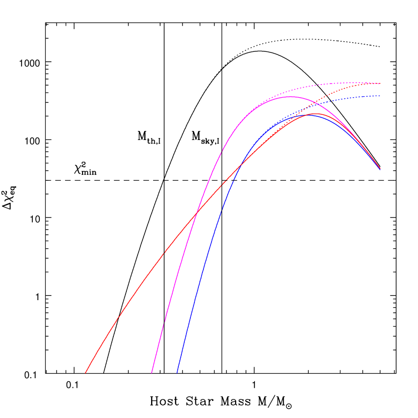
Figure 2.— $\Delta\chi^{2}_{eq}$ versus host star mass for our fiducial parameters and $r=0.1R_{\odot}$ and $P=2.5~{}{\rm days}$. The vertical lines show $M_{{th},I}$ and $M_{sky,I}$, while the horizontal dashed line shows our fiducial value for $\Delta\chi^{2}_{min}$. The dotted lines show the curves of $\Delta\chi^{2}_{eq}$ without the inclusion of the systematic error $\sigma_{sys}=0.1\%$.

We next consider the overall detection probability ${\cal P}_{tot}(M,P,r)$, and its various components, ${\cal P}_{W}$, ${\cal P}_{t}$, and ${\cal P}_{S/N}$. ${\cal P}_{t}$ is described by equations (26) and (27); ${\cal P}_{S/N}$ is described by equations (15), (16), and (17); and the window function ${\cal P}_{W}$ is shown in Figure (1). We plot these various detection probabilities, and ${\cal P}_{tot}$, versus host star mass for our set of fiducial parameter values in Figure 3a. The overall shape of the ${\cal P}_{S/N}$ curve in the top plot is simple; it shows that a transit will be detected if the star’s mass is greater than $M_{th}$. The small downturn at high masses is due to the systematic error introduced in §4.3. That is because as $M$ increases, the depth of the transit decreases (because of the increasing $R$) but the photometric precision also increases. However, by placing a limit on the measured precision, at high masses the decrease in $\delta$ is no longer offset by a decrease in $\sigma$, and so the sensitivity dips.

We combine these pieces with the mass function $dn/dM$ in Figure 3b. There are a couple interesting features of the lower plot. The mass function cuts off a little over $2M_{\odot}$ because that is the turnoff mass for a system with the fiducial parameters we are using. The probability curve for $K$ band cuts off before that point, though. That is because a detector with the fiducial values we have chosen ($D=2$m, $t_{exp}=60$s, $\theta_{pix}=0.2$ arcsec, and $N_{FW}=10^{5}$ photons) saturates at that mass in $K$, while the values for $M_{sat}$ for $I$, $V$, and $B$ are higher than $M_{to}$ for this fiducial stellar system.

Looking at the lower plot, it is clear that $I$ band is the best one to use to detect planets. The number of stars increases with decreasing mass, and it is possible to detect planets around stars of lower mass in the $I$-band. Since $N_{det}$ involves the integral of ${\cal P}_{tot}(dn/dM)$ over mass, the total number of planets detected will be larger in the $I$-band. We will see in §5.3 that the $I$ band remains optimal for most parameter combinations encountered in current transit surveys.

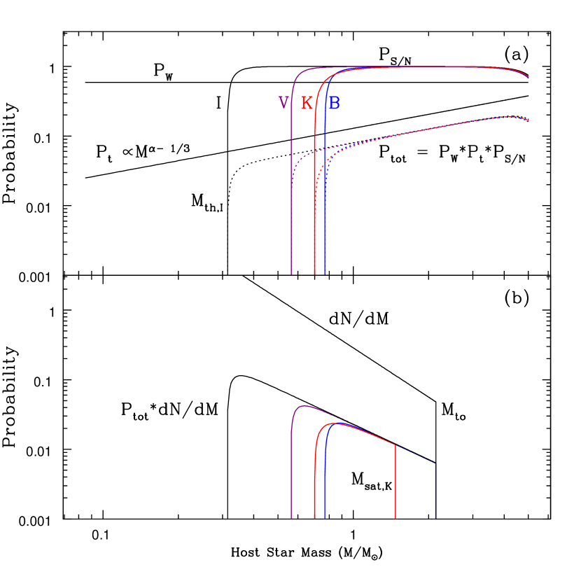
Figure 3.— Detection probabilities versus mass. Panel (a) shows ${\cal P}_{W}$, ${\cal P}_{t}$, and ${\cal P}_{S/N}$, and the product of all three, ${\cal P}_{tot}$. The curves for ${\cal P}_{tot}$ are displayed with dotted lines, to make them more easily distinguishable from the curves for ${\cal P}_{S/N}$. Panel (b) shows the mass function $dN/dM$, along with the product of it and ${\cal P}_{tot}$. In both plots, ${\cal P}_{S/N}$ and ${\cal P}_{tot}$ are shown in four different bands, $I$ (black), $V$ (purple), $B$ (blue), and $K$ (red). The plots are calculated using the fiducial parameter values in Table 1, and a period of $P=2.5$ days, for which ${\cal P}_{W}=0.63$. The cutoff in (b) is due to the fact that for a system with the fiducial parameter values used for this plot, the turnoff mass is a little over $2M_{\odot}$.

5.2. Sensitivity to Period

We next examine the sensitivity as a function of period. We consider the total detection probability ${\cal P}_{tot}$, weighted by the mass function, $dn/dM$, integrated over period, i.e. $\int{\cal P}_{tot}(dn/dM)dM$. This is shown in Figure 4.

The strong sensitivity to shorter period planets is clear, and arises from competition from several effects. The signal-to-noise probability ${\cal P}_{S/N}$ increases for increasing $P$, since a planet with a longer period will have a transit with a longer duration, and so there will be more observations during the transit and hence higher S/N. However, this effect is more than compensated by the fact that the transit probability is $\propto P^{-2/3}$, and the window probability ${\cal P}_{W}$ generally increases for smaller periods (see Figure 1), since there is a greater chance of detecting two transits for shorter periods.

5.3. Sensitivity to Parameters

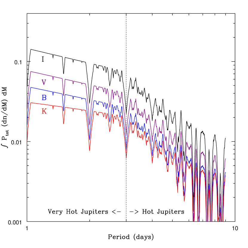
Figure 4.— The total detection probability ${\cal P}_{tot}$, weighted by the mass function $dn/dM$, and integrated over mass, i.e. $\int{\cal P}_{tot}(dn/dM)dM$, versus planet period, for our fiducial parameters (see Table 1). The window function used for this calculation is the same ${\cal P}_{W}$ as in Figure 1. The various colors represent the different observing bands, $I$ (black), $V$ (purple), $B$ (blue), and $K$ (red).

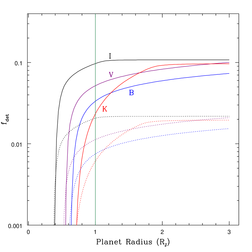
Figure 5.— The fraction of planets detected, $f_{det}$ versus planet radius, for our fiducial parameters (see Table 1). In order to convert to the number of planets detected $N_{det}$, these numbers should be multiplied by the total number of stars $N_{*}$ in the system with masses between $M=0.3M_{\odot}$ and the turn-off mass, and by the fraction $f_{p}$ of these stars with planets, i.e. $N_{det}=f_{det}f_{p}N_{*}$. The colors represent the different observing bands, $I$ (black), $V$ (purple), $B$ (blue), and $K$ (red). The solid lines show $f_{det}$ for “Very Hot Jupiters,” i.e. planets with periods $P=1-3~{}{\rm days}$. The dotted lines show $f_{det}$ for “Hot Jupiters,” planets with periods $P=3-9~{}{\rm days}$. The vertical green line indicates the fiducial value we use for the other plots, $r=0.1R_{\odot}\simeq 1R_{J}$.

In this section, we examine how the fraction of detected planets $f_{det}$ depends on the various input parameters considered and listed in Table 1. Conceptually, there are three different classes of parameters in Table 1. Five of the parameters describe the properties of the target system: $d$, $A$, $\gamma$, $\beta$, and $A_{I}$. Five of the parameters are properties of the observing setup: $D$, $t_{exp}$, $\theta_{see}$, $\Delta\chi^{2}_{min}$, and $N_{n}$. The two remaining parameters, $P$ and $r$, are properties of individual planets.

Integrating over mass, period, and radius, the fraction of planets detected is,

$$f_{det}\equiv\frac{N_{d}}{f_{p}N_{*}}=\int\int\int drdPdM\frac{d^{2}p}{drdP}{\cal P}_{tot}(M,P,R)\frac{dn}{dM}\,.$$ (40)

In Figure 5, we plot $f_{det}$ versus planet radius. We plot $f_{det}$ for the six parameters of the target system in Figure 6, and the five observing parameters in Figure 7. We shall now go though each of the parameters and describe the dependencies.

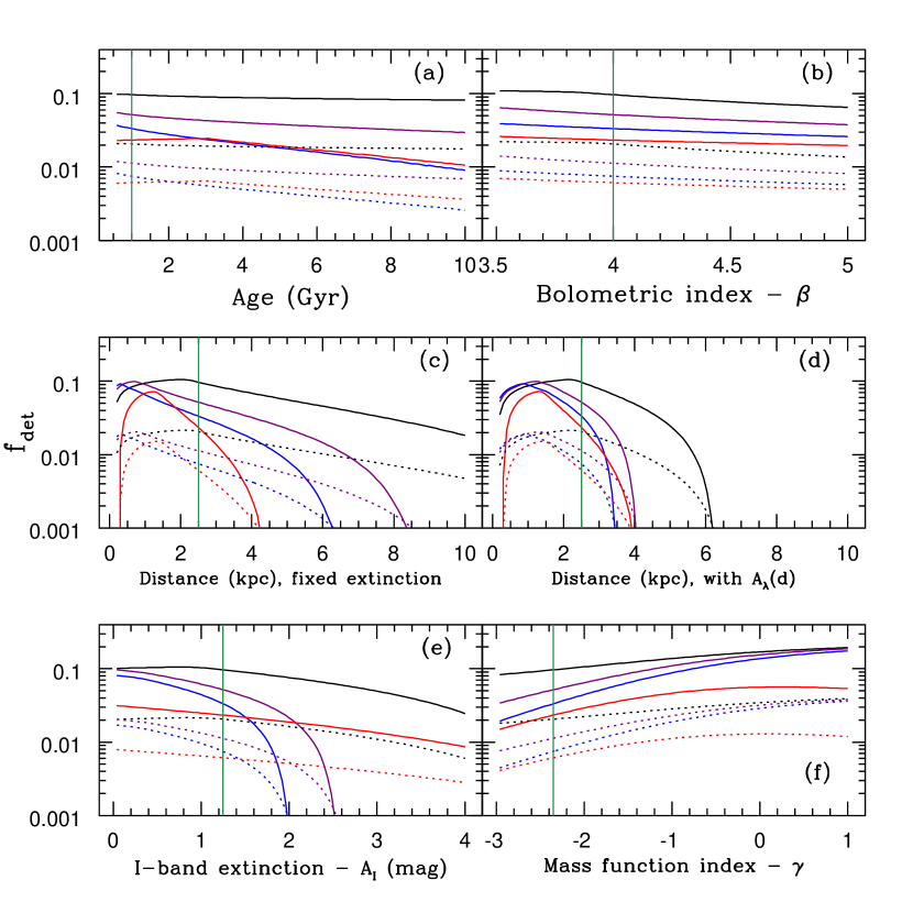
Figure 6.— The fraction of planets detected, $f_{det}$, as a function of the parameters of the target stellar system. Line types are the same as in Figure 5. The vertical green line in each plot indicates the fiducial value for that parameter used in calculating all the other plots. The panels show $f_{det}$ versus (a) age of the system, (b) power-law index of the mass-bolometric luminosity relation, (c) distance to the system, for a fixed extinction, (d) distance to the system, for a distance-dependent extinction, (e) $I$-band extinction, and (f) the index of the mass function.

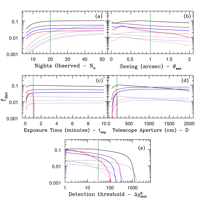
Figure 7.— Same as Fig. 6, but with $f_{det}$ as a function of the observational parameters. The panels show $f_{det}$ versus (a) number of nights of the observational campaign, (b) full-width half-maximum of the point-spread function (the seeing), (c) the exposure time, (d) the diameter of the telescope, and (e) the minimum $\chi^{2}_{min}$ required for detection.

• Radius - The dependence on planetary radius $r$ shows that detection probabilities increase very quickly up to the fiducial value of $r=0.1R_{\odot}$, at which point a transit with a planet of that radius has sufficient signal to be detected around nearly all the stars in the system. In this plot we also see that while the curves for $I$, $V$, and $B$ bands all have this similar “step-function” shape, whereas the rise for the $K$-band is more gradual.

• Age - From Figure 6a, we see $f_{det}$ is quite insensitive to the age of the system in $I$ band, and is somewhat more sensitive in the other bands. This is because, as we see in Figure 3b, a larger proportion of the planets detected in the other bands are at higher masses. The fact that $M_{sat}$ is lower than $M_{to}$ in $K$ accounts for the break in the curve in $K$.

• Bolometric Index - Figure 6b shows that $f_{det}$ is weakly dependent on the value of $\beta$. Therefore our choice of $\beta=4.0$ is not so important, as $f_{det}$ is essentially the same for $3.5<\beta<5.0$, which encompasses the whole range of values that are typically used for the mass-bolometric luminosity relation.

• Distance - This is a key parameter. A nearby system will have many saturated stars, which accounts for the turnover at small distances. For fixed extinction (Figure 6c), as the system gets further away, the signal drops and planets cannot be detected around the smaller stars in the system. For distance-dependent extinction (Figure 6d), that effect is compounded at large distances, although the extinction has much less of an effect in $K$. In both cases, for sufficiently large distances, the system transitions into the source-limited regime, at which point $f_{det}$ drops precipitously.

• Extinction - Figure 6e plots the dependence on the value of $A_{I}$, showing the effects of greater extinction at a fixed distance. In a sense, combining the effects from Figure 6c and Figure 6e gives us Figure 6d, although the combination is more complex than a simple multiplication.

• Mass Function - The slope of the mass function $\gamma$ determines the relative number of smaller stars and larger stars. The fiducial value of $\gamma=-2.35$ is the usual Salpeter slope (Salpeter, 1955). As we see in Figure 6f, the detection probabilities do not depend greatly on the exact value of the slope, although for larger values of $\gamma$ bluer bandpasses become more competitive, as expected.

• Nights Observed - In Figure 7a, we see that the an observing campaign lasting about 15 nights will detect two or more transits from nearly all the “Very Hot Jupiters” ($1~{}{\rm day}<P<3~{}{\rm days}$) that satisfy the detection threshold, but to detect two or more transits from most of the detectable “Hot Jupiters” ($3~{}{\rm days}<P<9~{}{\rm days}$), the survey should last more than twice as long. Since we assume perfect weather in this analysis, even more time should be expected to fully detect the most possible transits.

• Seeing - An increase in the seeing means an increase in the size of the PSF, and so an increase the number of pixels over which the flux of the stars is distributed. This affects $f_{det}$ is two distinct and opposite ways. First, this increases the contribution of the background noise at fixed mass, therefore increasing $M_{th}$. Second, this decreases the number of photons in the central pixel, and so increases the mass at which the detector saturates, $M_{sat}$. As discussed in §3.2, $M_{th}$ is rather weakly dependent on seeing for experiments in the background limited regime, due primarily to the fact that the mass-luminosity relation is so steep. Furthermore, the increase in $M_{th}$ is partially compensated for by the increase in $M_{sat}$. As a result, the $f_{det}$ varies very little for the typical range of seeing encountered in real observations, as seen in Figure 7b. Since the sky is so much brighter in $K$, the seeing dependence is somewhat greater in that band.

• Exposure Time - There are three effects of $t_{exp}$. First, a longer exposure time increases the total number of photons in a single observation. Second, longer exposure times decrease the number of observations per transit. These two effects effectively cancel when $t_{exp}\gg t_{read}$. The third effect of $t_{exp}$ is that very long exposure times cause bright stars to saturate. In Figure 7c the saturation effect is the reason why $f_{det}$ in $K$ falls so quickly, since for our fiducial setup the large number of sky photons alone already brings the pixels close to saturation in $K$. In the other bands complete saturation does not occur even at $t_{exp}=10$ minutes. Since saturation involves both $t_{exp}$ and $D$, we shall see in §6 that the simultaneous consideration of both factors is important.

• Telescope Aperture - This factor enters in two ways. Larger apertures allow a survey to reach the detection threshold for fainter stars, yet also lead to saturation of brighter stars. In Figure 7d in $K$ we see that $f_{det}$ plummets a little past $D=200$ cm, since at that aperture the sky photons alone saturate the pixels. In $I$, the situation is complicated. Increasing $D$ decreases $M_{th}$. However, looking back at Figure 3, we see that in $I$, $M_{th}$ is just a little larger than $0.3M_{\odot}$, which we take as the minimum observable mass. Thus increasing $D$ eventually pushes $M_{th}$ below $0.3M_{\odot}$. Any further increase in $D$ will therefore not result in additional detections at the low-mass end, and instead simply lowers $f_{det}$ as an increasing number of high-mass stars saturate the detector. In $V$ and $B$, $M_{th}$ continues to decrease for larger apertures, but due to its weak dependence on $D$, it is always above $0.3M_{\odot}$ for $D\leq 2000~{}{\rm cm}$. Further, the increase in $f_{det}$ due to decreasing $M_{th}$ is compensated for by the decrease in $M_{sat}$, such that $f_{det}$ is nearly independent of the aperture for $D\gtrsim 500~{}{\rm cm}$ and $B-$ and $V-$band observations.

• Detection threshold - The choice of $\Delta\chi^{2}_{\rm min}$ is strongly related to how much follow-up time and resources are available for confirming transit candidates. Since false positives are a big hurdle in confirming transits, it is best to choose a high value for $\Delta\chi^{2}_{min}$. As anticipated in §3.2, and seen in Figure 7e, the dependence of $f_{det}$ on $\Delta\chi^{2}_{min}$ is relatively weak until the background-limited regime is reached, at which point $f_{det}$ falls rapidly. For our fiducial parameter values which are representative of many open cluster surveys, rather stringent detection criteria of $\Delta\chi^{2}_{min}\lesssim 100$ can be tolerated without an unacceptably large reduction in the detection efficiency.

5.4. Minimum Mass

Up to this point, our results have been normalized such that $f_{det}$ is the fraction of the planets orbiting stars with masses between $0.3~{}M_{\odot}\leq M\leq M_{to}$ that are detected. We have not considered masses below $0.3~{}M_{\odot}$. The lower mass limit was chosen because this is approximately the minimum mass around which a planet was detectable in the $I$-band for our fiducial assumptions (see Fig. 2). Furthermore, it is also approximately the completeness limit of the deepest mass function determinations for rich old open clusters (e.g., Kalirai et al. 2001).

In some instances, it may be possible to detect planets around stars with masses considerably smaller than we have considered, with $M\leq 0.3M_{\odot}$. Since constraints on planets orbiting such very low mass stars are meager, we briefly consider the detectability of planets around host star masses in this regime. Specifically, we perform the same analysis, except now we consider stars with masses in the full range $M_{hb}\leq M\leq M_{to}$, where $M_{hb}=0.08~{}M_{\odot}$ is the mass at the hydrogen-burning limit. In order to make these results directly comparable to our previous results, we will continue to normalize the mass function such that $N_{*}$ is the total number of stars between $0.3~{}M_{\odot}\leq M\leq M_{to}$, and $N_{det}=f_{p}f_{det}N_{*}$, with $f_{p}$ the fraction of stars with planets, and $f_{det}$ the number of planets orbiting stars between $0.3~{}M_{\odot}\leq M\leq M_{to}$ that are detected. In this way, $f_{det}$ can now formally exceed unity, although in practice this is never the case. Figure 8b shows $f_{det}$ versus distance including stars down to the hydrogen-burning limit. We see that, for monotonically rising mass functions, it may be possible to increase the number of detections significantly by considering very low mass primaries. However, initial mass functions are observed to have breaks near $M\sim(0.3-0.5)~{}M_{\odot}$, such that this boost is probably not realized in practice, and furthermore any detections around such low-mass primaries will be quite difficult to confirm, as we discuss below. Nevertheless, the potential for constraining the planetary population of very low-mass primaries is noteworthy.

In order to determine planet masses, as well as eliminate the many kinds of astrophysical false positives that mimic planetary transits (Torres et al., 2004; Mandushev et al., 2005; Pont et al., 2005a), reasonably precise $\sim 50~{}{\rm m~{}s^{-1}}$ radial velocity (RV) follow-up measurements of candidate transits are required. Since the majority of the stars probed by transit surveys toward stellar systems are relatively faint, the ability to perform RV follow-up to this precision is a serious concern. The current state-of-the-art RV measurements on faint stars using $10{\rm m}$-class telescopes can reach precisions of $\sim 50~{}{\rm m~{}s^{-1}}$ on stars with $V\lesssim 17$ (Konacki et al., 2003b; Bouchy et al., 2005; Pont et al., 2005b). It may be possible to push this limit to somewhat fainter stars with more ambitious allocation of resources, or improvements in future technology.

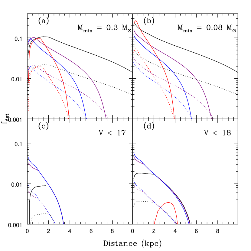
Figure 8.— Plots of $f_{det}$ versus distance. The different plots use different criteria for the minimum mass cutoff, with a fixed mass of $0.3M_{\odot}$ in Panel (a), $0.08M_{\odot}$ in Panel (b), or minimum masses corresponding to magnitude cuts $V<17$ in Panel (c) and $V<18$ in Panel (d).

In order to estimate what fraction of detected planets can be confirmed using RV follow-up, in Figure 8, we plot $f_{det}$ versus distance, where we consider only those host stars with apparent $V$-magnitudes of $V<17$ and $V<18$. These can be compared directly to the case where we consider all stars with $M\geq 0.3~{}M_{\odot}$. The first feature of Figure 8 that is noticed is that the plots of $f_{det}$ drop faster for the magnitude limited cases than for the mass limited case, because of the nature of the mass-luminosity relation. For our fiducial parameters, it is clear that the number of candidates that can be confirmed is considerably smaller than the number that can be detected. Furthermore, the advantage of observations in the $I$-band is effectively removed, since most of the additional $I$-band detections are too faint for RV confirmation.

It is clear that the ability to perform RV follow-up on candidate planetary transits must be considered carefully when designing a transit survey. The question of how to devise a photometric survey that maximizes the number of detected planets while accounting for the ability to perform spectroscopic follow-up is outside of the scope of this paper, but the formalism we have introduced here should provide the tools to do so.

6. An Application

The most obvious application of our results is to use the predictions for the number of detectable planets to choose optimal targets for a particular survey, and to derive strategies to optimize the number of detected transits for a specific target. Since the specifics of the optimal strategies will depend on detailed properties of the survey, such as the site, detector, telescope, and time allotment, here we will not attempt a comprehensive discussion, but rather simply suggest heuristic guidelines motivated by a couple of specific examples.

One important question is which targets are optimal in the sense of allowing the largest number of possible detections. There are a number of factors that may enter into target selection, including visibility, metallicity, richness, extinction, size and distance. We illustrate how our results can be used to quantify and optimize cluster selection, using the example of the trade-off between cluster distance and exposure time. As we have shown, $f_{det}$ is a strong decreasing function of cluster distance, such that closer clusters are generally preferred. However, saturation of bright stars is also more problematic for more nearby clusters. This can be partially compensated for by decreasing the exposure time, but only until $t_{exp}$ becomes comparable to $t_{read}$. In Figure 9b we show how $f_{det}$ varies with distance to the target for various exposure times. From this result, we see that clusters with distances $d\sim 2~{}{\rm kpc}$ are optimal, for telescope apertures of $D\sim 200~{}{\rm cm}$.

A somewhat different problem is to determine, given a particular target system in which one wants to search for planets, what is the optimal observational setup. If the intent of a survey is to detect all the transits of the brightest stars, then the exposure time should be set such that the survey saturates at the turnoff stars of the target system. In that case, the exposure time can be calculated using equations (10), (13), (37), and (35). On the other hand, if the intent is to configure the parameters to achieve the largest number of photometric detections, there are two factors at which we should look more closely: aperture size and exposure time. We can see in Figure 9a how $f_{det}$ varies with aperture size for various exposure times. When the aperture size is large, saturation effects reduce the detection efficiency very quickly, and this can only be partially compensated for by decreasing the exposure time. As a result, for transit surveys aiming to detect Jupiter-sized planets, telescopes with apertures of $D\sim(200-400)~{}{\rm cm}$ are optimal. Exposure times of less then a couple minutes are generally sufficient.

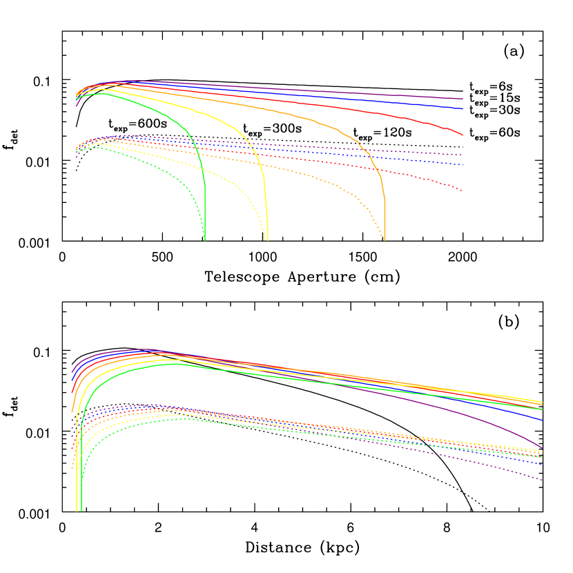
Figure 9.— The fraction of detected planets $f_{det}$ as a function of telescope aperture and distance for various exposure times, showing only the I-band curves. The solid lines represent Very Hot Jupiters ($1~{}{\rm day}<P<3~{}{\rm days}$), while the dotted lines represent Hot Jupiters ($3~{}{\rm days}<P<9~{}{\rm days}$).

These preliminary calculations provide some guide to the best places and optimal methods to look for planetary transits. Observers searching for transits can use the formalism derived here to precisely determine which systems to search for transits, and what observing setup to use.

7. Summary and Discussion

In this paper we have developed a formalism to predict the efficiency of searches for transits in stellar systems. We have taken into account most relevant parameters that affect the number of transits that can be observed, and we have described how the total number of expected transit detections depends on these parameters. Our primary results are as follows.

(1) $I$-band is optimal. For the range of parameters encountered in most transit surveys, observations in the $I$-band maximize the number of detected planetary transits. In general, redder bands are preferred also because the effects of limb-darkening are minimized, which aids in the interpretation of transit candidates and in the elimination of false positives (Mallén-Ornelas et al., 2003). However we have not taken into account the variation in quantum efficiency of detectors as a function of wavelength. This is likely a small effect. For some detectors, fringing can be a serious problem in the $I$-band. Thus, in some cases, somewhat bluer bands (i.e. the $R$-band) may be preferable. Surprisingly, in essentially no case do we find that observations in the $K$-band outperform those in the $I$-band.

(2) The ${\rm S/N}$ depends weakly on primary mass. For the $I$-band, and assuming only Poisson uncertainties, the signal-to-noise ratio of a planetary transit is an extremely weak function of mass for sources with flux above that of the sky background. For sources with flux below sky, the ${\rm S/N}$ is a very strong decreasing function of mass.

(3) The number of detections is proportional to the number of stars above sky. As a direct consequence of item (2), if one can find planets around any stars in the target system, one can detect planets around all stars in the system with fluxes above sky. Therefore, the number of planets that are detectable is proportional to the number of stars with flux above sky. This is quite distinct from the usual assumption that the number of detectable planets is proportional to the number of stars with photometric error less than a given precision, usually taken to be $\sim 1\%$. Estimates based on this canonical criteria will typically be incorrect.

(4) Most planets will be detected around stars with flux near sky. Under the typically valid assumption of a mass function that rises toward lower-mass stars, item (3) implies that most planets will be detected around stars that have fluxes approximately equal to the flux of the sky background.

(5) Planets orbiting stars near sky must be detectable. The primary requirement for a successful transit survey is that the planets orbiting stars with fluxes near the sky background must be detectable. This requirement is formulated mathematically in equation (19). Provided this requirement is met, the number of detected planets is a rather weak function of the radius of the planet, index of the bolometric mass-luminosity relation, age of the system, index of the mass function, seeing, exposure time, telescope aperture, and the detection threshold.

(6) The richest, closest systems are optimal. The number of detected planets has the strongest dependence on the distance modulus, the distance and extinction to the cluster. Systems at distances of $d\lesssim 2~{}{\rm kpc}$ are optimal. Very nearby ($d\lesssim 1~{}{\rm kpc}$) systems may have difficulties with saturation of bright stars, as well fitting within the field-of-view of the detector.

(7) Follow-up of the majority of candidates may be difficult. The majority of planets in typical target systems are likely to be detected around stars with apparent magnitudes of $V\gtrsim 17$, making precision RV follow-up difficult. This is an important conclusion which may affect the design of transit surveys. Difficulties with RV follow-up are partially ameliorated by the fact that surveys toward stellar systems are much less prone to the ambiguities with the interpretation of candidate detections encountered in field surveys, since the properties of the primaries are better known.

There are a number of ways in which our analysis could be expanded and refined. For instance, we do not take into account the metallicity of the observed systems. Studies have indicated that planets are more common around high-metallicity stars (Fischer & Valenti, 2005), and as that correlation becomes better characterized we can add metallicity to the parameters we examine. It would also be useful to include the effects of observability on the window function, which is important for the selection of optimal targets. Our analysis also does not account for bad weather. Further work could examine what kinds of inclement weather are most damaging for a transit search and could possibly address the question of whether it is possible to partially compensate for inclement weather by adopting more sophisticated observing strategies. Another potential refinement would be to account for different forms for the mass function, rather than relying on the simple Salpeter shape we use in this paper, such as a broken power-law function with different power-law indices for high mass and low mass stars. Lastly, we do not account for stellar binarity, which also generally decreases detection probability.

Appendix A Total S/N Formulation

In the main text, we derived expressions for the signal-to-noise ratio of a transiting planet ${\rm S/N}=(\Delta\chi^{2})^{1/2}$ for a single transit. The probability ${\cal P}_{S/N}$ that a planet will have a ${\rm S/N}$ that exceeds a given threshold, and all subsequent calculations, were based on this single-transit ${\rm S/N}$ criterion. However, planets will generally exhibit multiple transits, and it is possible, by folding an observed light curve about the proper period, to improve the total ${\rm S/N}$ over that of a single transit by $\sim n^{1/2}$, where $n$ is the number of observed transits. In fact, popular transit search algorithms operate on phase-folded light curves, and so trigger based on this total signal-to-noise ratio (Kovács et al., 2002; Aigrain & Irwin, 2004; Weldrake & Sackett, 2005). It is therefore interesting to rederive our expressions based on this total ${\rm S/N}$ formulation.

The general expression for the number of detected planets $N_{det}$ remains the same, but the expression for the total detection probability ${\cal P}_{tot}(M,P,r)$ needs to be altered,

$${\cal P}_{tot}(M,P,r)={\cal P}_{t}(M,P){\cal P}_{S/N}^{tot}(M,P,r){\cal P}_{W}(P),$$ (A1)

where ${\cal P}_{t}$ and ${\cal P}_{W}$ are the transit and window probabilities as before, and ${\cal P}_{S/N}^{tot}$ is now the probability that the total signal-to-noise ratio is higher than some threshold value.

The total signal-to-noise probability, ${\cal P}_{S/N}^{tot}$ can be derived in an analogous way as the one-transit signal-to-noise probability (see §2.2.3). We begin by defining $d{\cal P}_{S/N}^{tot}/db\equiv\Theta\left[\Delta\chi^{2}_{tr}-\Delta\chi_{min}^{2}\right]$, where $\Delta\chi^{2}_{tr}$ is the difference in $\chi^{2}$ between a constant flux and transit fit to the data,

$$\Delta\chi^{2}_{tr}=N_{tr}^{tot}\left(\frac{\delta}{\sigma}\right)^{2}.$$ (A2)

Here $N_{tr}^{tot}$ is the total number of observations taken during any transit, and $\delta$ and $\sigma$ are as before.

For no aliasing, and periods much shorter than the length of the observational campaign, the total number of observations during transit is simply the transit duty cycle $t_{tr}/P$, times the total number of observations $N_{tot}$,

$$N_{tr}^{tot}=\frac{t_{tr}}{P}N_{tot}.$$ (A3)

In fact, for campaigns of finite durations from single sites, aliasing cannot be ignored, and there will be a dispersion in the fraction of points during transit about the naive estimate $t_{tr}/P$. For long campaigns lasting more than $\sim 40~{}{\rm days}$, aliasing effects are generally not dominant, although they are still significant (see Gaudi et al. 2004 for examples). They can be accounted for by integrating $d^{2}{\cal P}_{S/N}/d\phi db$ over the transit phase $\phi$ as well as impact parameter $b$. For simplicity, we will ignore aliasing effects here, and assume equation (A3).

Since $t_{tr}=\sqrt{1-b^{2}}t_{eq}$, we can write,

$$\Delta\chi^{2}_{tr}=\Delta\chi^{2}_{eq}\sqrt{1-b^{2}},\qquad\Delta\chi^{2}_{eq}=N_{tot}\frac{t_{eq}}{P}\left(\frac{\delta}{\sigma}\right)^{2},.$$ (A4)

The total signal-to-noise probability is then just the integral over impact parameter,

$${\cal P}_{S/N}^{tot}=\int_{0}^{1}\frac{d{\cal P}_{S/N}}{db}db,$$ (A5)

which yields

$${\cal P}_{S/N}^{tot}=\sqrt{1-\left(\frac{\Delta\chi^{2}_{min}}{\Delta\chi^{2}_{eq}}\right)^{2}}\,,$$ (A6)

if $\Delta\chi^{2}_{min}\leq\Delta\chi^{2}_{eq}$, and ${\cal P}_{S/N}=0$ otherwise.

We can write $\chi^{2}_{eq}$ in more explicit terms using the expressions for $\sigma$, $\delta$, and $t_{eq}$ derived previously. The additional new ingredient is the expression for $N_{tot}$. If we assume that the campaign lasts $N_{n}$ nights, each with a duration of $t_{night}$, and that observations are made continuously, then the total number of data points is

$$N_{tot}=\frac{t_{night}}{t_{exp}+t_{read}}N_{n}.$$ (A7)

Combining this with the expressions we derived in §2.2.3, we arrive at the expression,

$$\Delta\chi^{2}_{eq}=(1024\pi)^{-1/3}\frac{t_{exp}}{t_{read}+t_{exp}}\left(\frac{r}{R}\right)^{4}\left(\frac{D}{d}\right)^{2}\left(\frac{R^{3}}{GMP^{2}}\right)^{1/3}t_{night}N_{n}L_{\lambda}10^{-0.4A_{\lambda}}$$

$$\times\left(1+\frac{S_{sky,\lambda}\Omega 4\pi d^{2}}{L_{\lambda}10^{-0.4A_{\lambda}}}\right)^{-1},$$ (A8)

which can be compared to the analogous expression for a single transit, equation (12). Comparison of equation (12) and equation (A8) reveals that the ratio of $\chi^{2}_{eq}$ for the total signal-to-noise ratio formulation to $\chi^{2}_{eq}$ for the single-transit formulation is $\propto P^{-1}$. Thus the total S/N formulation favors short-period planets more heavily than the single-transit formulation.

Appendix B Effect of Partial Transits

Let us return for the moment to our definition of $N_{tr}$. This variable represents the number of observations of the system during a single transit. We stated earlier that $N_{tr}=t_{tr}/(t_{read}+t_{exp})$. However, that formula is only valid if the entire transit is observed during the night; it does not hold if only partial transits are observed, i.e. if the transit begins before the start of the night or ends after the end of the night. In those cases the transit is observed for a time less than $t_{tr}$, the number of observations during transit is less than $N_{tr}$, and therefore the signal-to-noise is less than the naive estimate in §2.2.3.

To account for partial transits, we rewrite the transit duration as,

$$t_{tr}=t_{eq}\sqrt{1-b^{2}}f(\phi),$$ (B1)

where $f(\phi)$ is the fraction of the total transit duration that occurs during the observation window, as a function of the phase $\phi$ of the transit. For uniform sampling, and $t_{eq}\leq t_{night}$, this is simply,

$$f(\phi)=\left\{\begin{array}[]{ll}\frac{1}{2}+\phi\frac{t_{night}}{t_{eq}\sqrt{1-b^{2}}}&{\rm if}\qquad 0\leq\phi\leq\frac{1}{2}\frac{t_{eq}\sqrt{1-b^{2}}}{t_{night}}\\ 1&{\rm if}\qquad|\phi-\frac{1}{2}|\geq\frac{1}{2}\frac{t_{eq}\sqrt{1-b^{2}}}{t_{night}}-\frac{1}{2}\\ \frac{1}{2}+\frac{t_{night}}{t_{eq}\sqrt{1-b^{2}}}(1-\phi)&{\rm if}\qquad\phi\geq 1-\frac{1}{2}\frac{t_{eq}\sqrt{1-b^{2}}}{t_{night}}\geq 1\\ 0&{\rm otherwise}\end{array}\right.,$$ (B2)

where $\phi=0$ is the beginning of the night and $\phi=1$ is the end of the night. Note also that we have also conservatively assumed that a transit cannot be detected if it is observed for less than half of its total duration.

Following the discussion in §2.2.3, we write

$$\frac{d^{2}{\cal P}_{S/N}}{dbd\phi}=\Theta\left[\Delta\chi_{eq}^{2}\sqrt{1-b^{2}}f(\phi)-\Delta\chi_{min}^{2}\right].$$ (B3)

Proceeding in the same way as in §2.2.3, we integrate equation (B3) over $b$ from 0 to $b_{max}$, and $\phi$ from 0 to 1, assuming a uniform distribution for $b$ and $\phi$, solve for $b_{max}$, i.e.,

$${\cal P}_{S/N}=\int_{0}^{1}db\int_{0}^{1}d\phi\frac{d{\cal P}_{S/N}}{dbd\phi}.$$ (B4)

We do not attempt to solve equation (B4) analytically, rather we evaluate it numerically, noting that ${\cal P}_{S/N}$ depends only on the ratios $\Delta\chi^{2}_{min}/\chi^{2}_{eq}$ and $t_{eq}/t_{night}$. Figure 10 shows ${\cal P}_{S/N}$ as a function of $\Delta\chi^{2}_{min}/\chi^{2}_{eq}$ for equatorial transit durations lasting $10-50\%$ of the night. We also show the result for the simplified assumption of $t_{eq}\ll t_{night}$ that we adopted throughout. We conclude that our simple assumption is sufficient for purposes, but note that it overestimates ${\cal P}_{S/N}$ by as much as $25\%$ for certain combinations of parameters.

Figure 10.— The probability ${\cal P}_{S/N}$ that a planet, producing $\Delta\chi^{2}=\Delta\chi^{2}_{eq}$ for an equatorial transit, will yield a $\Delta\chi^{2}$ greater than a given threshold $\Delta\chi^{2}_{min}$, when integrated over all impact parameters and phases, for various values of the ratio of the equatorial transit duration $t_{eq}$ to the duration of the night $t_{night}$. The solid line shows the approximation ${\cal P}_{S/N}=\sqrt{1-(\Delta\chi^{2}_{min}/\Delta\chi^{2}_{eq})^{2}}$ used in the main test, which is valid for $t_{eq}\ll t_{night}$

References

- Aigrain & Irwin (2004) Aigrain, S., & Irwin, M. 2004, MNRAS, 350, 331
- Alonso et al. (2004) Alonso, R., et al. 2004, ApJ, 613, L153
- Bakos et al. (2004) Bakos, G., Noyes, R. W., Kovács, G., Stanek, K. Z., Sasselov, D. D., & Domsa, I. 2004, PASP, 116, 266
- Binney & Merrifield (1998) Binney, J. & Merrifield, M. 1998, Galactic Astronomy (Princeton: Princeton University Press)
- Bessell et al. (1998) Bessell, M. S., Castelli, F., & Pletz, B. 1998, A&A, 333, 231B
- Borucki, et al. (2001) Borucki, W. J., Caldwell, D., Koch, D. G., Webster, L. D., Jenkins, J. M., Ninkov, Z., & Showen, R. 2001, PASP, 113, 439B
- Bouchy et al. (2004) Bouchy, F., Pont, F., Santos, N. C., Melo, C., Mayor, M., Queloz, D., & Udry, S. 2004, A&A, 421, L13
- Bouchy et al. (2005) Bouchy, F., Pont, F., Melo, C., Santos, N. C., Mayor, M., Queloz, D., & Udry, S. 2005, A&A, 431, 1105
- Burke et al. (2003) Burke, C. J., DePoy, D. L., Gaudi, B. S., Marshall, J. L., Pogge, R. W. 2003, ASP Conf. Ser. 294: Scientific Frontiers in Research on Extrasolar Planets, 379B
- Burke et al. (2005) Burke, C. J., Gaudi, B. S., DePoy, D. L., & Pogge, R. W. 2005, in preparation
- Bramich et al. (2005) Bramich, D. M., et al. 2005, MNRAS, 359, 1096B
- Bruntt et al. (2003) Bruntt, H., Grundahl, F., Tingley, B., Frandsen, S., Stetson, P. B., & Thomsen, B. 2003, A&A, 410, 323
- Charbonneau et al. (2002) Charbonneau, D., Brown, T. M., Noyes, R. W., & Gilliland, R. L. 2002, ApJ568, 377C
- Charbonneau et al. (2005) Charbonneau, D., et al. 2005, ApJ, in press (astro-ph/0503457)
- Deeg et al. (2004) Deeg, H. J., Alonso, R., Belmonte, J. A., Alsubai, K., Horne, K., & Doyle, L. 2004, PASP, 116, 985
- Deming et al. (2005) Deming, D., Seager, S., Richardson, L. J., & Harrington, J. 2005, Nature, 434, 740
- Dorsher et al. (2005) Dorsher, S., Gould, A., & Gaudi, B.S. 2005, in preparation
- Drake & Cook (2004) Drake, A. J., & Cook, K. H. 2004, ApJ, 604, 379
- Dreizler et al. (2002) Dreizler, S., Rauch, T., Hauschildt, P., Schuh, S. L., Kley, W., & Werner, K. 2002, A&A, 391, L17
- Fischer & Valenti (2005) Fischer, D. A., & Valenti, J. 2005, ApJ, 622, 1102
- Gallardo et al. (2005) Gallardo, J., Minniti, D., Valls-Gabaud, D., & Rejkuba, M. 2005, A&A, 431, 707
- Gaudi (2000) Gaudi, B. S. 2000, ApJ, 539, L59
- Gaudi et al. (2004) Gaudi, B. S., Seager, S., & Mallen-Ornelas, G. 2005, ApJ, 623, 472
- Gaudi (2005) Gaudi, B. S. 2005, ApJ, submitted (astro-ph/0504123)
- Gilliland et al. (2000) Gilliland, R. L., et al. 2000, ApJ, 545, L47
- Hidas et al. (2005) Hidas, M. G., et al. 2005, MNRAS, submitted (astro-ph/0501269)
- Horne (2003) Horne, K. 2003, ASP Conf. Ser. 294: Scientific Frontiers in Research on Extrasolar Planets, 294, 361
- Janes (1996) Janes, K. 1996, J. Geophys. Res., 101, 14853
- Kalirai et al. (2001) Kalirai, J. S., Ventura, P., Richer, H. B., Fahlman, G. G., Durrell, P. R., D’Antona, F., & Marconi, G. 2001, AJ, 122, 3239
- Kane et al. (2004) Kane, S. R., Collier Cameron, A., Horne, K., James, D., Lister, T. A., Pollacco, D. L., Street, R. A., & Tsapras, Y. 2004, MNRAS, 353, 689
- Konacki et al. (2003a) Konacki, M., Torres, G., Jha, S., & Sasselov, D. D. 2003a, Nature, 421, 507
- Konacki et al. (2003b) Konacki, M., Torres, G., Sasselov, D. D., & Jha, S. 2003b, ApJ, 597, 1076
- Konacki et al. (2004) Konacki, M., et al. 2004, ApJ, 609, L37
- Konacki et al. (2005) Konacki, M., et al. 2005, ApJ, 624, 372
- Kovács et al. (2002) Kovács, G., Zucker, S., & Mazeh, T. 2002, A&A, 391, 369
- Lejeune, Cuisinier, & Buser (1998) Lejeune, T., Cuisinier, F., & Buser R. 1998, A&AS 130, 65
- Mallén-Ornelas et al. (2003) Mallén-Ornelas, G., Seager, S., Yee, H. K. C., Minniti, D., Gladders, M. D., Mallén-Fullerton, G. M., & Brown, T. M. 2003, ApJ, 582, 1123
- Mandushev et al. (2005) Mandushev, G., et al. 2005, ApJ, 621, 1061
- McCullough et al. (2004) McCullough, P. R., Stys, J., Valenti, J., Fleming, S., Janes, K., & Heasly, J. 2004, BAAS205, 135.12
- Mochejska et al. (2005) Mochejska, B. J., et al. 2005, AJ, 129, 2856
- Pont et al. (2004) Pont, F., Bouchy, F., Queloz, D., Santos, N., Melo, C., Mayor, M., & Udry, S. 2004, A&A, 426, L15
- Pont et al. (2005a) Pont, F., Melo, C. H. F., Bouchy, F., Udry, S., Queloz, D., Mayor, M., & Santos, N. C. 2005a, A&A, 433, L21
- Pont et al. (2005b) Pont, F., Bouchy, F., Melo, C., Santos, N. C., Mayor, M., Queloz, D., & Udry, S. 2005b, A&A, submitted (astro-ph/0501615)
- Pepper et al. (2004) Pepper, J., Gould, A., & DePoy, D. L. 2004, in AIP Conf. Proc. 713, The Search for Other Worlds, 185
- Popper (1980) Popper, D. M. 1980 ARA&A, 18, 115P
- Salpeter (1955) Salpeter, E. E. 1955, ApJ, 121, 161
- Street et al. (2003) Street, R. A., et al. 2003, MNRAS, 340, 1287
- Torres et al. (2004) Torres, G., Konacki, M., Sasselov, D. D., & Jha, S. 2004, ApJ, 614, 979
- Udalski et al. (2002a) Udalski, A., et al. 2002a, AcA, 52, 1
- Udalski et al. (2002b) Udalski, A., Zebrun, K., Szymanski, M., Kubiak, M., Soszynski, I., Szewczyk, O., Wyrzykowski, L., & Pietrzynski, G. 2002a, AcA, 52, 115
- Udalski et al. (2002c) Udalski, A., Szewczyk, O., Zebrun, K., Pietrzynski, G., Szymanski, M., Kubiak, M., Soszynski, I., & Wyrzykowski, L. 2002c, AcA, 52, 317
- Udalski et al. (2003) Udalski, A., Pietrzynski, G., Szymanski, M., Kubiak, M., Zebrun, K., Soszynski, I., Szewczyk, O., & Wyrzykowski, L. 2003, AcA, 53, 133
- Udalski et al. (2004) Udalski, A., Szymanski, M. K., Kubiak, M., Pietrzynski, G., Soszynski, I., Zebrun, K., Szewczyk, O., & Wyrzykowski, L. 2004, AcA, 54, 313
- Tabachnik & Tremaine (2002) Tabachnik, S. & Tremaine, S. 2002, MNRAS, 335, 151
- Vidal-Madjar et al. (2003) Vidal-Madjar, A., Lecavelier des Etangs, A., Désert, J.-M., Ballester, G. E., Ferlet, R., Hébrard, G., & Mayor, M. 2003, Nature, 422, 143
- Vidal-Madjar et al. (2004) Vidal-Madjar, A., et al. 2004, ApJ, 604, L69
- von Braun et al. (2005) von Braun, K., Lee, B. L., Seager, S., Yee, H. K. C., Mallen-Ornelas, G., & Gladders., M. D. 2005, PASP, 117, 141
- Weldrake & Sackett (2005) Weldrake, D. T. F., & Sackett, P. D. 2005, ApJ, 620, 1033
- Weldrake et al. (2005) Weldrake, D. T. F., Sackett, P. D., Bridges, T. J., & Freeman, K. C. 2005, ApJ, 620, 1043
- Yi et al. (2001) Yi., S., Demarque, P., Kim, Y. C., Lee, Y. W., Ree, C. H., Lejune, T., & Barnes, S. 2001, ApJS136, 417