Restframe $I$-band Hubble diagram for type Ia supernovae up to redshift $z\sim$ 0.5

We present a novel technique for fitting restframe $I$-band light curves on a data set of 42 Type Ia supernovae (SNe Ia). Using the result of the fit, we construct a Hubble diagram with 26 SNe from the subset at $0.01<z<0.1$. Adding two SNe at $z\sim 0.5$ yields results consistent with a flat $\Lambda$-dominated “concordance universe” ($\Omega_{M},\Omega_{\Lambda}$)=(0.25,0.75). For one of these, SN 2000fr, new near infrared data are presented. The high redshift supernova NIR data are also used to test for systematic effects in the use of SNe Ia as distance estimators. A flat, $\Lambda=0$, universe where the faintness of supernovae at $z\sim 0.5$ is due to grey dust homogeneously distributed in the intergalactic medium is disfavoured based on the high-z Hubble diagram using this small data-set. However, the uncertainties are large and no firm conclusion may be drawn. We explore the possibility of setting limits on intergalactic dust based on $B-I$ and $B-V$ colour measurements, and conclude that about 20 well measured SNe are needed to give statistically significant results. We also show that the high redshift restframe $I$-band data points are better fit by light curve templates that show a prominent second peak, suggesting that they are not intrinsically underluminous.

1 Introduction

Observations of Type Ia supernovae in the restframe $B$-band at redshifts of $z\sim 0.5$ and above have shown that they are best fit by a cosmological model that includes a cosmological constant or some other form of dark energy (Perlmutter et al., 1998; Garnavich et al., 1998; Riess et al., 1998; Schmidt et al., 1998; Perlmutter et al., 1999; Tonry et al., 2003; Knop et al., 2003; Riess et al., 2004). The evidence for dark energy is supported by cross-cutting cosmological results, such as the measurement of the cosmic microwave background anisotropy, which indicates a flat universe (De Bernardis et al., 2000; Jaffe et al., 2001; Sievers et al., 2003; Spergel et al., 2003); the evolution in the number density of X-ray emitting galaxy clusters (Borgani et al., 2001; Henry, 2001; Schuecker et al., 2003) and galaxy redshift surveys (Efstathiou et al., 2002), which indicate that $\Omega_{\rm M}\approx 0.3$. Taken together, these independent measurements suggest a concordance universe with ($\Omega_{\rm M}$,$\Omega_{\Lambda}$)$\cong$(0.25,0.75). However, the SN Ia Hubble diagram remains the most direct approach currently in use for studying cosmic acceleration, and, thus, possible systematic effects affecting the observed brightness of Type Ia supernovae should be carefully considered, such as uncorrected host galaxy extinction (see e.g. Rowan-Robinson (2002)), dimming by photon-axion mixing over cosmological distances (Csaki et al., 2002; Deffayet et al., 2001; Mörtsell et al., 2002; Östman & Mörtsell, 2004) and extinction by intergalactic grey dust (Aguirre, 1999a, b; Mörtsell & Goobar, 2003). Some of these have already been addressed in previous SCP publications, see e.g. Perlmutter et al. (1997, 1998); Sullivan et al. (2003); Knop et al. (2003).

Determining cosmological distances through Type Ia supernova fluxes at longer restframe wavelengths offers potential advantages, e.g. less extinction by dust along the line of sight, either in the host galaxy or in the intergalactic medium. On the other hand, the “standard candle” properties at these wavelengths and the possibility of additional systematic effects need to be investigated.

In the restframe $I$-band, the uncertainties in extinction corrections are significantly smaller than those in the $B$-band. For example, for Milky-Way type dust ($R_{V}\sim 3$) the ratio of extinction for the two bands is sizable, $A_{B}/A_{I}\sim 2-3$. In general, the extinction corrections become less dependent on our knowledge of intrinsic supernova colours and dust properties.

SNe Ia $I$-band light curves typically show a second peak 15-30 days after the first maximum. It has been suggested that the intensity and time-difference between the first and second $I$-band peaks are related to the intrinsic luminosity of the Type Ia SNe, appearing later and more evident for normal Type Ia and earlier and fainter for underluminous ones (Hamuy et al., 1996a; Wang et al., 2005). Thus, building $I$-band light curves for Type Ia supernovae offers the possibility of probing brightness evolution.

The scope of this work is to test the feasibility of using the restframe $I$-band for cosmological distance measurements, using data available to date, and to assess the importance of observing in this wavelength range for future samples of SNe. For that purpose, we develop a template fitting technique, which we apply to 42 nearby SNe Ia, to estimate the first ($I_{\rm max}$) and second ($I_{\rm sec}$) $I$-band light curve peaks. We use the fitted $I_{\rm max}$ of 26 of these SNe Ia, which are in the Hubble flow, together with two high redshift SNe Ia: SN 2000fr, at redshift $z=0.543$, for which new infrared data are presented, and SN 1999ff, at $z=0.455$, available in literature (Tonry et al., 2003), to build a Hubble diagram reaching out to $z\sim 0.5$.

The properties of the second peak in the restframe $I$-band light curves are investigated. Furthermore, additional colour information is used to test for extinction by non-conventional dust for the $z\sim 0.5$ supernovae. In a related work, Riess et al. (2000) used $B-I$ colours of SN 1999Q, in the same redshift range. This SN, however, is not included in our analysis, since we find inconsistencies with the published data (see Section 4.3).

2 I-band light curve fitting

The second light curve peak seen in $I$-band for nearby Type Ia SNe varies in strength and position with respect to the primary maximum. This complicates the use of a singly parametrised $I$-band template, such as those currently applied in the $B$- and $V$-band, (see e.g. Perlmutter et al. (1997); Goldhaber et al. (2001) for an example of the timescale stretch factor approach), for light curve fitting.

Contardo et al. (2000) proposed a model composed of as many as 4 functions for a total of 10 parameters in order to fit all $UBVRI$-bands. Their method used two Gaussian functions to fit the two peaks, together with a straight line to fit the late time decline and an exponential factor for the pre-max rising part of the light curve. In this way, it is possible to describe Type Ia SNe light curves over a wide range of epochs and in all optical bands, though, as the authors recognise, it does not represent accurately the second peak in the $I$-band due to the influence of the linear decline. However, the main disadvantage of their method, for our purpose, is the large number of free parameters, which requires very well sampled light curves.

We have therefore developed a method for fitting $I$-band light curves using five free parameters and one template used twice to describe the two peaks. As our goal is only to measure the position and amplitude of the two peaks, we limit the fit to 40 days after maximum, neglecting the late time decline. Our fitting procedure can be summarised as follows: one template is used to fit the time ($t_{1}$) and the first peak magnitude ($I_{1}$), together with a stretch factor ($s_{I}$), which is also applied to the second template shifted in time to fit the time ($t_{2}$) and magnitude of the second peak ($I_{2}$). The underlying function is

$$I=I_{1}{\cal T}(s_{I}(t-t_{1}))+I_{2}{\cal T}(s_{I}(t-t_{2}))$$

where ${\cal T}$ is the template. The five parameters fitted are thus: $\{t_{1},t_{2},I_{1},I_{2},s_{I}\}$, (see Table 1). A similar approach is also proposed by Wang et al. (2005) who call it “super-stretch” to emphasise its extension of the stretch approach.

The use of this function in place of the one described by Contardo et al. (2000), reduces the number of free parameters by a factor of two. Implicitly, we have thus assumed that the rising part of the $I$-band is the same as in the template used, i.e. the $B$-band. As we will see, this assumption is not always true. Note that, unless otherwise specified, the supernova phase always refers to the time relative to restframe $B$-band light curve maximum.

$t_{1}$	time of the peak of the first ${\cal T}$ template
$I_{1}$	peak magnitude of the first ${\cal T}$ template
$t_{2}$	time of the peak of the second ${\cal T}$ template
$I_{2}$	peak magnitude of the second ${\cal T}$ template
$s_{I}$	stretch factor of the time axis
$t_{\rm max}$	time of the first $I$ light curve peak
$I_{\rm max}$	first $I$ light curve peak magnitude
$t_{\rm sec}$	time of the second $I$ light curve peak
$I_{\rm sec}$	second $I$ light curve peak magnitude

Table 1: Summary of the parameters used in this work to describe the $I$-band light curve. The first five parameters are determined by fitting the data (see text for details). The next four parameters are determined from the first set and are the actual time and peak values of the light curve.

2.1 The low-redshift data set

We applied this method to fit a sample of local SNe Ia for which both $B$ and $I$-band data are available in the literature. The SNe primarily come from the Calan/Tololo (Hamuy et al., 1996a), CfA (Riess et al., 1999) and CfA2 (Jha, 2002) data sets. Data from three other well studied individual supernovae were also included: SN 1989B (Wells et al., 1994), SN 1994D (Richmond et al., 1995) and the underluminous supernova SN 1991bg. We have used two data sets in restframe $I$-band for SN 1991bg, one published by Filippenko et al. (1992b) with quite good coverage from about 3 days after $B$-band maximum light to +60 days, and another published by Leibundgut et al. (1993) with four data points, the first of which is at the time of $B$-band maximum. The agreement between the two data sets was assessed by comparing the measurements taken at the same date, i.e. JD=2448607, where we found a difference of 0.06 mag. We take this as an estimate of the measurement uncertainty in data of Leibundgut et al. (1993) as no uncertainties are reported in that work.

2.2 Fitting method and results

Only supernovae with at least 6 $I$-band data points and time coverage constraining both peaks were selected for light curve fitting. This resulted in a total of 42 SNe. Table 2 lists the parameters resulting from the fitting procedure. Since the dominant uncertainties are symmetric in units of flux, we performed the fit in flux rather than magnitudes. The parameters given in Table 2 are transformed into magnitudes.

Prior to fitting, all data points were $k$-corrected to restframe $I$-band as in Kim et al. (1996) and Nugent et al. (2002), assuming a Bessell $I$-band filter transmission curve (Bessell, 1990) and time information from the available $B$-band data. A new spectroscopic template, which is a slightly modified version of the template found in Nugent et al. (2002), was built for computing the $k$-corrections. We have preserved the SED from the UV through the Si II 6150Å feature, following Nobili et al. (2003), but red ward of that we have incorporated additional spectra from the Supernova Cosmology Project (SCP) Spring 1999 search (Aldering, 2000; Nugent & Aldering, 2000) to improve this region as the original template was sparse and required a lot of interpolation. A potential source of systematic uncertainty in the $k$-corrections is due to the wide Ca IR triplet absorption feature, found to vary considerably among Type  Ia supernovae (Strolger et al., 2002; Nugent et al., 2002). We have estimated this systematic uncertainty as a function of redshift for $0.01<z<0.1$ by computing the $k$-correction for diverse nearby SNe Ia at different epochs. The dispersion in the $k$-correction increases with redshift, reaching 0.05 mag. at $z=0.1$. We take this as a conservative estimate of the uncertainty in all $k$-corrections in this wavelength region.

Note that the values of $I_{2}$ reported in Table 2 are not the actual magnitudes of the secondary peak , $I_{\rm sec}$, but a parameter indicating the size of the contribution of the second template to the overall I-band light curve.

In Fig. 1, all the fitted light curves are shown. They are sorted in chronological order, except for the two very underluminous supernovae: SN 1991bg and SN 1997cn, displayed at the bottom of the figure. As the date of the $B$-band maximum for SN 1997cn is unknown, the origin of the time axis was set to the epoch ($JD=2450597.75$) when this supernova was first observed. Note that the second peak of underluminous supernovae is almost completely absent, resulting in a value of $I_{2}$ $\sim$ 2.5 to 3 magnitudes fainter than $I_{1}$.

Our sample includes SNe that are classified as spectroscopically peculiar, showing similarities with the over-luminous SN 1991T (Filippenko et al., 1992a; Ruiz-Lapuente et al., 1992; Phillips et al., 1992). These are SN 1995bd, SN 1997br, SN 1998ab, SN 1998es, SN 1999aa, SN 1999ac, SN 1999dq and SN 1999gp (Li et al., 2001; Howell, 2001; Garavini et al., 2004). One supernova, SN 1993H, was reported to show similarities with the spectrum of the peculiar underluminous SN 1986G (Hamuy et al., 1993). However, as we will see in this work, we do not find all of these to show peculiarities in their $I$-band light curve shape when compared to spectroscopically normal SNe Ia. Recently, Krisciunas et al. (2003), built the Hubble diagram for SNe Ia in infrared $J,H$ and $K$-bands out to $z=0.04$, and reported that three spectroscopically peculiar SNe, SN 1999aa, SN 1999ac and SN 1999aw, do not show a behaviour different than that of normal SNe. With the aim to assess a greater homogeneity of SNe as standard candles in the $I$-band than in $B$-band, we choose not to exclude peculiar SNe from our sample, and instead monitor possible deviant behaviour of these objects.

Analysing the results of our fits, we found that Type Ia SNe show a variety of properties for the $I$-band light curve shape. In particular we noticed that the light curve could peak between $-3$ days and $+3$ days w.r.t. $B_{\rm max}$, as shown in Fig. 2 (left-hand panel). The time of the second peak, $t_{\rm sec}$ (relative to $B_{\rm max}$), is shown in the right-hand panel. The distribution of $t_{\rm max}$ is centred at day $-0.3$ and has a dispersion of $\sigma=1.3$ days. $t_{\rm sec}$ is centred at 23.6 with a dispersion of $\sigma=4.4$ days. The result shown in Fig. 2 can be compared with the result of Contardo et al. (2000) (their Fig. 4). Selecting the subsample used by them we obtain a similar distribution, quite flat and spread over a broad range, centred around 2 days before $B$-maximum. However, when more SNe are added, we obtain the distribution shown in Fig. 2.

The fits have reduced $\chi^{2}$ values (see Table 2) that are generally around unity, except for a few cases.

Approximately half of the fits have reduced $\chi^{2}$ values (see Table 2) that are around unity. The other half are either too good or too poor, which either suggests that the published uncertainties are unreliable or that the template is not a good model In particular, we note that SN 1994D has a $\chi^{2}/dof\sim 26$. Although it has been suggested that the uncertainties for this supernova may be underestimated (see Knop et al. (2003)), the trend in the residuals shows that this SN is not well described by the model, indicating the limitations of the fitting function. As in other cases we find a systematic trend, especially in the rising part of the light curves for 6 objects, less than half the supernovae that have pre-maximum data. We note however, that a different choice of the template, selected for fitting the pre maximum data for these 6 SNe, would fail to fit the rest of the sample, which is well fitted by the current template. We investigated possible systematic effects in the fitted light curve maximum due to this, but found no evidence of a trend in the residuals in the Hubble diagram (see Section3) for these 6 SNe.

While the $\chi^{2}$ gives a measurement of the goodness of the fit, in the next section we test the robustness and accuracy of the parameter estimation in our fitting method, reported in Table 2.

SN	z	$s_{I}$	$t_{1}$	$I_{1}$	$t_{2}$	$I_{2}$	$\chi^{2}$	$N$
1989B1	0.002	1.100 $\pm$ 0.126	-0.590 $\pm$ 1.549	11.752 $\pm$ 0.059	23.123 $\pm$ 2.079	12.513 $\pm$ 0.175	5.12	15
1991bg4	0.005	1.104 $\pm$ 0.034	3.274 $\pm$ 0.380	13.521 $\pm$ 0.006	28.800 $\pm$ 1.123	16.506 $\pm$ 0.122	21.78	20
1992al4	0.015	0.952 $\pm$ 0.054	1.176 $\pm$ 1.016	15.039 $\pm$ 0.043	27.887 $\pm$ 1.078	15.527 $\pm$ 0.069	0.59	10
1992bc4	0.020	1.121 $\pm$ 0.030	-1.579 $\pm$ 0.146	15.639 $\pm$ 0.014	27.677 $\pm$ 0.492	16.510 $\pm$ 0.026	18.78	20
1992bg4	0.035	0.963 $\pm$ 0.065	0.257 $\pm$ 1.929	17.543 $\pm$ 0.086	26.392 $\pm$ 2.543	17.963 $\pm$ 0.060	3.18	7
1992bh4	0.045	1.086 $\pm$ 0.145	-0.008 $\pm$ 1.029	17.899 $\pm$ 0.028	26.766 $\pm$ 2.494	18.543 $\pm$ 0.116	4.16	10
1992bo4	0.019	0.952 $\pm$ 0.019	-0.609 $\pm$ 0.162	16.064 $\pm$ 0.016	23.403 $\pm$ 0.374	16.944 $\pm$ 0.042	43.91	18
1992bp4	0.079	0.891 $\pm$ 0.053	-0.292 $\pm$ 0.710	18.962 $\pm$ 0.029	27.750 $\pm$ 1.287	19.346 $\pm$ 0.084	10.14	14
1993ag4	0.049	0.924 $\pm$ 0.058	1.092 $\pm$ 0.863	18.384 $\pm$ 0.039	26.904 $\pm$ 2.010	18.759 $\pm$ 0.060	2.57	12
1993H4	0.024	0.953 $\pm$ 0.033	-2.072 $\pm$ 0.960	16.664 $\pm$ 0.040	20.556 $\pm$ 0.943	17.532 $\pm$ 0.048	23.61	13
1993O4	0.051	1.089 $\pm$ 0.080	0.462 $\pm$ 0.917	18.197 $\pm$ 0.023	26.248 $\pm$ 1.108	18.858 $\pm$ 0.034	15.97	16
1994ae3	0.004	1.051 $\pm$ 0.017	-1.110 $\pm$ 0.142	13.383 $\pm$ 0.018	26.664 $\pm$ 0.312	14.032 $\pm$ 0.042	22.65	20
1994D2	0.002	0.891 $\pm$ 0.004	-1.007 $\pm$ 0.043	12.177 $\pm$ 0.004	25.219 $\pm$ 0.091	12.836 $\pm$ 0.008	546.17	26
1994M3	0.023	0.945 $\pm$ 0.041	0.035 $\pm$ 1.262	16.513 $\pm$ 0.050	24.824 $\pm$ 1.027	17.139 $\pm$ 0.063	26.73	13
1994T3	0.035	0.740 $\pm$ 0.026	2.371 $\pm$ 1.319	17.458 $\pm$ 0.049	30.187 $\pm$ 0.988	17.840 $\pm$ 0.053	9.22	8
1995al3	0.005	1.158 $\pm$ 0.046	-1.002 $\pm$ 0.472	13.526 $\pm$ 0.022	24.696 $\pm$ 0.751	14.149 $\pm$ 0.057	8.72	16
1995bd3	0.016	1.166 $\pm$ 0.025	-0.095 $\pm$ 0.112	16.082 $\pm$ 0.012	26.516 $\pm$ 0.367	16.632 $\pm$ 0.060	20.70	16
1995D3	0.007	1.267 $\pm$ 0.054	-1.408 $\pm$ 0.682	13.708 $\pm$ 0.026	24.763 $\pm$ 0.744	14.454 $\pm$ 0.037	10.34	25
1995E3	0.012	1.026 $\pm$ 0.040	0.067 $\pm$ 0.635	15.393 $\pm$ 0.024	26.340 $\pm$ 0.950	16.093 $\pm$ 0.050	6.78	14
1996ai3	0.003	1.115 $\pm$ 0.024	-2.042 $\pm$ 0.495	13.986 $\pm$ 0.022	24.947 $\pm$ 0.504	14.675 $\pm$ 0.023	48.38	10
1996bl3	0.036	0.942 $\pm$ 0.026	1.932 $\pm$ 0.365	17.079 $\pm$ 0.022	29.619 $\pm$ 0.684	17.702 $\pm$ 0.033	9.44	9
1996bo3	0.017	1.072 $\pm$ 0.010	-0.325 $\pm$ 0.113	15.701 $\pm$ 0.005	24.675 $\pm$ 0.186	16.253 $\pm$ 0.013	85.76	12
1996C3	0.030	1.059 $\pm$ 0.038	0.278 $\pm$ 1.085	16.829 $\pm$ 0.052	27.206 $\pm$ 0.928	17.521 $\pm$ 0.030	23.02	11
1996X3	0.007	1.079 $\pm$ 0.041	-1.944 $\pm$ 0.371	13.399 $\pm$ 0.012	24.524 $\pm$ 0.774	14.170 $\pm$ 0.033	7.87	15
1997bp5	0.008	1.235 $\pm$ 0.049	1.092 $\pm$ 0.277	14.134 $\pm$ 0.006	25.847 $\pm$ 0.484	14.637 $\pm$ 0.018	8.18	11
1997bq5	0.009	1.014 $\pm$ 0.014	0.479 $\pm$ 0.099	14.580 $\pm$ 0.017	25.130 $\pm$ 0.230	15.139 $\pm$ 0.017	16.26	11
1997br5	0.007	1.349 $\pm$ 0.035	0.769 $\pm$ 0.110	13.683 $\pm$ 0.020	20.672 $\pm$ 0.451	14.295 $\pm$ 0.037	13.75	10
1997cn5	0.017	0.840 $\pm$ 0.049	-1.711 $\pm$ 0.776	16.426 $\pm$ 0.027	24.070 $\pm$ 1.067	18.255 $\pm$ 0.156	11.78	12
1997dg5	0.031	0.965 $\pm$ 0.060	-1.324 $\pm$ 1.082	17.240 $\pm$ 0.035	26.675 $\pm$ 2.351	17.744 $\pm$ 0.051	1.18	6
1997e5	0.013	0.931 $\pm$ 0.031	-1.375 $\pm$ 0.315	15.477 $\pm$ 0.007	23.879 $\pm$ 0.386	16.064 $\pm$ 0.022	8.60	8
1998ab5	0.027	1.413 $\pm$ 0.046	0.279 $\pm$ 0.179	16.485 $\pm$ 0.021	19.787 $\pm$ 0.556	17.049 $\pm$ 0.042	8.40	10
1998dh5	0.009	0.997 $\pm$ 0.011	-0.337 $\pm$ 0.169	14.099 $\pm$ 0.015	26.025 $\pm$ 0.275	14.682 $\pm$ 0.024	0.77	6
1998es5	0.011	0.980 $\pm$ 0.140	-2.309 $\pm$ 0.511	14.083 $\pm$ 0.016	24.278 $\pm$ 1.062	14.928 $\pm$ 0.085	6.90	11
1998v5	0.018	0.940 $\pm$ 0.036	0.545 $\pm$ 0.611	15.790 $\pm$ 0.017	25.688 $\pm$ 0.698	16.100 $\pm$ 0.056	9.65	7
1999aa5	0.014	1.288 $\pm$ 0.014	0.301 $\pm$ 0.072	15.242 $\pm$ 0.007	25.585 $\pm$ 0.180	15.871 $\pm$ 0.027	73.43	14
1999ac5	0.009	1.210 $\pm$ 0.027	1.328 $\pm$ 0.283	14.321 $\pm$ 0.006	23.045 $\pm$ 0.519	15.057 $\pm$ 0.032	11.26	12
1999cl5	0.008	0.970 $\pm$ 0.118	-0.107 $\pm$ 0.571	13.139 $\pm$ 0.022	22.206 $\pm$ 1.647	13.688 $\pm$ 0.101	0.63	8
1999dq5	0.014	1.179 $\pm$ 0.024	-0.324 $\pm$ 0.126	14.785 $\pm$ 0.006	25.492 $\pm$ 0.198	15.312 $\pm$ 0.013	34.19	20
1999gp5	0.027	1.261 $\pm$ 0.044	-1.600 $\pm$ 0.263	16.405 $\pm$ 0.008	26.011 $\pm$ 0.526	17.045 $\pm$ 0.024	7.51	11
2000cn5	0.023	0.799 $\pm$ 0.026	-0.362 $\pm$ 0.206	16.679 $\pm$ 0.015	23.965 $\pm$ 0.441	17.256 $\pm$ 0.062	15.40	12
2000dk5	0.017	0.809 $\pm$ 0.016	-1.342 $\pm$ 0.177	15.767 $\pm$ 0.007	24.297 $\pm$ 0.429	16.222 $\pm$ 0.048	20.33	9
2000fa5	0.021	1.119 $\pm$ 0.050	-0.235 $\pm$ 0.278	16.289 $\pm$ 0.037	24.911 $\pm$ 0.423	16.888 $\pm$ 0.111	0.20	7

Table 2: Results of the $I$-band light curve fit of 42 nearby supernovae: $t_{1}$ and $I_{1}$ are the parameters for the time and amplitude fitted on the first template, $t_{2}$ and $I_{2}$ are the parameters for the time and amplitude fitted on the second template, and $s_{I}$ is the stretch factor. $N$ is the number of points used in the fit ($dof$=$N$-5). The data were taken from: ¹ Wells et al. (1994); ² Richmond et al. (1995); ³ Riess et al. (1999); ⁴ Hamuy et al. (1996a); ⁵ Jha (2002); ⁶ Filippenko et al. (1992b); Leibundgut et al. (1993).

Figure 1: $I$-band light curve fits. On the ordinate is the flux normalised to the first peak, on the abscissa the restframe time since $B$-band maximum. The dashed line and the dash-dotted line represent the two templates used to fit the first and second peak respectively.

Figure 1: continued. $I$-band light curve fits. On the ordinate is the the flux normalised to the first peak, on the abscissa the restframe time since $B$-band maximum. The dashed line and the dash-dotted line represent the two templates used to fit the first and second peak respectively.

Figure 1: continued. $I$-band light curve fits. On the ordinate is the flux normalised to the first peak, on the abscissa the restframe time since $B$-band maximum. The dashed line and the dash-dotted line represent the two templates used to fit the first and second peak respectively.

Figure 1: continued. $I$-band light curve fits. On the ordinate is the flux normalised to the first peak, on the abscissa the restframe time since $B$-band maximum. The dashed line and the dash-dotted line represent the two templates used to fit the first and second peak respectively.

Figure 1: continued. $I$-band light curve fits of the underluminous supernovae SN 1991bg and SN 1997cn. The dashed line and the dash-dotted line represent the two templates used to fit the first and second peak respectively. Note that the second peak is $\sim 3$ mag fainter than the first peak.

Figure 2: Distribution of the time of $I$-band maximum referred to the time of $B$-band maximum (left panel) and the distribution of the time of second maximum referred to the time of $B$-band maximum (right panel).

2.3 Monte-Carlo tests of the fitting method

Given the heterogeneous origin of the data sample, the quality and the sampling of the individual SN light curves vary considerably. Only a few supernovae have excellent time coverage in the $I$-band, resulting in a wide range of accuracy in the fitted parameters. The robustness of the fitting procedure was tested for all circumstances of data quality and time sampling in our sample by means of Monte Carlo simulations. We generated 1000 sets of simulated light curves for each supernova. The synthetic data points had the same time sampling as the real light curves and with deviations from the best fit template randomly drawn from a Gaussian whose width was set by the published uncertainties. The simulated light curves were fitted using the same method as the experimental data sets. The distribution of the fitted parameters from the simulated data was compared with the input data from the fits of the experimental data. The mean value in the distribution of each parameter generally coincides with that expected, i.e. within one standard deviation. There is no evidence for biased fit parameters. This lends confidence that the fitting procedure is robust, and given the model of the light curve template, will not yield biased estimation of the parameters.

In two cases, SN 1997br and SN 1998ab, we found that the fits to the MC simulations resulted in two solutions, one corresponding to that found in the fit to the real data and the other corresponding to a small fraction (3% and 22% for SN 1997br and SN 1998ab respectively) of all simulations. We note, incidentally, that these SNe are the two with the smallest ratios between peak and dip in their light curves. However, the first peak is determined by only one and two data points each. A close look at the simulated light curves indicates the limited number of points constraining the peak is the cause of the rare failure of the MC simulation. We nevertheless keep these SNe in the rest of the analysis, since the parameters and their uncertainties estimated from the main distribution agree with the results on the real data.

For the rest of the supernovae, the simulations confirmed the expected parameters, giving general confidence in the robustness of the procedure and the accuracy of the uncertainties on the parameters given in Table 2.

2.4 Intrinsic variations

We investigated possible relations between $I$-band and $B$-band parameters. Following Goldhaber et al. (2001), the time of maximum, the stretch factor, $s_{B}$, and the amplitude of maximum, $m_{B}$, were determined by fitting a $B$-band template to the published $B$-band data. A width-luminosity relation was found for the first $I$-band light curve peak. Figure 3 shows the $I$-band absolute magnitude versus the stretch factor in the $B$-band for SNe with $z_{CMB}\geq 0.01$, where the distance (in Mpc) to each SN was calculated from its redshift, assuming a value for the Hubble constant, $H_{0}=72$ km s^-1 Mpc^-1. The error bars in Fig. 3 include an uncertainty of $300$ km s^-1 on the redshifts to account for the peculiar velocities of the host galaxies. The underluminous supernovae, SN 1997cn and SN 1991bg, are not included in the sample or in any of the analysis presented in this section. Corrections for Milky Way and host galaxy extinction were also applied, i.e.

$$M_{\rm max}^{I}-5\log(H_{0}/72)=I_{\rm max}-A_{I}^{MW}-A_{I}^{host}-25-5\log(d_{L})$$

The host galaxy extinction correction that is applied to most of the supernovae is the weighted average of the three estimates given in Table 2 of Phillips et al. (1999) assuming $R_{I}=1.82$. The extinction for the supernovae in the CfA2 data set was calculated following the same procedure, using $B$ and $V$-band photometry. At this point, we exclude SN 1995E, SN 1996ai and SN 1999cl from the sample as they are highly reddened (see also discussion in Nobili et al. (2003)). These are not shown in any of the plots nor used in any of the analysis that follow. Two supernovae in the sample, the spectroscopically peculiar SN 1998es and SN 1999dq, plotted with filled symbols in Fig. 3, appear intrinsically redder than average, and become $\sim 2-3\sigma$ deviant from the average after correction for host galaxy extinction. Before introducing light curve shape corrections, the spread measured in $M_{\rm max}^{I}$ excluding these two SNe, is about 0.24 mag (0.28 mag if they are included). The solid line shows the best fit to the data, obtained for a slope $\alpha_{I}=1.18\pm 0.19$ and an absolute magnitude for a stretch $s_{B}=1$ supernova equal to $M_{\rm max}^{I}(s_{B}=1)=-18.89\pm 0.03$ mag . The dispersion, computed as the r.m.s. about the fitted line is 0.17 $\pm$ 0.03 mag. A similar correlation was found between the peak magnitude and the stretch in the $I$-band, $s_{I}$, with a r.m.s. of $\sim$ 0.19 mag about the best fit line, again excluding SN 1998es and SN 1999dq.

Figure 3: $I$-band absolute magnitude versus stretch in the $B$-band. The best fit gives $\alpha_{I}=1.18\pm 0.19$ and $M_{\rm max}^{I}(s_{B}=1)=-18.84\pm 0.03$ mag. The two deviating supernovae, SN 1998es (filled diamond) and SN 1999dq (filled circle), were excluded from the fit.

A correlation was found between $t_{\rm sec}$ and the $B$-band stretch factor, as shown in Fig. 4. There are three outliers labelled in the figure, SN 1993H , SN 1998es and SN 1999ac, which are identified as spectroscopically peculiar supernovae. However, other supernovae in our sample that are classified as spectroscopically peculiar behave as “normal” Type Ia SNe. We note that the $B$-band stretch factor for SN 1999ac is not well defined due to an asymmetry of the $B$-band light curve (Phillips et al., 2003).

Figure 5 shows a possible correlation between $I_{\rm sec}$ and the stretch $s_{B}$, at least for $s_{B}<0.9$, after correcting for the luminosity distance and for extinction both from host galaxy and Milky Way. This correlation, however, disappears for larger values of $s_{B}$.

All of these correlations, shown in Fig. 3 -  5, were expected since it has been suggested that the location and the intensity of the secondary peak depends on the $B$-band intrinsic luminosity of the supernova (Hamuy et al., 1996a).

Figure 6 shows the $I$-band stretch, $s_{I}$, plotted versus the $B$-band stretch, $s_{B}$. We found an interesting linear correlation, although some of the supernovae, three of which are spectroscopically peculiar, are more than two standard deviations from the fit. The dispersion measured as r.m.s. about the line is 0.08.

We have investigated the possible existence of further relations between the fitted parameters, but find no additional statistically significant correlations.

Figure 4: Time since $B_{\rm max}$ of the second peak versus the stretch in the $B$-band. The labelled supernovae, classified as spectroscopically peculiar, are excluded from the fit because they are outliers.

Figure 5: Absolute magnitude of the secondary peak versus the stretch in the $B$-band. The two deviating supernovae in Fig. 3 are SN 1998es (filled diamond) and SN 1999dq (filled circle).

Figure 6: $I$-band light curve stretch, $s_{I}$, versus $B$-band stretch, $s_{B}$. The labelled supernovae are more than two standard deviation from the correlation shown by the ensemble. SN 1998ab, SN 1997br and SN 1998es are classified as spectroscopically peculiar.

SN	$s_{B}$	$z_{CMB}$	$m_{I}^{\rm eff}$
1992al	0.917 $\pm$ 0.012	0.014	14.868 $\pm$ 0.162
1992bc	1.076 $\pm$ 0.008	0.020	15.718 $\pm$ 0.111
1992bg	0.952 $\pm$ 0.017	0.036	17.120 $\pm$ 0.107
1992bh	1.014 $\pm$ 0.022	0.045	17.637 $\pm$ 0.062
1992bo	0.741 $\pm$ 0.008	0.017	15.710 $\pm$ 0.138
1992bp	0.863 $\pm$ 0.022	0.079	18.689 $\pm$ 0.055
1993H	0.773 $\pm$ 0.011	0.025	16.169 $\pm$ 0.106
1993O	0.887 $\pm$ 0.012	0.053	17.967 $\pm$ 0.054
1993ag	0.909 $\pm$ 0.027	0.050	17.928 $\pm$ 0.069
1994M	0.810 $\pm$ 0.016	0.024	16.080 $\pm$ 0.111
1994T	0.911 $\pm$ 0.025	0.036	17.105 $\pm$ 0.085
1995bd	1.172 $\pm$ 0.026	0.014	14.939 $\pm$ 0.162
1996C	1.039 $\pm$ 0.013	0.027	16.669 $\pm$ 0.097
1996bl	0.924 $\pm$ 0.016	0.035	16.630 $\pm$ 0.070
1996bo	0.890 $\pm$ 0.011	0.016	14.860 $\pm$ 0.138
1997bq	0.912 $\pm$ 0.009	0.010	14.154 $\pm$ 0.219
1997dg	0.836 $\pm$ 0.057	0.030	16.740 $\pm$ 0.110
1997E	0.784 $\pm$ 0.008	0.013	14.888 $\pm$ 0.173
1998ab	0.921 $\pm$ 0.010	0.028	16.180 $\pm$ 0.083
1998es	1.093 $\pm$ 0.014	0.010	13.885 $\pm$ 0.219
1998V	0.922 $\pm$ 0.013	0.017	15.272 $\pm$ 0.131
1999aa	1.073 $\pm$ 0.005	0.015	15.250 $\pm$ 0.146
1999ac	1.079 $\pm$ 0.009	0.010	14.144 $\pm$ 0.218
1999dq	1.037 $\pm$ 0.000	0.014	14.382 $\pm$ 0.155
1999gp	1.154 $\pm$ 0.011	0.026	16.303 $\pm$ 0.090
2000cn	0.749 $\pm$ 0.000	0.023	16.114 $\pm$ 0.107
2000dk	0.716 $\pm$ 0.007	0.016	15.375 $\pm$ 0.147
2000fa	1.019 $\pm$ 0.010	0.022	16.029 $\pm$ 0.106

Table 3: List of SNe used in the Hubble diagram. $m_{I}^{\rm eff}$ is the peak magnitude corrected for dust extinction and for the width-luminosity relation, following Eq. 1. The quoted uncertainties do not include the redshift contribution due to peculiar velocities in the host galaxies, assumed equal to 300 km s^-1. Redshifts from Table 2 are here transformed into the CMB frame.

3 The $I$-band Hubble Diagram

The fitted values of $I_{\rm max}$ were used to build a Hubble diagram in the $I$-band. We select 28 supernovae from the sample considered here that have a redshift $z_{CMB}\geq 0.01$. The maximum redshift in this sample is 0.1.

The width-luminosity relation between $I_{max}$ and the the $B$-band stretch factor was used to correct the peak magnitude, with a $\alpha_{I}=1.18\pm 0.19$ as measured in the previous section, similarly to what is usually done in the $B$-band (Perlmutter et al., 1999). The peak magnitude was also corrected for Milky Way and host galaxy extinction:

$$m_{I}^{\rm eff}=m_{I}+\alpha_{I}(s_{B}-1)-A_{I}^{host}-A_{I}^{MW}$$ (1)

The effective magnitude, $m_{I}^{\rm eff}$ of the nearby supernovae, listed in Table 3, have been used for building the Hubble diagram in $I$-band, shown in Fig. 7. The inner error bars include an uncertainty in the redshifts due to peculiar velocities of the host galaxies, assumed to be 300 km s^-1.

The solid line represents the best fit to the data for the concordance model with fixed $\Omega_{M}=0.25$ and $\Omega_{\Lambda}=0.75$. The single fitted parameter, $\mathcal{M}_{I}$, is defined (as in Perlmutter et al. (1997)) to be

$${\mathcal{M}}_{I}\equiv M_{I}-5\log H_{0}+25$$ (2)

where $M_{I}$ is the $I$-band absolute magnitude for a $B$-band stretch $s_{B}=1$ supernova. The value fitted is $\mathcal{M}_{I}=-3.19\pm 0.03$. The two redder supernovae, SN 1998es and SN 1999dq, were excluded from the fit, and are plotted with different symbols in Fig. 7.

In order to disentangle the intrinsic dispersion from the statistical scatter due to the measurement uncertainties, we simulated data sets with a dispersion given by the measurement uncertainty only. Since the uncertainty due to peculiar motion of the host galaxy is dominant at very low redshift ( $\sim$0.2 mag for z =0.01), we limited this calculation to only 15 SNe with z $>$ 0.025, which correspond to a peculiar velocity uncertainty of the same order as the measurement uncertainties in our sample. The average of the r.m.s. measured on each of the simulated data sets is geometrically subtracted from the dispersion measured as r.m.s. on the data (0.17 mag), resulting in $\sigma=0.13$ mag. We consider this an estimate of the intrinsic dispersion of the stretch corrected $I$-band light curve maximum, which agrees with the estimate given by Hamuy et al. (1996b) using 26 SNe of the Calan/Tololo sample. The estimated intrinsic uncertainty of 0.13 mag has been added in quadrature to the outer error bars of the plotted data. Note that if no correction $\alpha_{I}(s_{B}-1)$ is applied the dispersion in the Hubble diagram becomes 0.24 $\pm$ 0.04 mag, somewhat smaller than the corresponding dispersion measured in the “uncorrected” $B$-band Hubble diagram. Moreover, we computed the dispersion in the Hubble diagram for the three data sets separately, and no statistically significant differences were found.

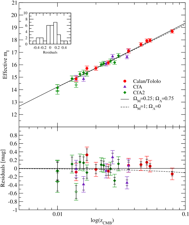
Figure 7: Effective $I$-band maximum vs redshift for the nearby supernovae of the Calan/Tololo, CfA and CfA2 sample. The data have been corrected for the stretch-luminosity relation and for Milky Way and host galaxy extinction. The r.m.s. along the concordance model line is $\sigma=0.17\pm 0.04$ mag. Subtracting the contribution of the average uncertainty, results in 0.13 mag estimated intrinsic dispersion (see text for details). SN 1998es and SN 1999dq were excluded from the fit (see text) and are plotted with open diamonds. The inset plots the histogram of the residuals.

4 High redshift supernovae

Next, we explore the possibility of extending the Hubble diagram to higher redshifts, where the effects of the energy density components of the universe are, in principle, measurable. The restframe $I$-band data available to date for this purpose are unfortunately very limited. They consist of only three supernovae (SN 1999Q, SN 1999ff and SN 2000fr) at redshift $z\sim 0.5$ observed in the near infrared (NIR) J-band collected during three different campaigns conducted using different facilities and by two different teams. Keeping all of these possible sources of systematic errors in mind, we include two of these supernovae in the $I$-band Hubble diagram.

4.1 SN 2000fr

SN 2000fr was discovered by the Supernova Cosmology Project (SCP) during a search for Type Ia supernovae at redshift $z\sim 1$ conducted in the $I$-band with the CFH12k camera on the Canada-France-Hawaii Telescope (CFHT) (Schahmaneche et al., 2001). The depth of the search allowed us to discover this $z\sim 0.5$ supernova during its rise, about 11 rest-frame days before maximum B-band light.

The supernova type was confirmed with spectra taken at the Keck II telescope and the VLT, showing that it was a normal Type Ia at $z=0.543$ (see Lidman et al. (2004); Garavini et al. (2005) for an extensive analysis of the spectrum). This supernova was followed in the restframe $B$, $V$ and $I$ bands involving both ground and space based facilities. Approximately one year later, when SN 2000fr had faded sufficiently, infrared and optical images of the host galaxy were obtained. The optical light curves in Knop et al. (2003) were re-fitted using the improved spectral templates for computing $k$-corrections. We found a $B$-band stretch factor of $s_{B}=1.034\pm 0.013$ and a time of $B_{\rm max}$, $t_{\rm max}=\rm MJD$ 51685.6. Restframe $B-V$ measurements at the time of $B_{\rm max}$ indicate that SN 2000fr did not suffer from reddening due to dust in the host galaxy (see Section 6 for a more extensive discussion). The adopted Milky Way reddening is $E(B-V)=0.030$ mag (Schlegel et al., 1998).

The near-infrared data were collected with ISAAC at the VLT. They consist of $J_{s}$-band observations during three epochs and a final image of the host galaxy without the SN (see Table 4). Each data point is composed of a series of 20 to 60 images with random offsets between exposures. Figure 8 shows a comparison between the Persson $J$ filter and the narrower ISAAC $J_{s}$ filter used for the observations, together with the atmospheric transmission, and the spectral template at maximum.

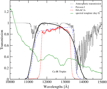
Figure 8: Comparison between the Persson $J$ filter (dashed-dotted line), the $J_{s}$ filter at ISAAC used for the observations of SN 2000fr (dashed line) and the $I$-band red-shifted to z=0.543 (heavy solid line). The atmospheric transmission is also plotted (dotted line). The spectral template at day 0 is on an arbitrary flux scale for readability purpose (solid line).

The advantage in using the narrower $J_{s}$ filter is that the transmission of the filter is not determined by the region of strong atmospheric absorption between 13500 and 15000 Å. Consequently, the zero-point is significantly more stable than that of standard $J$. This was very useful, because all the ISAAC data were taken in queue mode, where typically only one or two standard stars, chosen from the list of Persson et al. (1998), are observed during a night. All data, except the reference images, were taken during photometric nights and the difference in the zero-points from one night to the next was less than 0.01 magnitudes.

MJD	Epoch	$J_{s}$(mag)	$I$(mag)
51685.06	-0.33	22.50 $\pm$ 0.09	23.52 $\pm$ 0.10
51709.02	15.20	23.57 $\pm$ 0.22	24.52 $\pm$ 0.23
51731.96	30.07	23.14 $\pm$ 0.15	23.99 $\pm$ 0.16

Table 4: Summary of $J_{s}$-band data for SN 2000fr. The quoted errors are due to statistical Poisson noise and the uncertainty in the ZP (contributing 0.01 mag). Epochs are in restframe days relative to the date of $B$-band maximum. The restframe $I$-band is obtained through cross-filter $k$-correction from the observed $J_{s}$-band to Bessel $I$-band. The uncertainties also include the contribution from $k$-corrections, estimated to be 0.05 mag at all epochs considered.

The data were reduced using both internally developed routines and the XDIMSUM package in IRAF. The differences between the two analyses are within the quoted uncertainties. The supernova images were aligned with the host galaxy images and the flux scaled to the one with best seeing, using the field stars before performing PSF photometry (Fabbro, 2001). The results are presented in Table 4. The stated uncertainties include the statistical Poisson noise and the uncertainty on the estimate of the zero point, added in quadrature.

The $J_{s}$-band magnitude takes into account a colour term which arises from the difference between the $J$ filter of the standard star system and the $J_{s}$ filter used in ISAAC. This correction was small, $\sim$ 0.012 mag.

The cross-filter $k$-correction, $K_{IJ_{s}}$, to convert from $J_{s}$-band to rest-frame $I$-band, has been calculated following Kim et al. (1996) using the spectral templates improved for this work. The $k$-correction includes a term to account for the appropriate transformation between IR and optical photometric systems, equal to $(I-J)=0.03(\pm 0.02)$, determined by using the Vega magnitudes in $I$ and $J$ (Bessell et al., 1998; Cohen et al., 2003). We conservatively assume 0.05 mag total uncertainty in the $k$-corrections (see Section 2.2).

4.2 SN 1999ff

SN 1999ff was discovered by the High-Z Supernova Search Team (HZSST) during a search conducted at CFHT using the CFH12k camera in the $I$-band (Tonry et al., 2003). The supernova was confirmed spectroscopically as a Type Ia at redshift $z=0.455$. The adopted Milky Way reddening is $E(B-V)=0.025$ mag (Schlegel et al., 1998).

$J$-band observations, corresponding to restframe $I$-band, reported in Tonry et al. (2003), were taken at Keck using NIRC at two epochs only. The $J$-band filter that was used for these observations is very similar to the ISAAC $J_{s}$, shown in Fig. 8. We have used the published photometry, and, for consistency with the treatment of both the low redshift supernovae and SN 2000fr, we computed the $k$-corrections using the improved spectral templates. We found differences with the results published in Tonry et al. (2003), due to the use of an incorrect filter in the originally published results. (However, the $k$-corrections calculated as part of the MLCS distance fits to this object were done with the correct filter (Brian Schmidt, private communication)). The $I$-band magnitudes were also corrected for the offset found between the optical and IR systems, as explained in the previous section. The restframe $I$-band magnitudes obtained this way are reported in Table 5. The published optical $R$-band data were used to fit the restframe $B$-band light curve using the stretch method. Our time of maximum was within 1 day of the Tonry et al. (2003) value, with a best fit for the stretch $s_{B}=0.80\pm 0.05$.

$\rm MJD$	Epoch	I(mag)
51501.29	5.01	23.57 $\pm$ 0.11
51526.31	22.21	24.06 $\pm$ 0.24

Table 5: Summary of IR data for SN 1999ff. Epochs are in restframe days relative to the date of the $B$-band maximum ($t_{\rm max}={\rm MJD}51494.8$); restframe $I$-band magnitudes are computed applying $k$-corrections to the observed $J$-band data published in Tonry et al. (2003). The uncertainties also include the contribution from $k$-corrections, estimated to be 0.05 mag at all epochs considered.

4.3 SN 1999Q

SN 1999Q was discovered by the HZSST using the CTIO 4m Blanco Telescope and was spectrally confirmed to be a Type Ia SN at $z=0.46$ (Garnavich et al., 1999). The adopted Milky Way reddening is $E(B-V)=0.021$ magnitudes (Schlegel et al., 1998).

SN 1999Q was observed in the $J$-band over five epochs, the first with SofI on the ESO NTT and the following four with NIRC at the Keck Telescope (Riess et al., 2000). We recomputed the $k$-corrections using our new spectral template (as we did for SNe 2000fr and 1999ff) and we find a difference of up to 0.15 magnitudes between our $k$-corrections and those published in Riess et al. (2000).

A fit to the published restframe $I$-band data of SN 1999Q shows that it is a 4 standard deviation outlier in the $I$-band Hubble diagram. In order to investigate its faintness, we re-analysed the publicly available SofI data and found $J$=22.63 $\pm$ 0.15 mag, which is significantly brighter than the published value, $23.00\pm 0.14$ mag (Riess et al., 2000). Due to this large discrepancy, we decided to not include this SN in the rest of the analysis.

4.4 Light Curve fits for the high redshift supernovae.

The $I$-band light curves of the high redshift supernovae are not as well sampled in time as the low redshift sample analysed in Section 2. There are only few data points for each SN, making it impossible to perform the 5 parameter fit. Thus, we used the results of the fit of the local sample of supernovae to build a set of 42 $I$-band templates, which in turn have been used to fit the high redshift SN light curves.

The best fit light curve for each of the 42 supernovae in our low-redshift sample can be viewed as defining an $I$-band template. The high redshift supernovae are fit to each template with a single free parameter, $I_{\rm max}$, the absolute normalisation of the template. The time of $B_{\rm max}$ is obtained from the literature (SN 1999ff) or from our own $B$-band light curve fits (SN 2000fr). The best-fitting low-redshift $I$-band template fixes the date of the I-band maximum relative to the date of the $B$-band maximum. A $\chi^{2}$ comparison was used to choose the best low redshift template. Figs. 9 and 10 show the comparison of the data with the best fit template for each of the supernovae. Table 6 gives the results of the fit together with redshift, the number of data points, the template giving the best fit and the $\chi^{2}$. As there are only a few data points for each SN, the $\chi^{2}$ parameter has little significance for estimating the goodness of the fits. Thus, to estimate the possible systematic error in the measured peak magnitude from the selection of the light curve template, we computed the r.m.s. of the fitted $I_{max}$ of all the light curve templates satisfying $\chi^{2}\leq\chi_{min}^{2}+3$. This possible systematic uncertainty is reported also in Table 6. For both SNe this is quite small, and compatible with the scatter due to the statistical uncertainties, thus, it is a conservative estimate.

Figure 9: $I$-band fit for SN 2000fr. Out of 42 $I$-band templates, the best fit was obtained with the template of SN 1992bc. The fit was performed with only one free parameter, the peak magnitude, $I_{\rm max}=23.48\pm 0.08$ mag. Supplemental data from the $B$-band (not shown) is used to fix the date of $B$-maximum.

Figure 10: $I$-band fit for SN 1999ff. Out of 42 $I$-band templates, the best fit was obtained with the template of SN 1996bl. The fit was performed with only one free parameter, the peak magnitude, $I_{\rm max}=23.55\pm 0.10$ mag. Supplemental data from the $B$-band (not shown) is used to fix the date of $B$-maximum.

SN	$z$	$s_{B}$	$n$	$I_{\rm max}$	template	$\chi^{2}$	$A_{J}^{MW}$
SN 2000fr	0.543	1.034 $\pm$ 0.011	3	23.48 $\pm$ 0.08 $\pm$ 0.04	SN 1992bc	1.04	0.027
SN 1999ff	0.455	0.80 $\pm$ 0.05	2	23.55 $\pm$ 0.10 $\pm$ 0.08	SN 1996bl	0.05	0.022

Table 6: List of the high redshift Type Ia SNe used in this work. Columns are: IAU name, redshift, number of data points used in the fit, magnitude of the peak resulted from the fit (both statistical and systematic uncertainties are given) before Milky Way extinction correction, best fit template, $\chi^{2}$ of the fit, Milky Way extinction in the $J$-band.

4.5 Monte-Carlo test of the fitting method

A Monte-Carlo simulation was run in order to test the robustness of the fitting method applied to the high redshift SNe. The measurement uncertainties were used to generate a set of 1000 SNe, with data points randomly distributed around the real data and at the same epochs as the data. All the simulated data sets were in turn fitted with the 42 templates and the one giving the minimum $\chi^{2}$ was selected for each simulation. The distribution of the fitted parameters in each of the simulated data sets around the true values, fitted on the experimental data, was studied to check for systematic uncertainty in the fitting procedure. This was found to be robust, always selecting the same template as the one giving the best fit for both SNe. No bias was found, therefore confirming the peak magnitude fitted with this method. The uncertainty in $I_{\rm max}$ reported in Table 6 was consistent with the dispersion in the distribution of $I_{\rm max}$ measured from the simulations.

5 The $I$-band Hubble diagram up to $z\sim 0.5$

The $I$-band peak magnitudes of the high redshift supernovae reported in Table 6 were corrected for Milky Way extinction. Note that both SN 1999ff and SN 2000fr have been reported not to suffer from extinction from their host galaxies.

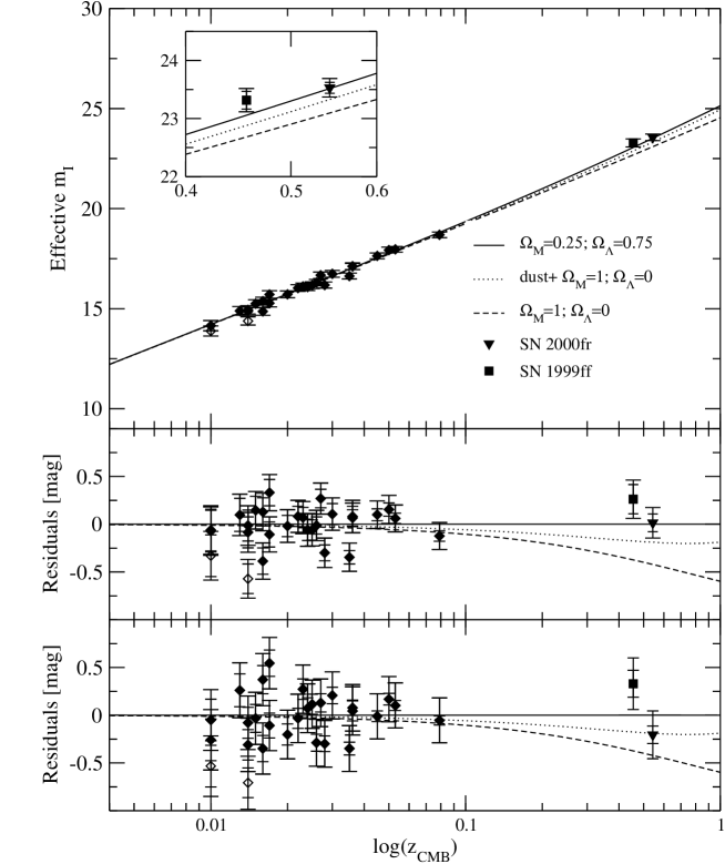
Figure 11: Effective $I$-band maximum versus redshift for the nearby supernovae of the Calan/Tololo, CfA and CfA2 sample, together with two supernovae at redshift $\sim 0.5$ for case $c$ (top panel), residuals to the ($\Omega_{M},\Omega_{\Lambda}$)=(0.25,0.75) model for case $c$ (middle panel) and case $a$ (bottom panel). SN 1998es and SN 1999dq were excluded from the fit (see text) and are plotted with open diamonds. Only the low-redshift SNe have been extinction corrected. The host galaxy extinction correction would make the two high-redshift data points closer to each other but with larger error bars.

The Hubble diagram has been built both with and without width-luminosity correction (case $c$ and case $a$ respectively), where the systematic uncertainties on the peak magnitudes of the distant supernovae, listed in Table 6, are added in quadrature to the statistical uncertainties. Cases $b$ and $d$ are like $a$ and $c$ but neglect the systematic uncertainties from Table 6. Figure 11 shows the extended Hubble diagram (case $c$), where an intrinsic uncertainty of 0.13 mag has been added in quadrature to the measurement errors of the plotted data. The solid line represent the best fit to the nearby data for the concordance model $\Omega_{M}=0.25$ and $\Omega_{\Lambda}=0.75$. Also plotted is the model for $\Omega_{M}=1$ and $\Omega_{\Lambda}=0$ (dashed line), and a flat, $\Lambda=0$ universe in the presence of a homogeneous population of large dust grains in the intergalactic (IG) medium able to explain the observed dimming of Type Ia SNe at $z\sim 0.5$ in the $B$-band (dotted line) (Aguirre, 1999a, b). The bottom panel shows the residuals obtained for case $a$. Table 7 lists the $\chi^{2}$ values for the high redshift SNe for each of the models. The $\Omega_{\Lambda}$-dominated cosmology is formally favored over the other two models at the $>$2$\sigma$ level. However, two high redshift supernovae obviously do not provide the full gaussian distribution that would confirm this result.

$(\Omega_{M},\Omega_{\Lambda})$	$\chi^{2}_{a}$	$\chi^{2}_{b}$	$\chi^{2}_{c}$	$\chi^{2}_{d}$
(0.25,0.75)	2.18	2.36	1.16	1.44
(1,0)	7.56	8.44	15.56	18.30
$(1,0)_{dust}$	3.52	3.96	5.36	6.48

Table 7: $\chi^{2}$ (for 2 dof) of each model to the high redshift data, without stretch correction and with systematic uncertainties added in quadrature ($\chi^{2}_{a}$), neglecting the systematic uncertainties ($\chi^{2}_{b}$), with stretch correction and adding the systematic uncertainties in quadrature ($\chi^{2}_{c}$) or neglecting them ($\chi^{2}_{d}$).

Systematic uncertainties in the method used here also cannot be extensively explored with only two supernovae. Some uncertainties are specific to the sample considered here. The different fitting methods applied to the restframe $I$-band light curve for the low and high redshift samples can be easily overcome if distant supernovae are followed at NIR wavelengths with better time coverage. Both the low and high redshift samples used in this analysis are rather heterogeneous, as they were collected from different data sets. Future data sets collected with a single instrument would naturally solve this problem.

6 SN Ia colours and intergalactic dust

Multi-colour photometry allows one to search for non-standard dust having only a weak wavelength dependence, such as a homogeneous population of large grain dust, as proposed by Aguirre (1999a, b).

If we assume that grey dust is responsible for the dimming of SNe Ia in the $B$-band at $z\sim 0.5$, we can calculate the expected extinction in other filters and compute the resulting colours. Following Goobar et al. (2002a), we use the SNOC Monte-Carlo package (Goobar et al., 2002b) for two cases of the total to selective extinction ratio - $R_{V}=4.5$ and $9.5$. We assume that the dust is evenly distributed between us and the SNe in question and we assume a flat cosmological model with a zero cosmological constant.

The measured $B-I$ and $B-V$ colours of SN 1999ff and SN 2000fr, corrected only for Milky-Way extinction, are presented in Tables 8 and 9 and plotted in figure 12. The error bars include the contribution of the intrinsic colour dispersion. The expected evolution in the $B-I$ and $B-V$ colours of an average SNe Ia in the concordance model and in the two models with grey dust and without a cosmological constant at $z=0.5$ are also shown.

The $\chi^{2}$ has been computed for both $B-V$ and $B-I$ evolution for SN 1999ff and SN 2000fr, and for both supernovae together (see Table 10). The correlations between SN colours at different epochs found in (Nobili et al., 2003) were taken into account. However, we note that, although this correlation should be taken into account in the calculations, neglecting it would not change significantly the conclusions of the analysis. Although individual supernovae give $\chi^{2}$ values that would seem to distinguish between the models, the combined results disfavour such conclusions.

Epoch	$B-I$
SN 2000fr
-0.32	-0.51 $\pm$ 0.12
14.70	-0.50 $\pm$ 0.24
29.08	1.42 $\pm$ 0.17
SN 1999ff
5.59	-0.18 $\pm$ 0.13
27.20	1.38 $\pm$ 0.24

Table 8: Restframe $B-I$ colours in magnitudes for the two high redshift SNe. The Epoch is in restframe days relative to the $B$-band maximum, divided by the $B$-band stretch.

Epoch	$B-V$
SN 2000fr
-7.97	-0.06 $\pm$ 0.05
-3.51	-0.14 $\pm$ 0.05
4.60	-0.12 $\pm$ 0.05
12.93	0.24 $\pm$ 0.08
20.31	0.61 $\pm$ 0.07
30.22	0.99 $\pm$ 0.09
SN 1999ff
-7.99	0.03 $\pm$ 0.08
1.91	-0.02 $\pm$ 0.09
1.98	0.10 $\pm$ 0.12
2.91	0.23 $\pm$ 0.12
19.55	0.71 $\pm$ 0.09
28.75	1.22 $\pm$ 0.20

Table 9: Restframe $B-V$ colours in magnitudes for SN 1999ff and SN 2000fr. The Epoch is in rest frame days relative to the $B$-band maximum, divided by the $B$-band stretch.

Figure 12: The evolution in the colour of SN 1999ff (squares) and SN 2000fr (triangles), $B-V$ (top panel) and $B-I$ (bottom panel), compared to the colour evolution of the average SNe Ia in a $\Lambda$ dominated universe (solid line) and a $\Omega_{M}=1$, $\Omega_{\Lambda}=0$ universe with presence of grey dust with $R_{V}$=4.5 (dashed line) and $R_{V}$=9.5 (dotted line) for $z=0.5$.

To make our test for grey dust more effective, a different approach was followed. The method of least squares has been used to combine colour measurements along time for each supernova (see Cowan, 1998, p.106 for details). The residuals between the data and the models are averaged with a weight that is determined from the covariance matrix. In the following, we refer to $E(X-Y)$ to describe the colour excess of any supernova with respect to the average $X-Y$ colour of nearby SNe Ia, as derived in (Nobili et al., 2003). First we applied this method to all local supernovae and used the results to establish the expected distribution in the $E(B-I)$ vs $E(B-V)$ plane, as showed in Fig. 13.

As the high redshift SNe were not corrected for host galaxy extinction, we computed the colour distribution of nearby SNe Ia for two cases: the left-hand panels represent the distribution of colour excess of 27 nearby SNe not corrected (top panel) and corrected (bottom panel) for host galaxy extinction. Spectroscopically peculiar SNe have been excluded from the analysis. The projection of the ellipses on each colour axis is the estimated standard deviation in that colour and the inclination is defined by the linear Pearson correlation coefficient computed on the same data sample. The solid contours represent 68.3%, 95.5% and 99.7% probability.

The right-hand panels in Fig. 13 show the combined values of colour excess, $[E(B-V),E(B-I)]$, for the high redshift supernovae: $[0.12\pm 0.09,0.25\pm 0.17]$ for SN 1999ff and $[-0.11\pm 0.08,-0.10\pm 0.18]$ for SN 2000fr. These are compared to the local supernova distribution (solid lines), that represent the distribution expected in the absence of IG dust. Also plotted is the 68.3% level of the expected distribution in presence of grey dust with $R_{V}=9.5$, represented by the ellipse (dashed line) that is displaced by (0.06,0.19) from the no-dust model. Only the case of $R_{V}=9.5$ has been plotted for readability reasons, given the small difference between the two dust models. Note that this is the closer to the no-dust model. The ellipse corresponding to $R_{V}=4.5$ would be displaced by (0.03,0.04), respectively in $E(B-V)$ and $E(B-I)$, from the $R_{V}=9.5$ model.

We computed the $\chi^{2}$ of the high redshift data for all three models, for two cases: in the first case, the nearby SNe Ia are corrected for extinction by dust in the host galaxy, and, in the second case, they are not (bottom and top panels of Fig. 13). For each model, we sum the $\chi^{2}$ contribution from all SNe, taking into account the correlation found between $E(B-V)$ and $E(B-I)$ in the nearby sample. In the first case, the reduced $\chi^{2}$ (for 4 degrees of freedom) are 0.63, 1.20, and 0.97 for the no-dust, IG dust with $R_{V}=4.5$ and IG dust with $R_{V}=9.5$ models respectively. In the second case, the reduced $\chi^{2}$ are 0.62, 1.55 and 1.32 respectively. We note that both the intrinsic dispersion in the colours of the nearby data, and the uncertainties in the colours of the high redshift SNe, have been taken into account in computing the $\chi^{2}$. The statistical significance of these results is very limited, and should only be taken as an example of the method developed here. Moreover, the possibility for this analysis to be affected by systematic effects is not negligible. Increasing the sample and the time sampling for each object would allow us not only to improve the significance of our statistic, but it will also be a means to identify and quantify systematic effects involved.

A Monte Carlo simulation was used to estimate the minimum sample size needed to test for the presence of homogeneously distributed grey dust in the IGM. SNe colours were generated following the binormal distribution defined by the nearby SNe Ia sample. Under the assumption that the systematic effects are negligible and an average measurement uncertainty of 0.05 mag in both $E(B-V)$ and $E(B-I)$, we found that a sample of at least 20 SNe would be needed to exclude the IG dust model with $R_{V}=9.5$ at the 95% C.L. Note that the average measurement uncertainty of 0.05 mag can be achieved with different strategies. Currently, the uncertainties on the individual measurements give the main contribution to the colour uncertainties. A good sampling would allow us to better identify and quantify currently unidentified systematic effects which may possibly be affecting the current analysis.

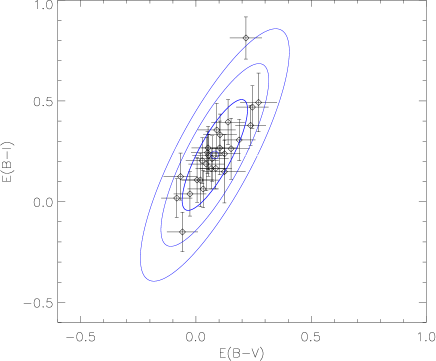
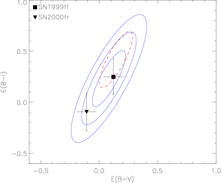
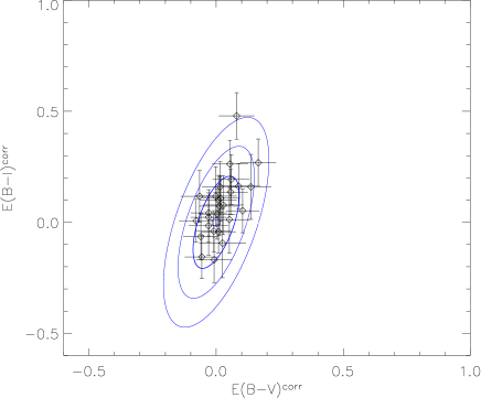
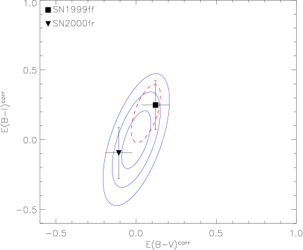
Figure 13: Left-hand panels: distribution of combined colour measurements of nearby SNe Ia in the $E(B-I)$ vs $E(B-V)$ plane, not corrected (top panel) and corrected (bottom panel) for the host galaxy extinction. The solid contours incorporate 68.3%, 95.5% and 99.7% of the sample. Right-hand panels: SN 1999ff and SN 2000fr compared to the distribution defined by nearby SNe in the case of no IG dust (solid ellipses), and in the case of IG dust with $R_{V}=9.5$ (dashed ellipse). For clarity only the 68.3% level has been plotted for the dust distribution.

	$\chi^{2}_{B-V}$/dof	$\chi^{2}_{B-I}$/dof
SN 2000fr
no dust, $(\Omega_{M},\Omega_{\Lambda})$=(0.25,0.75)	2.33/4	2.08/3
dust $R_{v}=9.5$, $(\Omega_{M},\Omega_{\Lambda})$=(1,0)	4.24/4	3.94/3
dust $R_{v}=4.5$, $(\Omega_{M},\Omega_{\Lambda})$=(1,0)	5.29/4	4.50/3
SN 1999ff
no dust , $(\Omega_{M},\Omega_{\Lambda})$=(0.25,0.75)	6.05/5	3.93/2
dust $R_{v}=9.5$, $(\Omega_{M},\Omega_{\Lambda})$=(1,0)	4.69/5	2.06/2
dust $R_{v}=4.5$, $(\Omega_{M},\Omega_{\Lambda})$=(1,0)	4.31/5	1.89/2
SNe combined
no dust , $(\Omega_{M},\Omega_{\Lambda})$=(0.25,0.75)	8.38/9	6.01/5
dust $R_{v}=9.5$, $(\Omega_{M},\Omega_{\Lambda})$=(1,0)	8.93/9	6.00/5
dust $R_{v}=4.5$, $(\Omega_{M},\Omega_{\Lambda})$=(1,0)	9.59/9	6.39/5

Table 10: $\chi^{2}$ computed for the 3 different models and colours for each of the supernovae and for their combination.

7 Test for SN brightness evolution

Evolution of the properties of the progenitors of SNe Ia with redshift has often been proposed as an alternative explanation for the observed dimming of distant SNe. This is based on the assumption that older galaxies show different composition distribution than younger ones, e.g. an increased average metallicity, resulting in different environmental conditions for the exploding star. A simple way to test for evolution is to compare properties of nearby SNe with distant ones. This will not prove that there is no evolution, but it will exclude it on a supernova-by-supernova or property-by-property basis, always finding counterparts of distant events in the local sample.

In this work we compared the colours of nearby and distant supernovae (primarily to test presence of “grey” dust). Although the size of the high redshift sample is very limited, our results do not show any evidence for evolution in the colours of SNe Ia. Furthermore, the correlation found between the intensity of the secondary peak of $I$-band light curve and the supernova luminosity give an independent way of testing for evolution. The restframe $I$-band light curve of the high redshift supernovae were all best fitted by templates showing a prominent second peak, i.e. inconsistent with the intrinsically underluminous supernovae. Note that the data presented here for SN 2000fr show for the first time a case where the secondary peak is unambiguously evident in the data even prior to the light curve fit. Table 11 lists the $\Delta\chi^{2}$ for the fit of the high redshift SNe to the templates of the two underluminous SN 1991bg and SN 1997cn, relative to the best fit. The $\chi^{2}$ values are significantly larger than the best fit value.

	$n$	SN 1991bg	SN 1997cn
SN 2000fr	3	24.03	21.73
SN 1999ff	2	3.28	2.72

Table 11: $\Delta\chi^{2}$ for the fit of the high redshift SNe to the templates of the two underluminous SNe relative to the best fits (which are “normal” SN templates). $n$ is the number of data points used in the one-parameter fit (see discussion in section 4.4).

8 Summary and conclusions

In this work we have investigated the feasibility and utility of using restframe $I$-band observations for cosmological purposes.

We have developed a five parameter light curve fitting procedure which was applied successfully to 42 nearby Type Ia supernovae. The fitted light curves were used to build a set of templates which include a broad variety of shapes. We have found correlations between the fitted parameters, in particular between the time of the secondary peak and the $B$-band stretch, $s_{B}$. Moreover, a width-luminosity relation was found between the peak $I$-band magnitude and the $B$- and $I$-band stretches ($s_{B}$ and $s_{I}$).

We built a restframe $I$-band Hubble diagram using 26 nearby supernovae at redshifts $0.01\leq z\leq 0.1$, and measured an r.m.s. of 0.24 mag, smaller than the uncorrected dispersion corresponding to restframe $B$-band. The width-luminosity relation was used to reduce the r.m.s. to 0.17 $\pm$ 0.03 mag (including measurement errors), corresponding to an intrinsic dispersion of 0.13 mag. Differences between the three data samples are also discussed.

$J$-band measurements of one new high redshift supernova plus published data of another were used to extend the Hubble diagram up to $z\sim 0.5$. The restframe $I$-band light curves of the $z\sim 0.5$ supernovae were fitted with templates that were built from the nearby SNe Ia, as the five parameter fit method could not be used for the poorly sampled high redshift light curves. The peak $I$-band magnitude of the high redshift SNe was compared to three different sets of cosmological parameters. The “concordance model” of the universe, ($\Omega_{M},\Omega_{\Lambda}$)=(0.25,0.75), is formally found in better agreement with the data than the other models at the $>$2$\sigma$ level. However, the small sample size does not yet allow strong conclusions to be drawn.

Alternative explanations for the observed dimming of supernova brightness, such as the presence of grey dust in the IG medium or evolutionary effects in the supernova properties have also been addressed. Both the $I$-band Hubble diagram and multi colour photometry have been used for testing grey dust. Although no firm limits on the presence of grey dust could be set, this study shows that with higher statistics, the restframe $I$-band measurements could provide useful information on cosmological parameters, including tests for systematic effects. A Monte Carlo simulation indicates that a sample of at least 20 well observed SNe Ia would be enough for setting limits through the multi-colour technique used in this paper. A similar technique, using QSO instead of SNe Ia, was successfully used by Mörtsell & Goobar (2003) to rule out grey dust as being the sole explanation for the apparent faintness of SNe Ia at $z\sim 0.5$.

Possible systematic uncertainties affecting the restframe $I$-band Hubble diagram are discussed. Some sources are identified, for instance the different methods applied for fitting the low and the high redshift samples, selection effects for bright objects due to the limiting magnitude of the search campaign, as well as uncertainties in the $k$-correction calculations due to the presence of the Ca IR triplet feature in the near infrared region of the SN spectra. However, these systematic uncertainties differ from the ones that could affect the restframe $B$-band Hubble diagram.

Restframe $I$-band observations of distant SNe Ia are feasible, useful and complementary to the already well established observations in the $B$-band.