Efficient Monte Carlo methods for continuum radiative transfer

We discuss the efficiency of Monte Carlo methods in solving continuum radiative transfer problems. The sampling of the radiation field and convergence of dust temperature calculations in the case of optically thick clouds are both studied. For spherically symmetric clouds we find that the computational cost of Monte Carlo simulations can be reduced, in some cases by orders of magnitude, with simple importance weighting schemes. This is particularly true for models consisting of cells of different sizes for which the run times would otherwise be determined by the size of the smallest cell. We present a new idea of extending importance weighting to scattered photons. This is found to be useful in calculations of scattered flux and could be important for three-dimensional models when observed intensity is needed only for one general direction of observations. Convergence of dust temperature calculations is studied for models with optical depths $\tau_{\rm V}=10-10^{4}$. We examine acceleration methods where radiative interactions inside a cell or between neighbouring cells are treated explicitly. In optically thick clouds with strong self-coupling between dust temperatures the run times can be reduced by more than one order of magnitude. The use of a reference field was also examined. This eliminates the need for repeating simulation of constant sources (e.g., background radiation) after the first iteration and significantly reduces sampling errors. The applicability of the methods for three-dimensional models is discussed.

1 Introduction

Continuum radiative transfer problems are commonly solved with Monte Carlo calculations. The radiation field is simulated according to the actual processes that are assumed to be taking place in an interstellar cloud. Emission from background, internal sources, and the dust itself is represented by a number of photons packages, each corresponding to a large number of actual photons at one wavelength. Random numbers determine the initial positions and directions of the photon packages. The distance to a point where scattering takes place and the direction after scattering are also calculated using random numbers. This is the basic scheme in studies of light scattering (e.g., Mattila mattila70 (1970); Witt witt77 (1977)). In scattering, the probability distribution for the change of photon direction is given by the scattering function that depends on dust properties. It is this random change of direction that precludes (with the exception of isotropic scattering or pure forward scattering) the use of direct ray tracing methods which are often used in line transfer. If, in addition to scattered light, also dust emission is to be solved then during the simulation the number of absorbed photons must be registered in each cell of the model cloud. This could be done at each position where scattering takes place but unless optical depth is very high (or one is calculating only the scattered flux) it is better to explicitly calculate absorptions in all cells that the photon package passes through. Especially in optically thin clouds the statistics of absorbed energy would otherwise remain very poor.

Monte Carlo continues to be the standard method for the modelling of dust emission from interstellar clouds (Bernard et al. bernard92 (1992); for recent papers see, e.g., Stamatellos & Whitworth stamatellos (2003); Concalves et al. concalves (2004); Niccolini et al.niccolini (2003); Juvela & Padoan juvela03 (2003); Pascucci et al. pascucci (2004) and references therein; Kurosawa et al. kurosawa04 (2004); Whitney et al. whitney03 (2003); Wolf et al. wolf03 (2003)). Several methods can be employed to improve the sampling. One of the most common is the method of forced first scattering (e.g., Mattila mattila70 (1970)) which improves sampling of scattered flux in clouds of low optical depth. In an optically thin cloud most photons pass through the cloud unscattered and give no information on scattered flux. Forced scattering means that one calculates for each package the fraction of photons that do scatter in the cloud. Unscattered photons are followed through the cloud along the original direction while the calculated fraction is always scattered somewhere along the way. The distance to the point of scattering is calculated from a conditional probability distribution ’where will the photon package scatter if it does scatter before exiting the cloud’.

In optically thick clouds most of the incoming flux is scattered many times and a photon package does not usually propagate very far. In a spherically symmetric model this means that very few background photon packages reach the cloud centre. In order to get proper sampling in optically thick regions the number of simulated photon packages must be extremely large, and the run times become correspondingly very long. Niccolini et al. (niccolini (2003); method 2) presented a partial solution which is analogous to the method of forced scattering but where the roles of the scattered and unscattered flux are reversed. The fraction of photons that does not scatter is first calculated and that part of the photon package is followed through the cloud toward the original direction. Rest of the photons is scattered somewhere along the way. The procedure is repeated after each scattering. While the method of forced scattering gives (in statistical sense) the right amount of scattered flux it is not equally clear that the method of Niccolini et al. (niccolini (2003)) always provides correct estimates of absorbed photons. If the number of simulated photon packages is small the flux observed in cloud centre consist only of photons that are first scattered a few times near the surface and after this propagate unscattered to the centre. It remains open what is the ratio of these photons and those in the more rare photon packages (not necessarily more rare photons) that reach the centre only after many scatterings. At the limit of high optical depth for scattering and low optical depth for absorption the method would appear to improve the sampling but actually all flux in the centre should still result from packages that have scattered numerous times, i.e. the method could not decrease the number of photon packages needed in the simulation. These are, of course, not faults of the method itself but are simply consequences of the sampling problem. The method does not address problems arising from different cell sizes and, therefore, while this method is probably very useful in many cases it is not yet a complete solution to the problem.

One of the main advantages of Monte Carlo methods is their great flexibility in the way radiation field is sampled. All probability distributions employed in the simulation of photon packages can be modified as long as these are compensated by corresponding changes in the weighting, i.e. the number of actual photons in a package. For some reason this advantage is often not used and simulations are unnecessarily inefficient. High optical depths are perceived to pose another problem and not only because of difficulties in the sampling of the radiation field. In an optically thick cloud there may be significant self-coupling between dust temperatures. In the usual scheme this means that dust temperatures can not be solved directly and one is forced to iterate between simulation of the radiation field and updating of dust temperature estimates. The number of iterations depends on the optical depth, $\tau$. For a cloud where $\tau$ reaches at optical wavelengths several hundred run times can become orders of magnitude longer than in the case of an optically thin cloud. This depends, however, very much on the external radiation field and the dust temperatures. According to Bernard et al. (bernard92 (1992)), for cold clouds embedded in normal interstellar radiation field the dust coupling is unimportant unless optical depth is several hundred. This was confirmed by Concalves et al. (concalves (2004); see their Fig. 1) but the situation can be very different in the presence of hot dust.

The slow convergence at high optical depths is, of course, not related to the Monte Carlo method per ce. Even if radiation field is sampled with Monte Carlo method the dust temperatures can be solved without iterations and even if iterations are made, simulation of the radiation field need not be repeated. Because of the larger memory requirements such schemes are, however, practical only for one-dimensional models. Bjorkman & Wood (bjorkman01 (2001)) presented a modification where local dust temperature is updated after each absorption and a new photon is immediately re-emitted from the same position. The frequency of the emitted photon is obtained from a probability distribution that takes into account both the previously emitted photons and the correction due to the updated temperature. The desired noise level determines the number of required photon packages and once these and the induced re-emitted photons have been simulated the calculations provide a converged solution. The authors state that the method does not suffer from convergence problems associated with $\Lambda$-iteration methods. We return to this question later in the paper.

In this paper we will study the efficiency of Monte Carlo radiative transfer calculation. We will discuss separately efficient sampling of the radiation field and convergence of iterations. One-dimensional, i.e. spherically symmetric model clouds are used as examples. We will, however, emphasise that most results can be directly transferred to three-dimensional cloud modelling and we will briefly discuss the applicability of the methods in the case of 3D models containing millions of cells. In Sect. 2 we describe the program and the implementation of weighting, reference field and convergence acceleration schemes. Results from tests with one-dimensional models are presented in Sect. 3, and the results are discussed in Sect. 4

2 The program

In this section we present some details of our implementation of the radiative transfer program. More specifically, we discuss the possibilities of improving the sampling of the radiation field so that a given accuracy of the results can be obtained with a smaller number of photons packages. On the other hand, we will discuss the convergence of dust temperature calculations in the case of optically thick clouds. This part of the discussion does apply equally to programs where some method other than Monte Carlo is used to estimate the radiation field.

2.1 Sampling of the radiation field

One of the main advantages of Monte Carlo methods is that the sampling can be easily adapted according to the problem at hand. This possibility is, however, seldom used and, in order to ensure proper sampling in all parts of the model, simulations need an exceedingly large number of photon packages. This adaptation or ‘weighting’ is what in Monte Carlo integration would be called importance sampling. While it may be possible to create adaptive methods (analogous to stratified sampling; see Press et al. press_nr (1992)) we restrict our discussion to more simple schemes.

In normal Monte Carlo simulation photon packages are created at random locations (within emitting medium or on the surfaces of separate radiation sources) and sent uniformly toward random directions. Each package has equal weight i.e. the number of true photons is divided evenly between created packages. One is not restricted to the use of uniform spatial and angular distributions and one could, e.g., send twice as many photon packages from certain part of the cloud provided that each of these packages contains only half of the original number of photons. More generally, if one assumes a new probability distribution $p(r,\Omega)$ for positions $r$ and directions $\Omega$ of the created photon packages the weight of the photon package is

$$W_{i}=\frac{1}{p(r_{i},\Omega_{i})}.$$ (1)

The default number of photons included in a package is multiplied with this number where $r_{i}$ and $\Omega_{i}$ are the actual position and direction of the photon package. Weighting can be applied to background photons, photons emitted by dust inside the cloud and for each discrete source included in the model. In each case the spatial and angular distributions can be weighted separately. The four weighting schemes used in this paper ($A$, $B$, $C$, and $D$) are illustrated in Fig. 1. These are are discussed below and a more detailed presentation can be found in Appendix A.2.

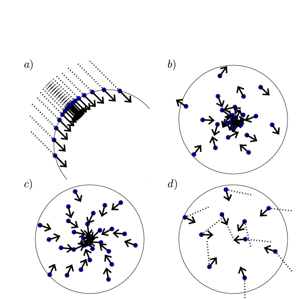
Figure 1: The four weighting schemes ($A$, $B$, $C$, and $D$) used in the Monte Carlo simulations in this paper. The figures illustrate a case where the sampling is improved in the centre of a spherically symmetric model cloud: background packages are sent preferentially towards the cloud centre (scheme $A$), more photon packages are created in the inner parts (scheme $B$), within the cloud photon packages are sent preferentially towards the cloud centre (scheme $C$), and scattered photon packages are directed preferentially towards the cloud centre (scheme $D$).

2.1.1 External radiation field: weighting scheme $A$

In a spherically symmetric cloud all background photon packages enter the outermost shell but, because of their smaller diameter, the inner shells are hit by relatively few packages. At least in optically thin clouds the problem can be alleviated by sending photon packages preferentially toward cloud centre. The original probability distribution of the impact parameter, $p(d)\propto d$, can be replaced one with higher probability at small values of $d$ (e.g., $p(d)\propto d^{\alpha}$ with $\alpha<1$). We use a scheme where the same number of photon packages is sent towards each annulus as defined by the radial discretization (weighting scheme $A$). Within each annulus we have the usual distribution of $p(d)\propto d$. The number of photon packages is fixed for each annulus and the random noise is reduced. This is, however, not yet optimal. In an optically thin model with $N$ shells each photon package enters the outermost shell but only one in $N$ hits the innermost cell. A more strongly peaked probability distribution could result in more uniform errors.

2.1.2 Internal radiation field: weighting scheme $B$

Different cell sizes also affect the sampling of dust emission within the cloud. This is particularly problematic in optically thick clouds where self-coupling between dust temperatures is strong. In a spherical model the the innermost cells can be orders of magnitude smaller than the the outermost shells. Sampling errors increase toward centre and the number of required photon packages depends directly on the size of the smallest cells. The solution is similar as in the case of background photons. Emissions take place at random positions with radial probability distribution, $p(r)\sim r^{2}$. For photon packages this can be replaced with a steeper distribution (e.g., $p(r)\sim r^{\beta}$ with $\beta$ below 2). We use a procedure where the same number of photon packages is generated in each cell but the locations within the cells follow the $p(r)\sim r^{2}$ distribution (weighting scheme $B$). In extremely optically thick clouds one might also consider whether photon packages should be created preferentially close to cell boundaries so that these would better sample the energy transfer between cells. The importance of different cells as sources of radiation could also be taken into account and more packages could be sent from denser and warmer cells.

2.1.3 Angular distribution of photons created in the cloud: weighting scheme $C$

In order to improve the sampling of the smallest cells we consider weighting the angular distribution of photon packages created within the cloud. Uniform angular distribution is replaced with distribution that peaks in the direction of the cloud centre or, more generally, toward any region where sampling is to be improved. We use an exponential function $p(\theta)\propto e^{-\gamma\theta}$ where $\theta$ is angular offset from the direction of the cloud centre and $\gamma$ is a positive constant (weighting scheme $C$). The exponential function is convenient since the inverse cumulative probability density function, $P^{-1}$ , is easily calculated and can be used to generate angles from the selected distribution. However, the calculation of the $P^{-1}$ can be replaced with a lookup to a table of $P$-values and, in practise, there are no restrictions for using any function as the probability distribution $p$.

2.1.4 Place and angular distribution of scattering: weighting scheme $D$

In weighting scheme $D$ we apply weighting to scattered photons. The method of forced first scattering would be one example of this (see Sect. A.1). Here we are, however, more interested in the angular distribution of the scattered photons. The goal can be to increase the flux of packages (not photons!) toward optically thick parts of the cloud or toward one particular direction from which the emerging scattered intensity is observed. Scattered photons already have a non-uniform probability distribution, $p(\Omega)$, which is determined by scattering function of the dust model. This can be given by the Henyey-Greenstein (henyey41 (1941)) formula, or some other function specified in analytical or tabular form. The distribution $p$ is defined in a coordinate system that is fixed by the initial direction of the photon package. Let us assume that we want to have locally a probability distribution $q(\Omega)$ for the directions of scattered photon packages. Random directions are generated according to this distribution and each package is weighted with the ratio

$$W_{i}=\frac{p(\Omega^{\prime})}{q(\Omega)}.$$ (2)

Functions $p$ and $q$ are defined in different coordinate systems and one must apply a rotation to find out what direction $\Omega^{\prime}$ the selected direction $\Omega$ corresponds to.

The presented scheme clearly works if one divides a photon package into $n$ small packages, each containing a fraction $\propto p(\Omega^{\prime})/q(\Omega)$ of the original number of photons and having directions following the distribution $q$. For practical reasons it is not possible to split a package this way. One can, however, use the scheme without creating any new photon packages. When a package is scattered the new direction is obtained from the probability distribution $q$ and the number of photons contained in the package is multiplied by the factor given by Eq. 2. The weight $W_{i}$ can be smaller or larger than one and for some photon packages the number of photons can actually increase. The result is, of course, correct only statistically and after the simulation of many photon packages. The possibility of weighting leads to an interesting conclusion that all frequencies can be calculated simultaneously using a single photon package. Each time scattering occurs the number of photons at each frequency is multiplied by a factor depending on the realised scattering angle and the scattering function at that frequency. Weighting should also be applied according to the distance between scatterings which depends on the frequency-dependent opacity of the medium. Since this is very wavelength dependent such a scheme would, however, most likely result in increased sampling errors.

The method $D$ is not the same as the ’peeling off’ method of Yusef-Zadeh et al. (yusef94 (1994)) that is used to improve the quality of images of scattered light (Wood & Reynolds wood99 (2003); Whitney et al. whitney03 (2003)). In the ’peeling off’ method one calculates and registers after each scattering the fraction of photons that are scattered towards the observed and escape the cloud. The angular distribution (or weighting) of the rest of the photons still essentially follows the original scattering function. Therefore, the sampling of the scattered flux remains unchanged within the cloud while in our method $D$ it is changed. Method $D$ improves the sampling of the observed scattered flux by increasing the number of regular photon packages that exit the cloud towards the observer. The ’peeling off’ method is more efficient if only emerging flux is considered and only for one single direction. Method $D$ might be competitive in cases where observed flux results from multiple scatterings in an optically thick medium. Because method $D$ improves sampling in the selected general direction it can also be used when images of the scattered flux are needed for several directions close to each other. Of course, it would be possible to combine the two methods. Method $D$ would be used to modify sampling within the cloud and the ’peeling off’ could still be performed after each scattering. This possibility is not studied any further in this paper.

2.2 Reference field

In Monte Carlo integration errors are proportional to function values. If solution is known for a reference function that is similar to the integrated function only the difference needs to be solved with Monte Carlo methods and the errors are proportional to the difference between the actual function and the reference. This idea was first applied to line transfer calculations by Bernes (bernes79 (1979)). He assumed a reference field corresponding to a fixed excitation temperature and Monte Carlo simulation was used to determine the differences between the true field and the constant reference field. Choi et al. (choi (1994)) improved the method by using the solution from the previous iteration as the reference. As the reference field approaches the true field the sampling errors decrease on each iteration.

So far a reference field has not been used in connection with dust emission calculations. The implementation is, however, straightforward. The reference field is taken to correspond to the situation of the previous iteration. On the first iteration reference field is zero and calculations proceed in the normal fashion. On the following iterations each created photon package contains the difference between the true number of photons (corresponding to the latest temperature estimates) and the photons from the reference field (corresponding to the previous temperature estimates). For constant radiation sources and the background radiation this difference is zero and simulation is needed only to find out the effect of the latest dust temperature updates.

The concept of a reference field is useful in calculations involving many iterations. First of all, emission from constant sources (e.g., background) can be simulated on a single iteration. On the following iterations their effect would already be included in the reference field and no further photon packages need to be simulated from them. Secondly, sampling errors are decreased (or a given accuracy is reached with fewer photon packages) since the final noise level depends on the total number of simulated photon packages rather than the number of packages per one iteration. Details of the implementation are given in Appendix A.4. In principle, the use of a reference field does not affect the convergence of dust temperatures that is discussed below.

2.3 Accelerated iterations

Only in the optically thin case ($\tau<<1$) can dust temperatures be solved directly. In optically thick clouds the dust emission can contribute significantly to dust heating and this leads to iterations where radiation field and dust temperatures are solved alternatingly. As $\tau$ increases, more and more iterations are needed and calculations can potentially become very time-consuming.

Dust temperatures can, in principle, be computed without repeating the simulation of the radiation field. Once the radiative coupling between all cells has been calculated one can write a set of equations from which dust temperature in all cells can be solved. The same applies to, e.g., molecular line calculations where the unknowns are level populations in different cells. As noted by Stamatellos et al. (stamatellos (2003)), the case is much simpler for the continuum radiative transfer in dust clouds. Absorption and scattering cross sections can be assumed to be independent of temperature and radiative coupling (e.g., ’the fraction of photons emitted from cell $i$ is absorbed in cell $j$’) remains constant. If information about the coupling is saved a simulation providing this information needs to be done only once. If one considers dust particles at equilibrium temperature the whole problem reduces to a set of non-linear equations. The problem becomes more complicated if one must consider in each cell a distribution of dust temperatures. Temperature distribution is usually solved separately from a linear set of equations where the unknowns (i.e. number of dust particles in a given temperature interval) are multiplied with factors that depend on temperature distributions in other cells. The whole problem (including radiative couplings) can still be formulated as a single set of non-linear equations.

For one-dimensional problems where only dust particles at an equilibrium temperature are considered the solution of such equations is still feasible. For transiently heated particles or for any models in several dimensions this is no longer practical. For a model of $N$ cells one would have to store for each simulated frequency $(N^{2}-N)/2$ terms describing the coupling between any two cells. If these can not be stored then also the simulation of the radiation field needs to be repeated each time before temperatures can be updated. For optically thin clouds iterations are never needed. Once the optical depth becomes high hundreds of iterations may be required and it becomes difficult to follow the convergence if results include random sampling errors. The slowness of convergence is, of course, not caused by the Monte Carlo simulation which is only a method for estimating the radiation field.

As $\tau$ increases most emitted photons are absorbed locally and a larger fraction of energy flow takes place within a cell with relatively small amount of interaction between cells. In calculations this translates to small temperature corrections and slow convergence of dust temperatures. The number of iterations needed to reach correct dust temperatures depends not only on optical depth but also on dust temperatures and the spectrum of the external radiation field. If dust is cold and, in spite of high visual optical depth, cloud is penetrated with sufficient amount of longer wavelength external radiation the self coupling of dust temperatures may remain unimportant.

There are several ways to improve the convergence rate. We will consider two alternatives, a heuristic extrapolation based on dust temperatures adopted from previous iterations, and the accelerated Monte Carlo methods. Accelerated Monte Carlo schemes (AMC) are analogous to ALI (Accelerated Lambda Iteration) methods and in these part of radiative interactions are treated explicitly when dust temperatures are updated. Such methods have already been used in line transfer (Juvela & Padoan juvela01 (2001); Hogerheijde & van der Tak hogerheijde (2000)). We will concentrate on the case where we can assume that dust is in each cell at one equilibrium temperature. The generalisation to the case of a dust temperature distribution is rather straightforward.

2.3.1 Heuristic extrapolation

Extrapolation is based on dust temperatures at three consecutive iterations. We denote the latest change per iteration $(\Delta T/iter)_{i}$, and the factor $k$ by which this derivative was seen to change, i.e. $(\Delta T/iter)_{i}=k(\Delta T/iter)_{i-1}$. If $0<|k|<1$, i.e. the temperatures show signs of convergence, an extrapolation is done. This assumes that each successive temperature correction will continue to be $k$ times the previous one. The extrapolation approaches a constant value but in our implementation we make extrapolation only 20 iterations forward. The temperature correction obtained from the extrapolation is further limited to maximum of 20% of the original value. The method requires some extra memory (two values per cell) but very little computations. In the simulation the same set of random numbers should be used on each iteration so that random variations do not interfere with the extrapolation.

2.3.2 AMC methods

In normal calculations one must compute in each cell the strength of the radiation field which consists of the intensity produced by the cell itself and the intensity caused by every other cell. Later this information is used to compute new estimates of dust temperatures. The other extreme case was mentioned above: the coupling between cells is determined and temperatures are computed simultaneously from a large set of equations. In between there are many alternatives where part of the interactions are treated explicitly in dust temperature calculations. This is analogous to Accelerated Lambda Methods (ALI) used in line transfer (Rybicki & Hummer rh91 (1991), rh92 (1992)). There, the local intensity $J$ is computed from source functions $S$ through lambda operator, $J=\Lambda S$, and the operator is split into two parts. In the most common case the diagonal part of the operator is separated. This represents the intensity produced in a cell by the cell itself. In an optically thick case most of the created photons are absorbed locally. This loop does not contribute to a change in level populations but its elimination does significantly improve the rate of convergence.

In Monte Carlo we calculate photon absorptions rather than the intensity. The use of diagonal $\lambda$ operator is replicated by calculating in each cell only those absorbed photons that were emitted outside that cell. At the same time we note for each cell the photon escape probability i.e. the fraction of photons that escapes the emitting cell. One must remember to take into account those photons that first escape the cell but are later scattered back and absorbed. In dust temperature calculations absorbed photons originating from other cells, discrete radiation sources and from the background are balanced against that fraction of emitted photons that leave the emitting cell. Temperature calculations do not become more complicated but some additional memory is required as the photon escape probabilities must be saved for each cell and each simulated frequency. In spite of this the method is feasible even for three-dimensional models. We will call this the AMC-method with diagonal operator.

We have also implemented a ‘tridiagonal operator’. For one-dimensional models this means that when dust temperatures are updated the radiative coupling between closest neighbours is treated explicitly. In simulations we ignore those absorbed photons that were emitted by the cell itself or one of its immediate neighbours. Additionally, we note again the radiative coupling between neighbouring cells i.e. the fraction of emitted photons that is absorbed in each of the neighbouring cells. Dust temperatures are solved from a non-linear set of equations where the $i$:th equation contains three unknown temperatures, one for the $i$:th cell and one for each of its neighbours. We have used a simple iteration where one temperature at a time is updated until all temperatures have converged. The calculation converges with very few iterations, and time spent in solving these equations is insignificant compared with the overall run-times. The use of tridiagonal operators is not necessarily restricted to one-dimensional models. It could be used in three-dimensional models where, due to the geometry, each cell interacts mainly with two neighbours (e.g., pieces of spherical shells).

The implementation of the AMC methods is described in more detail in Appendix A.3.

3 Tests with one-dimensional models

In this section we test in practise the methods listed in the previous section. Improvements in the sampling of the radiation field and in the convergence of dust temperature calculations are studied separately. Tests are made using spherically symmetric model clouds and assuming dust at an equilibrium temperature.

The first model is taken from Stamatellos et al. (stamatellos (2003); their model BE2). The cloud represents a sub-critical, externally heated spherical cloud. The radial density distribution follows the Bonnor-Ebert solution for an isothermal spherical cloud bounded by external pressure. In connection with this cloud we use the dust model of Ossenkopf & Henning (oh94 (1994); coagulated grains with thin ice mantles accreted in 10⁵ years at a density of $10^{6}$cm^-3) and the external radiation field as given by Black (black94 (1994)). Therefore, our calculations correspond exactly to those presented by Stamatellos et al. The visual optical depth to the centre of the cloud is 16.6. In the following this is called the model $S_{1}$. We study also an optically thicker cloud, model $S_{2}$, where the optical depth has simply been scaled up by a factor of ten. Model clouds are divided into 50 shells of equal geometric thickness and the number of simulated frequencies was 44.

From Niccolini et al. (niccolini (2003)) we take a model where the optical depth to cloud centre is 10 at 1 $\mu$m. The cloud has a central radiation source with a spectrum corresponding to a black body with $T$=2500 K. We study also a second model, $N_{2}$, which is identical to $N_{1}$ but has an optical depth $\tau$(1 $\mu$m)=100. The models consist of 51 shells. The radiae are equidistant on logarithmic scale except for some very narrow shells close to the cavity surrounding the central source. In accordance with Niccolini et al. (niccolini (2003)) we use a simple dust model where absorption and scattering cross sections are proportional to the frequency and scattering is isotropic. The number of simulated frequencies was 40.

3.1 Sampling in temperature calculations

Fig. 2 shows convergence as the function of the number of simulated photon packages per iteration (and frequency), $n_{\rm p}$, for model $S_{1}$. Maximum error and overall rms error are shown for derived dust temperatures in different shells. The errors were determined by comparison with a calculation with much higher $n_{\rm p}$. Results are plotted for normal Monte Carlo sampling (no weighting) and for calculations where equal numbers of external photon packages were sent towards each annulus described by the radial discretization (weighting scheme $A$) and equal number of photons packages were sent from within each cell (scheme $B$). Equal number of photon packages were used for describing the external field and emission within the cloud. The convergence is for both methods $\sim 1/\sqrt{n_{\rm p}}$ and differences in accuracy remain relatively small. However, for weighted sampling the errors are always equal or smaller than in normal runs. In particular, fluctuations of the results are smaller and for some $n_{\rm p}$ the rms error is almost one order of magnitude smaller than in runs where weighting was not applied.

Fig. 3 shows same relations for model $S_{2}$ that has a factor of ten higher optical depth. In this case the advantage of weighted sampling is more noticeable. On the average, errors have decreased ‘only’ by a factor of $\sim$8 but this translates to an almost two orders of magnitude difference in run times.

Figure 2: Convergence of calculated dust temperatures in model $S_{1}$ as the function of the number of photon packages per iteration and frequency. Results are shown for both normal Monte Carlo calculations (filled squares) and calculations where weighting was applied to both dust emission and background emission (open circles; see text for details). The upper curves show the maximum relative error in any of the shells and the lower curves show the rms-value of the relative errors summed over all shells. The dotted line shows the expected $N^{-0.5}$ convergence rate.

Figure 3: Convergence of calculated dust temperatures in model $S_{2}$ vs. number of photon packages per iteration and frequency. The symbols are as in Fig. 2

Models $N_{1}$ and $N_{2}$ are fundamentally different because of the internal source. Both models are optically thick and dust temperatures are mostly determined by dust emission itself. For optically thin models the default scheme could be improved only by making sure that photon packages are sent as uniformly as possible towards different directions. This could be accomplished with the use of quasi random numbers or equally by using pre-selected, angularly equidistant directions.

The optical depth towards the centre of cloud $N_{1}$ is 10 at 1$\mu$ and the visual extinction is roughly twice this value. The angular distribution of photons emitted from the source is not weighted, background photons are not included at all and we test only the effect of weighting the distribution of locations at which dust emitted photon packages are created within the cloud (method $B$). Results are shown in Fig. 4 where relative rms-errors from un-weighted and weighted runs are compared. If photon packages are created uniformly over the cloud volume the sampling of the innermost shells remains very poor. The results are essentially incorrect unless the number of photon packages is larger than the ratio between the volume of the cloud and the volume of the smallest cells or rather the volume of smallest optically thick region that could separate the outer cloud from the source. The observed convergence of un-weighted results indicates that the thickness of this inner region is in this case a few per cent so that only about one photon package out of 10⁵ samples emission from there. Results show clearly the need of some kind of weighted sampling.

Figure 4: Rms-value of relative dust temperature errors as function of the number of simulated photon packages per iteration and frequency. Results are shown for model $N_{1}$ for the normal Monte Carlo simulations (filled squares) and for weighting scheme $B$ where relatively more photon packages are created close to the centre of the model (open circles; see text for details).

In model $N_{2}$ optical depths are higher by a factor of ten and normal Monte Carlo sampling becomes even more inefficient. This is clearly seen in Fig. 5) where no convergence is seen before the number of photon packages is $\sim$10⁶ and adequate sampling of the inner region becomes possible. For the weighted sampling the situation is much better and actually not worse than in the case of the previous model $N_{1}$. As a result, a given accuracy is achieved with a number of photon packages that is a factor of 10⁴ lower than in the case of unweighted sampling. Another remarkable fact is that the convergence seems to be much faster than the usual $1/\sqrt{N}$ behaviour. This is not altogether surprising since for regular sampling (as accomplished in Monte Carlo integration by the use of quasi-random numbers; see eg. Press & Teukolsky press_nr (1992), press89 (1989)) the convergence is expected to be $\sim 1/N$ rather than $\sim 1/\sqrt{N}$. In our case the regularity is restricted to systematic selection of shells and while positions and directions within a shell are completely random this is enough to ensure the faster convergence rate.

Figure 5: Convergence of dust temperature calculations in model $N_{2}$ as the function of the number of photon packages per iteration and frequency (symbols as in Fig. 4)

Previously, we used two weighting schemes ($A$ and $B$) in comparison with the default Monte Carlo sampling. As discussed in Sect. 2.1 there are at least two further ways to influence the sampling, especially in the cloud centre where there would otherwise be very few photon packages. One can send photon packages from cells preferentially towards the cloud centre (scheme $C$), and scattered photon packages can be directed preferentially in that direction (scheme $D$). We tested the effect of these methods for models $S_{1}$, $S_{2}$, $N_{1}$, and $N_{2}$, with the number of photons packages (per iteration and frequency) equal to $n_{\rm p}=2000$. The rms values of the relative temperature errors over all cells are shown in Table 1 for some combinations of the four weighting schemes.

Table 1: Errors of computed temperature for models $S_{1}$, $S_{2}$, $N_{1}$, and $N_{2}$ when default Monte Carlo sampling or different weighting schemes ($A$, $B$, $C$, and $D$) are used. The numbers are rms values of relative errors given as percentages. Number of photon packages per iteration was 2000.

weighting scheme	$S_{1}$	$S_{2}$	$N_{1}$	$N_{2}$
none	3.2	1.7	34	81
$A$	1.1	0.34	-	-
$B$	3.2	1.7	0.49	4.7
$C$	3.4	1.4	36	81
$D$	1.7	1.7	37	82
$A,B$	1.1	0.46	-	-
$A,B,C$	1.1	0.31	-	-
$A,B,D$	0.46	0.48	-	-
$A,B,C,D$	0.46	0.31	-	-

For the externally heated models $S_{1}$ and $S_{2}$ the scheme $A$ (weighted generation of background photon packages) was the most useful one and it reduced rms errors by a factor of $\sim$3 in model $S_{1}$ and by a factor of $\sim$5 in model $S_{2}$. Methods $B$ and $C$ (distribution of positions and directions of photon packages created inside the cloud) affected the results only little. This is not surprising since in these models the dust emission has but a small contribution to the radiation field. Method $C$ produced small improvements only in cloud $S_{2}$ while method $D$ was effective only in model $S_{1}$. The best combinations were $A$, $B$, and $D$ in model $S_{1}$ and $A$, $B$, and $C$ in model $S_{2}$, and the rms errors were correspondingly reduced by factors $\sim 7$ and $\sim 6$.

In internally heated clouds $N_{1}$ and $N_{2}$ the emission from innermost small and hot cells must be properly sampled - otherwise the flow of the re-emitted energy through the optically thick cloud is cut and results will be incorrect. Table 1 shows that errors are very large if scheme $B$ is not used. Scheme $A$ was not applied since background photons were not simulated. The other weighting methods have no real effect on the errors. Methods $C$ and $D$ aim at improving in cloud centre the sampling of radiation that originates further out. In clouds $N_{1}$ and $N_{2}$ the flux of energy is mostly in the reversed direction and the use of these methods is not helpful.

3.2 Sampling of scattered photons

The weighting of the angular distribution of scattered photon packages (scheme $D$) can be used to improve sampling in selected regions inside the cloud. It can also be used to improve the statistics of scattered flux observed outside the cloud. For three-dimensional models the out-coming flux might be needed only for one direction. In that case, scheme $D$ can be used to drive photon packages towards the selected direction. The statistical noise will be decreased for the scattered flux and the same simulation can still be used for solving the temperature structure of the cloud.

We calculated for model $S_{2}$ 400 pixel maps of scattered flux at 0.55$\mu$m. The method of forced first scattering was used in all calculations. In the weighting scheme $D$ the probability function of the angular distribution of scattered photons was $p\sim exp(-\gamma\theta)$ where the angle $\theta$ is measured from a vector pointing towards the observer. A reference solution was obtained with normal Monte Carlo using 4$\times 10^{7}$ photons. In this map the expected error per pixel is $\sim$2%. Runs with 2$\times 10^{5}$ photon packages were compared with this. The normal Monte Carlo method resulted in a standard deviation of 34%. The corresponding error when using scheme $D$ was $\sim 20$% when the parameter $\gamma$ was in the range 0.3-1.0. For a given noise requirement and $1/\sqrt{N}$ noise dependence the difference corresponds to almost a factor of three in run times. One can expect that this kind of weighting could be more useful in the case of non-isotropic scattering or a non-isotropic radiation field.

3.3 Convergence tests

The methods of Sect 2.3 and their effect on the convergence of dust temperature calculations were tested first with model $N_{2}$. In that model the optical depth to the cloud centre is $\tau$(1$\,\mu$m)=100. Calculations were started with a flat temperature profile, $T=17$ K, while in the final solution the temperatures range from $\sim$140 K to over 2000 K. Random number generators were reset after each iteration and the results were compared with similar calculations with a very large number of iterations. Therefore, the results do not show any sampling errors and reflect only the true convergence of dust temperature values.

Fig. 6 shows the rms-errors as function of the number of iterations for two runs. With the normal method the convergence is quite slow and a relative rms error of 1% is reached only after $\sim$600 iterations. When the extrapolation method of Sect. 2.3.1 is used the convergence improves by a factor of three and an accuracy of 1% is reached after some 200 iterations. The extrapolation step was done always after three normal iterations. The convergence is quite smooth and extrapolations did not at any point produce noticeable oscillations. This suggests that the convergence rate could be still improved by amplifying the computed corrections, at least during the first iterations.

Figure 6: Convergence of dust temperatures in model $N_{2}$ in the case of normal iterations and with the use of the extrapolation method. The plotted values are rms-values of the relative temperature errors.

Results from corresponding tests with the AMC-methods are shown in Fig. 7. With the diagonal operator (i.e. when internal absorptions are treated explicitly) the convergence rate is about the same as with the extrapolation method and a relative accuracy of 1% is reached with $\sim$200 iterations. When the two methods are applied simultaneously this accuracy is reached with 60 iterations. The convergence rate is very good both initially and again after some 45 iterations. In between the rate is slower, possibly because of some less successful extrapolation steps. In this test the tridiagonal operator is clearly better with a good and constant convergence rate. Finally, the circles in Fig. 7 show the rms error after every fifth iteration when, in addition to the tridiagonal operator, an extrapolation step is done after every fifth iteration. This gives the fastest convergence and an rms error of 1% is reached with just 15 iterations, a factor of 40 less than for the basic method.

Figure 7: Convergence of dust temperatures in model $N_{2}$ for diagonal AMC-method (solid line), diagonal AMC with extrapolation (dotted line) and AMC with tridiagonal operator (dash-dotted line).

3.4 Reference field

The reference field concept was tested with model $N_{1}$ which is more optically thin than $N_{2}$ but where the solution still requires many iterations. Figure 8 shows the results obtained with and without accelerated Monte Carlo and with and without a reference field. In all calculations the number of photon packages per iteration and frequency was 4080, half of which described flux from the central source while the other half described the dust emission. The reference solution corresponded this time to calculations with both a larger number of iterations and photon packages per iteration. Because of the smaller optical depth the advantage of accelerated Monte Carlo is smaller than in model $N_{2}$ (see Fig. 7 above) but still clear. If the reference field is not used the final accuracy depends on sampling errors i.e. on the number of photon packages per iteration. When a reference field was not employed the same set of random numbers was used on each iteration. This explains the smoothness of the horizontal curve. If different random numbers were used the error level would vary from iteration to iteration but the general level would remain the same.

Figure 8: Convergence of dust temperatures in model $N_{1}$ with (filled symbols) and without (open symbols) the use of a reference field when the number of photon packages per iteration is equal. The rms-values of relative temperature errors are plotted as function of the number of iterations.

In principle, the use of a reference field does not affect the rate of convergence. However, after the first iteration no emission from the central source is simulated since that information is already contained in the reference field. The following iterations should be about twice as fast if the overhead from the use of a reference field is ignored. In fact, measured after ten iterations the ratio of run times is 2.9:1 in favour of the reference field. Photon packages emitted from the central source are inside the most optically thick region and therefore take a longer time to simulate. This explains why the ratio is in this case even larger than 2:1. The second advantage of a reference field is that the sampling improves from iteration to iteration and the final errors depend on the total number photon packages simulated. In the case of Fig. 8 this means that convergence remains linear below the level that was reached without the use of a reference field. Emission from the central source was in this case simulated with 2040 photon packages per frequency while for dust emission the number of packages was 2040 times the number of iterations. It is clear that in calculations without a reference field the accuracy was limited by the sampling of the dust emission.

When the reference field is used the improvement as a function of the number of iterations depends both on convergence of temperatures and improvement of sampling. In the test shown in Fig. 8 the number of packages per iteration was clearly sufficient so that the improvement of accuracy did not at any point decelerate because of sampling errors. Similarly, 2040 photon packages from the central source at each frequency were sufficient so that those sampling errors are not yet visible in Fig. 8. One could easily use more photon packages to simulate emission from sources and background since that simulation is done only once. If the number of photon packages describing dust emission is too low it slows down the convergence but does not necessarily prevent it. In order to minimise the run times one should use as small a number of photon packages as possible. In the case of model $N_{1}$ the number could be brought down to $\sim$100 without significantly affecting the convergence rate seen in Fig. 8.

4 Discussion

4.1 Monte Carlo sampling

Several weighting schemes were used to improve the sampling so that a given accuracy could be reached with fewer photon packages and shorter run times. All four schemes $A$, $B$, $C$, and $D$ were useful in some conditions. For optically thin or moderately thick and externally heated clouds the scheme $A$ (weighting of spatial distribution of background photons) was the most useful one while for optically thicker and internally heated clouds the scheme $B$ was by far the most important one. The overall reduction in the number of photon packages ranged from a factor of a few to over $\sim$10⁴. The results are extremely model dependent. However, a brief analysis of the model structure and the expected flow of energy within the model will give a good idea on what kind of a weighting scheme would be most useful.

Stamatellos & Whitworth (stamatellos (2003)) sent external photons into the model cloud from one location at the cloud edge with probability distribution $p(\theta)\sim sin\theta cos\theta$. This distribution does not give a particularly good sampling towards the cloud centre ($\theta\approx\pi$). The weighting scheme $A$ ensured that the effect of the external field could be calculated accurately in the cloud centre no matter how the radial discretization was done. This would become more important if the number of shells were increased or the size of the innermost shells otherwise decreased. The systematic sampling used in the method (equal number of packages towards each annulus) also decreases Monte Carlo noise. As a consequence, the run times become rather short. For $S_{1}$ a relative 1% accuracy of temperatures was reached with 3000 photons per frequency. Half of the photon packages was sent from the background and half from cells within the model cloud. We did not try to optimise this ratio. With an 600MHz PIII computer the run time was $\sim$8 seconds per iteration.

The method $A$ should be most important for optically thin clouds but it was also found useful for the optically thick cloud $S_{2}$. One explanation is that while short wavelength radiation is absorbed in the outer layers the cloud centre is heated by longer wavelength radiation for which the optical depth may be close to unity. The spatial distribution created for external photons at the surface of the cloud is not completely destroyed by scatterings and will still result in more accurate estimates of the heating in inner regions. Details depend, of course, on the dust model and the spectrum of the external radiation field.

For internally heated models $N_{1}$ and $N_{2}$ the method $B$ was indispensable. In the case of model $N_{1}$ an accuracy of 1% was reached with just a few hundred photon packages per frequency. With $10^{3}$ packages per iteration and frequency the run time with a 600MHz PIII computer was down to $\sim$8 seconds per iteration. The required number of iterations can be read from Fig. 8. If the reference field is used the run time drops by more than half and can be shortened further by decreasing the number of simulated photon packages. We repeated the calculations with accelerated Monte Carlo (diagonal operator) and using a reference field, with 100 photon packages per frequency per iteration for the dust emission and 1000 photon packages for the central source in the first iteration. An rms-error of 1% was reached after 10 iterations and the whole calculation took less than 12 seconds. If these run times are compared with Niccolini et al. niccolini (2003) one should also note that while in our runs the cloud was divided into 51 shells they used 65 shells (and 20 additional shells in the empty inner cavity).

Method $C$ (weighting of angular distribution of dust emission) did produce small improvements only in model $S_{2}$ but method $D$ was not particularly useful in any of the four models. This is partially due to the selection of the test cases. For example, in models $N_{1}$ and $N_{2}$ the source is situated in the cloud centre and the flow of energy is outwards while method $D$ tried to improve the sampling of the scattered flux flowing in the opposite direction. Method $D$ could still be useful, e.g., in cases where a cloud is heated from outside by a nearby star.

A change in the sampling can affect the average time it takes to simulate a photon package. In an optically thin and spherically symmetric model those photons that are sent towards cloud centre pass through most cells and take more time to simulate. Frequent scatterings make simulations more time consuming in optically thick parts of the clouds. Therefore, weighting schemes of Sect. 2.1 should be compared not only against the number of photon packages required but also against the actual run times. Some tests were made with the optically thick model $N_{1}$. With weighting schemes $A$ and $B$ the average run times per package were only $\sim$3% longer than in the case of unweighted Monte Carlo. The increase is insignificant compared with the reduction in the required number of photon packages. For model $S1$ the difference in run times between normal Monte Carlo and weighting scheme $A$ were similarly about 3%.

The use of quasi random numbers was shortly tested but no significant improvement was observed when compared with results obtained with pseudo random numbers. For the unweighted case the results from separate runs became more consistent (i.e. fluctuations decreased as seen in, e.g., Fig. 2). The average error level was not improved and convergence rate (as a function of the number of photon packages) remained proportional to $1/\sqrt{n_{\rm p}}$. The use of quasi random numbers is straightforward for photon packages coming from the background and from internal sources. For emission within the cloud the position and direction of the created photon packages must be coordinated i.e. these should be created from a quasi random number sequence in five dimensions (three coordinates for position and two for direction). In our tests a separate random number sequence was used for each emission source and for the scattering process. However, it is still possible that scatterings destroy the equidistant sampling and could explain the slow convergence. This was checked by repeating the calculations for model $S_{1}$ assuming pure forward scattering. Absorptions are calculated explicitly along the photon path so that results are not affected by the positions of the scatterings. Fig. 9 shows convergence for un-weighted and weighted sampling (methods $A$ and $B$ applied). This shows that in normal Monte Carlo calculations the convergence rate does finally become $\sim 1/N$ and after some $10^{5}$ photon packages the accuracy reaches that of the weighted calculations. When weighted sampling is used quasi random numbers give a slightly lower error level but the convergence remained at $\sim 1/\sqrt{N}$. It may still be possible to improve the uniform sampling of scattered flux. This could be accomplished by using separate random number sequences in different parts of the cloud but there may be other, more practical methods. The possibility of ultimately reaching convergence proportional to $1/N$ makes further studies necessary.

Figure 9: Convergence as function of the number of photon packages for model $S_{1}$ with normal (squares) and weighted Monte Carlo (circles). Results obtained with pseudo random numbers (open symbols) and quasi random numbers (filled symbols) are shown

4.2 Convergence

Tests showed that simple extrapolation based on previous temperature values was able to decrease the overall run times by a factor of a few. The method requires that temperature values are stored for two previous iterations. This extra memory is, however, inconsequential for one-dimensional models and is even in three-dimensional models only a small fraction of the total memory requirements.

For optically thick clouds and when self-coupling between dust temperatures in different parts of the cloud is important AMC-type methods provided equally good or better results. The use of the tridiagonal operator is restricted mostly to one-dimensional models, but diagonal operator can be applied equally well in three-dimensional models. The use of the diagonal operator requires storage of photon escape probabilities, i.e. one number per cell and frequency. This doubles the amount of data produced during the simulation of the radiation field. If one takes into account all data that are needed in the calculations (optical depths for absorption and scattering, source functions etc.) the percentual increase is not very significant. For tridiagonal operator two additional numbers per cell and frequency need to be stored since calculations require information on the coupling between neighbouring cells. This could possibly be managed even in three-dimensional case. However, there the method is useful only if each cell interacts mainly with two other cells. This might be the case, e.g., for cylindrically symmetric models with thin cylinders or in the case of a three-dimensional model built of pieces of spherical shells. Depending on the geometry (and the available memory) it may be useful to include interactions between several neighbouring cells. The implementation is not essentially more complicated than for the tridiagonal operator.

The extrapolation method and AMC-methods introduce some overhead the importance of which depends on the number of simulated photons packages, cells and frequencies. For the extrapolation method the simulation part is identical with the default method. The time required for the extrapolation is small and since extrapolation is done, for example, only every third iteration the increase in run times per iteration is unnoticeable. For AMC-calculations with diagonal operator the computations differ again very little and no differences in run times per iteration was observed. For the tridiagonal operator the situation is somewhat different. In our implementation dust temperatures were solved in each iteration from a set of nonlinear equations and this solution was also an iterative one. In spite of this it was difficult to see any difference in run times per iteration. For example, with model $N_{2}$ and even in the first iterations when the solution was far from the correct one, and more sub-iterations were presumably needed to solve the set of equations, the difference in the total run time per iteration was at most $\sim$1%.

4.3 Comparison with earlier studies

In the case of the model $S_{1}$ from Stamatellos & Whitworth stamatellos (2003) and the model $N_{1}$ from Niccolini et al.niccolini (2003) our results are in perfect agreement with the results given in those articles. Niccolini et al. presented timings for their calculations of the model $N_{1}$. They found an rms-error below 1% when number of photon packages was a few times $10^{5}$ while in our Fig. 4 the rms-error for the un-weighted Monte Carlo method was still at least above 10%. The difference is probably caused by a difference in the radial discretization. Niccolini et al. niccolini (2003) used 65 shells and although we have only 51 shells the innermost shells have relatively much smaller volumes. Therefore, if normal Monte Carlo sampling is used the temperature errors remain very large in these shells and the rms-errors of Fig. 4 reflect this fact. When weighted Monte Carlo was used the effect of the different volume sizes is removed and 1% accuracy was reached with $\sim 10^{4}$ photon packages per iteration. Comparison of run times is even more uncertain because of the different platforms used. For their method 2 and for $2.4\times 10^{6}$ photons Niccolini et al. reported a run time of 500 s on a Cray T3E-1200 parallel computer with 16 processors. Since an accuracy of 1% was reached with a few times $10^{5}$ photons those computations would have taken $\sim 50$s. With accelerated Monte Carlo and weighted sampling our calculations took a total of 12 seconds on a 600MHz PIII computer. It is not clear whether the run times given by Niccolini et al. were for one iteration or the whole run. Nevertheless, the comparison seems to indicate that the use of weighted sampling and AMC-type acceleration can indeed result in significant savings.

The method of Bjorkman & Wood (bjorkman01 (2001); in the following BW) was described to solve the dust temperatures without iterations and therefore the equilibrium temperature calculations would require no more time than a pure scattering model. The BW method does, indeed, have several advantages over the default Monte Carlo method. Firstly, all simulated photon packages are used in the derivation of the final solution. In normal Monte Carlo runs the radiation field is estimated on each iteration independently using a new set of photon packages and, compared with the total number of simulated packages, the random errors are larger. Secondly, in the BW scheme corrections are applied immediately when a new photon is absorbed. In normal Monte Carlo, cells continue to send photons corresponding to the old temperature until all temperatures are updated at the end of the iteration. Finally, in the BW scheme the photons follow the actual flow of energy so that more emissions (and re-emissions) take place in the warmer region. Therefore, the sampling of these regions is particularly good. The immediate re-emission mechanism helps to ensure that there will be no poorly sampled regions that could separate energy sources from the rest of the model (see Sect. 3.1). When a short-wavelength photon is absorbed (e.g., close to a radiation source) this is usually followed by a re-emission at a longer wavelength for which the optical depths are likely to be considerably lower. The resulting increase in the photon free path makes the simulation procedure much more efficient in the case of large optical depths. However, most of the other listed deficiencies of the normal Monte Carlo method can be alleviated by using weighted sampling and a reference field.

In the BW method energy conservation is enforced for each photon package separately. Once the simulation of the selected number of photons from the various radiation sources has been completed the dust temperatures will also have reached – apart from sampling errors – their final, correct values. It was argued that in the case of high optical depths the method does not suffer from similar slowdown as $\Lambda$-iteration methods. This does not mean that run times would not be affected by $\tau$. Consider, for example, a cell which is optically thick even for the re-emitted radiation. Successive re-emissions and absorptions slowly increase the temperature of this one cell while the flow of information across cell boundaries is minimal. Each absorption implies a new calculation of the dust temperature so that, like in $\Lambda$-iteration methods, new dust temperatures must be solved numerous times. The efficiency of these temperature updates is clearly crucial for the overall run times. The BW implementation used large arrays of pre-tabulated Planck mean opacities to speed up the solution (see Bjorkman & Wood bjorkman01 (2001), Eq. 6).

In the default Monte Carlo scheme information is first gathered from a large number of photon packages and new dust temperatures are calculated only at the end of an iteration. Therefore, the ratio between the number of simulated photon packages and the number of temperature updates is much larger than in the BW method. This will become significant if calculations include several dust populations, grains size distributions or transiently heated grains. Against this background, it is interesting to see a comparison of the methods in the simplest case of one dust population, one grain size and grains at one equilibrium temperature. We compared our run times with the program MC3D by S. Wolf (wolf03 (2003)) which includes an implementation of the BW method. The cloud model consists of central black body source with radius $R_{\rm S}$ and temperature 2500 K. Beyond a central cavity the surrounding cloud extended from $3\,R_{\rm S}$ to $300\,R_{\rm S}$ and had a density distribution $n\sim r^{-2}$. The dust consists of 0.12 $\mu$m astronomical silicate grains (Draine & Lee dl84 (1984)). We consider two models where optical depth to cloud centre is either 100 or 1000.

In runs with the MC3D program only the number of simulated photons was changed and otherwise default parameters were used (including code acceleration that neglected very small fluxes). In our own program we used weighting scheme $B$, a reference field (see Appendix A.4) and iterations were accelerated with the AMC method using a diagonal operator. Both the number of iterations and the number of photon packages per iteration were changed between runs. The rms errors were estimated by comparing obtained dust temperatures with reference solutions that were computed separately for both programs using a much larger number of photon packages (and iterations). The rms-errors as the function of run times are shown in Fig. 10. All runs were made on the same computer (AMD Athlon MP 2000+) on a single processor.

Figure 10: Comparison of run times between our program (solid squares) and the Bjorkman & Wood (bjorkman01 (2001)) method (triangles) as implemented in the MC3D program of Wolf (wolf03 (2003)). The figures show rms-errors of the computed dust temperatures as functions of CPU-time. The two frames correspond to models with central optical depth $\tau_{\rm V}=100$ and $\tau_{\rm V}=1000$. The dotted lines indicate run times of MC3D program when the longer initialisation time (pre-calculation of Planck mean opacities etc.) has been subtracted.

Comparison of the methods themselves is affected by the usual uncertainties (programs use different programming languages and the final run times depend on details of the actual implementation and compiler optimizations). However, some conclusions can be drawn. First of all, with the aid of a reference field and AMC acceleration the normal Monte Carlo method is competitive with the BW method. Secondly, the AMC method seems to have an advantage at higher optical depths, in this case at $\tau\sim 1000$. As noted above, the BW method requires frequent temperature updates. If a normal Monte Carlo run is accelerated with an AMC scheme the total number of temperature updates remains much lower. By inference, in situations where temperature updates are more expensive the combination of an AMC scheme and the use of a reference field may prove to be more efficient than the BW method.

In addition to run times one may compare memory requirements of possible implementations. If, as in the case of the previous example, dust properties are identical in all cells the information of the general $\kappa_{\rm sca}(\nu)$ and $\kappa_{\rm abs}(\nu)$ curves can be kept in memory. In the BW scheme the local density and temperature would need to be stored for each cell but the $\tau_{\rm abs}$ and $\tau_{\rm sca}$ values can be calculated based on the local density and the interpolated or calculated $\kappa_{\rm sca}(\nu)$ and $\kappa_{\rm abs}(\nu)$ values. Total memory requirement corresponds to only $\sim 2\times N_{\rm cells}$ floating point numbers. Let us next considers a more complex problem with $N_{\rm pop}$ dust populations, each discretized into $N_{size}$ size intervals. In this case memory is required for $\sim N_{\rm cells}\times N_{\rm pop}\times N_{\rm sizes}$ temperature values. If dust abundances are not constant, there will be further $N_{\rm cells}\times N_{\rm pop}$ abundance values. Optical depths could be calculated in real time summing over the dust populations although this could have some negative impact on the run times. However, it seems probable that during each temperature update one needs to have access to all absorption cross sections so that the absorbed energy (calculated based on total optical depths) can be divided between grains in different grain populations and size intervals. In order to relax the memory requirements one could read and write temperature values directly to disk files but, since these values are updated after each absorption, this would cause a significant increase in the run times. Finally, if the problem includes transiently heated particles those must be discretized into $N_{E}$ enthalpy bins. No implementation of the BW scheme yet exists for non-equilibrium dust grains. However, in that case not only are the temperature updates much more time consuming (relative to the simulation part) but involve significantly larger amount of data, up to $N_{\rm cells}\times N_{\rm pop}\times N_{\rm size}\times N_{E}$ temperature values.

In normal Monte Carlo the simulation of different discrete frequencies can be made sequentially and completely independently. Each time the simulation of a new frequency starts a table of the $\tau_{\rm abs}$ and $\tau_{\rm sca}$ values can be calculated for this one frequency and all cells. A priori, no assumption need to be made that absorption and scattering cross sections would be the same in all cells. Counters are also needed for photons emitted and absorbed at the current frequency. Therefore, the total memory requirement is $\sim 4\times N_{\rm cells}$ numbers. The AMC method with diagonal operator adds to this $N_{\rm cells}$ numbers and, alternatively, a reference field $\sim 2\times N_{\rm cells}$ numbers. In runs with both AMC (diagonal operator) and a reference field is $\sim 7\times N_{\rm cells}$ floating point numbers i.e. a few times the amount needed in the BW scheme. The program version used in this paper follows this scheme apart from the fact that absorption an emission counters are all kept permanently in main memory (this applied also to the additional counters used with the reference field and the AMC methods). This avoids the need to read and write tables of $n_{\rm abs}$ and $n_{\rm emit}$ values between simulations of different frequencies. This does not affect the run times of 1D models since all values fit in disk cache. We tested the effect on run times in a more realistic setting, using a 3D model where each cell was hit by $\sim 100$ photon packages per iteration and simulated frequency. The version where all $n_{\rm abs}$ and $n_{\rm emit}$ values were permanently in main memory was faster by $\sim$7 %. This shows that the overhead associated with these disk operations is not very significant. This is not surprising since each value is read and/or written once per iteration but is consequently used in the simulation of possibly hundreds of photon packages. Finally, let us consider a case where any of the factors $N_{size}$, $N_{\rm pop}$, or $N_{E}$ are larger than one. During the simulation one needs only total absorption and scattering cross sections for one frequency at a time and the counters, $n_{\rm abs}$, $n_{\rm emit}$ etc., register the total number of events at that frequency. Therefore, memory requirement of the simulation are not affected by any of the factors $N_{size}$, $N_{\rm pop}$, or $N_{E}$.

The traditional Monte Carlo scheme allows an efficient use of external files and each value ($n_{\rm emit}$, $n_{\rm abs}$, etc.) is read from and written to an external file exactly once per iteration. The total overhead from all file operations depends on the number of photon packages simulated but should be clearly below 50 %. In the test mentioned above the overhead was 7% per file of $N_{\rm cell}$ elements. The reference field and AMC (diagonal operator) require, in addition to $n_{\rm abs}$ and $n_{\rm emit}$ counters, three such files. It might also be possible to calculate cumulative absorbed energy without storing absorbed energy at each frequency separately. This would further eliminate the need for storing $n_{\rm abs}$ values separately for each frequency. In the BW scheme the random selection of the frequency of the re-emitted photons means that optical depths must be calculated in real time or large arrays are needed for pre-calculated values. Each absorption event leads to a temperature update and this leads either to very frequent disk operations (if temperatures are kept on disk) or large memory requirements. In Fig. 10 the comparison of run times was based on one type of grains at one equilibrium temperature. In more complex problems the ratio of run times will probably change (see above) and the ratio between the memory requirements of a BW program and our program (AMC and reference field included) will probably be of the order of $\sim(\times N_{\rm pop}\times N_{\rm size}\times N_{E})/3$.

4.4 Monte Carlo calculation at high optical depths

Large optical depths cause two problems for radiative transfer calculations. The sampling of the radiation field becomes more difficult as the photon free path becomes very short and, secondly, iterations converge much more slowly. The first problem can be addressed with weighted sampling and the second is at least partially remedied with AMC methods. So far we have considered spherical models with central optical depths up $\tau=1000$. The dust model is now changed so that optical depth is $\tau_{\rm abs}=10000$ at all frequencies and re-emission at longer wavelengths no longer provides an easier escape path for the radiated energy.

In an extremely optically thick cell most of the emitted energy is absorbed within the same cell and photons packages only rarely move to another cell. This means that one must create very large number of photon packages before the energy flow between cells can be estimated with any accuracy. Weighted sampling gives a solution for this particular problem. If photon packages are created close to a cell boundary it is much more likely that it will eventually cross it i.e. give information about the actual energy flow. For example, one could use exponential probability distribution $q\sim e^{-\tau(s)}$, where $\tau(s)$ is the optical depth to the closest cell boundary. However, in this case the weights of individual photon packages are random variables and the total emission from a cell would fluctuate. For optimal results these fluctuations should be corrected, for example, by adding a few photon packages for which the sum of photons corresponds to the difference between the expected value and the number of photons so far simulated.

In the following we use a simpler approach. We assume that all photons further than $\tau_{\rm abs}=15$ from the closest cell border are absorbed in the cell. All simulated photon packages are started in the remaining volume where distance to the closest border is below $\tau_{\rm abs}=15$. Weighting takes into account the fact that packages are started only in a part of the cell volume. Same number of photon packages in sent from each cell (weighting scheme $B$) and the number of true photons simulated from each cell does not fluctuate. The fraction $e^{-15}\approx 3\cdot 10^{-7}$ is sufficiently small so that the true flux from deeper in the cell is insignificant compared with the emission from regions closer to cell surface, $\tau(s)=0-15$. If optical depth of a cell is increased beyond $\tau_{\rm abs}=30$ the accuracy of the sampling will no longer be affected. Without AMC the convergence would be extremely slow since the ratio between photons coming from neighbouring cells is much smaller than the number of photons emitted and absorbed within a cell. AMC scheme is used to eliminate the local emission-absorption cycle and temperature updates depend only on photons that actually cross the cell borders.

Figure 11 shows some results from our run (solid line). From the dust medium 5000 photon packages were simulated each iteration. The emission from the central star was divided between 1000 iterations using 500 photon packages per iteration. This was done to improve the use of the reference field (see Appendix A.4). The total number of iterations was 1500 and the run time $\sim$15 minutes. For reference we plot a direct numerical solution for a case where energy transfer between cells would depend only on cell area and temperature, $\propto A_{i}\times T_{{\rm dust},i}^{4}$ (dashed line). This would correspond to infinite optical depth. The comparison shows that a reasonable solution was indeed found in a relatively short time. The small fluctuations in the computed dust temperatures further indicate that the higher optical depths did not cause numerical problems. In this case a similar solution could be reached even with regular weighting (scheme $B$) using a minimum of $\sim 20000$ photon packages per iteration (solid squares). When sampling is restricted to regions close to cell boundaries it is possible to increase the optical depths further. A solution for $\tau=10^{5}$ model was found in same time and with the same number of photon packages as for the $\tau=10^{4}$ model (5000 photon packages per iteration and frequency for the dust emission). The resulting dust temperature distribution was ($\sim$within noise) identical with the ones shown in Fig. 11.

The previous example shows that the Monte Carlo method can, in principle, be used even the case of cells with very large optical depths. Photon packages are used only to sample the energy flux across cell boundaries and there are not necessarily any packages that move across even a single cell. Information moves across the cloud at the rate of one cell per iteration and run times depend directly on the discretization of the optically thick region. The weighted sampling must be tailored according to the cell geometry. In regular geometries (e.g., a 3D cartesian grid) the implementation is relatively easy and the weighting can always be restricted to regions where it is actually needed. In optimal case the optically thick region would be treated separately so that, in addition to weighting, even complete iterations could be carried out independently from the rest of the model. Such methods are already in preparation for hierarchical models. Hierarchical discretization makes it possible to keep optical depths of individual cell lower and, if incoming intensity is saved at grid boundaries, the calculations of the various sub-grids can be carried out relatively independently. Consequently, a large number of iterations required in certain sub-grids does no longer necessarily have a large impact on the overall run times.

Figure 11: Dust temperatures in a model with a central black body source and a surrounding dust cloud with an optical depth $\tau=10000$ at all frequencies. The solid line shows the results when emission was simulated only from those regions where distance to the closest cell boundary was below $\tau_{\rm abs}=15$ (see text). The solid squares correspond to a run with normal weighting (scheme $B$) and a factor of 4 larger number of photon packages. Direct numerical solution for a case where energy transfer across a surface is $\propto A\times T_{{\rm dust}}^{4}$ (infinite optical depth) is drawn with a dashed line.

5 Conclusions

We have discussed various methods that can be used to improve the efficiency of Monte Carlo radiative transfer calculations for dust scattering and emission. The accuracy of the simulation of the radiation field can be improved with weighted sampling and/or by employing a reference field. To our knowledge this is the first time that the reference field and the weighted angular distribution of scattered and dust emitted photons are considered in connection with dust continuum calculations. More surprisingly, even spatial weighting of initial positions of photon packages is usually not used. Tests with internally and externally illuminated/heated spherical model clouds lead to the following conclusions:

• improper sampling can lead to wrong results although calculations have some appearance of convergence

• weighted sampling resulted in significant savings in run times ranging from a factor of $\sim 1-10$ in externally heated models to several orders of magnitude in internally heated and more optically thick models

• one should use weighting schemes that reduce fluctuations in the sampling, e.g., simulating the same number of photon packages from each cell - this reduces sampling errors and can lead to a faster convergence, $\sim 1/n_{\rm p}$, as function of the number of photon packages

• weighting can be applied even to the angular distribution of scattered photons: it can be used to improve sampling in selected regions inside the cloud and to lower the noise in the scattered flux observed in the selected general direction

• weighting schemes are easy to implement and do not significantly affect the run times per photon package: they should be used in most calculations

• use of quasi random numbers (instead of pseudo random numbers) brought some improvement, but only in the case of pure forward scattering did the the convergence approach $1/n_{\rm p}$

• the use of a reference field improves efficiency of calculations when several iterations are needed: emission from constant radiation sources (e.g., background) needs to be simulated only once and the number of other photon packages can be reduced leading to very significant savings in run times

The convergence (as function of the number of iterations) can be improved by simple extrapolation that is based on dust temperature from previous iterations or by using accelerated Monte Carlo (AMC) methods. These methods were, for the first time, used in Monte Carlo calculations of dust emission. Our tests showed that:

• heuristic extrapolation of temperature values requires some extra storage but involves very little computations and can reduce run times by a factor of a few

• accelerated Monte Carlo method where internal emission-absorption- cycle is eliminated is equally effective and also incurs very little computational overhead

• for one-dimensional models one should consider including interactions between neighbouring cells; the run time per iteration remains essentially unchanged but the number of iterations is significantly lower for optically thick models

• heuristic extrapolation can be successfully combined with accelerated Monte Carlo methods

Considering the storage and computational overhead all methods (weighted sampling, reference field, heuristic extrapolation and accelerated Monte Carlo) are also suitable for the use with two- and three-dimensional models. Tests with 1D cloud models showed that when weighted sampling and AMC methods are used the run times are very similar to those of the Bjorkman & Wood (bjorkman01 (2001)) simulation scheme. However, for larger and more complex models (e.g., with several dust species) the memory requirements are lower and the the run times may compare favourably with the Bjorkman & Wood method.

Appendix A Implementation of the program

A.1 The basic program

The methods discussed in this paper are implemented in the radiative transfer program used in Juvela & Padoan (juvela03 (2003)). The simulated spectral range is covered by a discrete set of frequencies. At each frequency the radiation field and the resulting dust absorptions are simulated with a number of photon packages. These are sent separately from discrete sources (e.g., the central star in models $N_{1}$ and $N_{2}$), from the isotropic background and from the dust filled cloud volume. In the basic method the true number of photons emitted from each of these sources is divided equally between photon packages sent from that source.

On the stellar surface and on the border of the spherically symmetric cloud the photon packages are created at locations $(rcos\phi_{i}sin\theta_{i},rsin\phi_{i}sin\theta_{i},rcos\theta_{i})$, where $r$ is the radius of the object. The random angles $\theta_{i}$ and $\phi_{i}$ are obtained from equations

$$\theta_{i}=acos(u),\quad\phi_{i}=2\pi u,$$ (3)

where $u$ denotes a uniform random numbers in the interval $[0,1[$. For dust emission within the cloud volume the radius $r$ is replaced with a random variable $r_{i}=u^{1/3}R_{\rm cloud}$ (see below).

For emission from stellar surface and the background the photon packages have initial directions over $2\pi$ solid angle that are determined by random angles

$$\theta_{i}=acos(\sqrt{u}),\quad\phi_{i}=2\pi u.$$ (4)

Here $\theta_{i}$ is an angle from the normal of the surface and $\phi_{i}$ rotation around the normal. For dust emission the packages are uniformly distributed over $4\pi$ radians and angles $\theta$ (measured from arbitrary reference direction) are

$$\theta_{i}=acos(u)$$ (5)

Consider a step for which the optical depth of scattering is $\tau_{scat}$. After this step the fraction of unscattered photons is $1-e^{-\tau_{scat}}$. This is also the cumulative probability distribution for the photon free paths and the inverse functions gives the formula for simulation of random free paths,

$$\tau_{sca}^{0}=-ln(u).$$ (6)

In this equation $u$ is again a uniformly distributed random number. When photon package moves through a cell the optical depth of absorption, $\tau_{\rm abs}$, is calculated and the number of absorbed photons is removed from the photon package and added in an absorption counter in the cell. If photon package has initially $n_{\nu}^{0}$ photons the number of absorptions is

$$\Delta n_{\nu}=n_{\nu}^{0}(1-e^{-\tau_{\rm abs}}).$$ (7)

When the total optical depth of scattering reaches $\tau_{sca}^{0}$ the photon package is scattered toward a new direction that is determined by the dust scattering function. A new value of $\tau_{sca}^{0}$ is generated and simulation continues until the number of photons remaining in the photon packages has become insignificant or the package exits the cloud. If package did scatter before exiting it can be registered as a sample of the scattered flux.

In an alternative simulation scheme the free path is calculated as above, $\tau^{0}=-ln(u)$, and scattering occurs when total optical depth along the path reaches this value. Absorptions are not calculated along the photon path. When package scatters the fraction of photons corresponding to the dust albedo is retained in the package and the rest are added to the absorption counters of the current cell. This scheme is faster when optical depth is large but leads to poor sampling in regions of low optical depth. This method was not used in this paper.

In some runs the method of forced first scattering (e.g., Mattila mattila70 (1970)) was also used. In that method one first calculates the optical depth $\Sigma\tau_{sca}$ to the cloud edge along the original direction. The fraction $e^{-\tau_{sca}}$ of moves along this line without scattering. The remaining fraction, $1-e^{-\tau_{sca}}$, does scatter at least once and a conditional probability of their free path will be calculated: ’where will a photon scatter if it does scatter before the cloud border’. The normalized cumulative probability density function is

$$P(\tau)=\frac{1-e^{-\tau_{\rm sca}}}{1-e^{-\Sigma\tau_{\rm sca}}},$$ (8)

and random free paths are calculated using function $P^{-1}$,

$$\tau_{sca}^{0}=-ln(1-u\,(1-e^{-\Sigma\tau_{sca}})).$$ (9)

The scattered part is calculated explicitly for each package and this improves accuracy of the estimated scattered flux, especially if the optical depth is low.

A.2 Weighted sampling

In the following function $p(\@vec{r},\Omega)$ denotes the original probability density function that in normal Monte Carlo runs determines the number of photon packages sent from different position, $\@vec{r}$, and towards different directions, $\Omega$. The photon packages can be re-distributed according to another probability function $q(\@vec{r},\Omega)$. The probability distribution of the actual photons must not be changed and this is accomplished by multiplying the number of true photons included in the package by the ratio

$$W=\frac{p(\@vec{r},\Omega)}{q(\@vec{r},\Omega)}.$$ (10)

If number of packages is increased in some region ($q>p$) the weight of that package is correspondingly decreased ($W<1$).

A.2.1 Method $A$ - positions of external photon packages

For external photons entering a spherical cloud the original probability distribution of the impact parameter $d$ is $p(d)=2(d/R_{\rm cloud})$, where $R_{\rm cloud}$ is the cloud radius. The cumulative probability distribution is $P(d)=(d/R_{\rm cloud})^{2}$ and random impact parameters are $d_{i}=P^{-1}(u)=\sqrt{u}R_{\rm cloud}$, where $u$ is a uniform random number. In addition to $d$ one needs a random angle $\phi\in[0,2\pi]$ to determine a rotation in the plane perpendicular to the direction of the incoming photon package. Uniform sampling is not adequate if the innermost shells are very small. The sampling of the inner regions could be improved, for example, by using a centrally peaked probability distribution $q(d)=(1+\alpha)(d/R_{\rm cloud})^{\alpha}$ with $\alpha<1$. In this case the cumulative probability density function is $Q(d)=(d/R_{\rm cloud})^{1+\alpha}$ and the inverse function gives formula $d_{i}=R_{\rm cloud}u^{(1+\alpha)^{-1}}$ ($\alpha\neq-1$) for generating impact parameters. Usually one would include in the package $n_{\nu}$ actual photons corresponding to the total number of photons entering the cloud divided by the number of photon packages generated from the background. Now this number must be scaled with $W=p(d_{i})/q(d_{i})$,

$$n_{\nu}\prime=n_{\nu}\frac{p(d_{i})}{q(d_{i})}=n_{\nu}\frac{2}{1+\alpha}R^{\alpha-1}_{\rm cloud}d_{i}^{1-\alpha}.$$ (11)

In this paper we use a scheme where identical number of photon packages is sent towards each annulus as defined by the radial discretization. The annulus is selected systematically and within the annulus the probability follows the default $p(d)\sim d$ dependence,

$$d_{i}=\sqrt{(\frac{R_{k-1}}{R_{\rm cloud}})^{2}+u[(\frac{R_{k}}{R_{\rm cloud}})^{2}-(\frac{R_{k-1}}{R_{\rm cloud}})^{2}]}$$ (12)

The index $k$ refers to the selected annulus and $R_{k}$ is outer radius of the shell $k$. The photon numbers are scaled with the ratio between the probability of selecting this annulus in the normal case and in the new scheme. The first probability is proportional to the area of the annulus and, since the annulus is selected systematically, the latter is simply one over the number of shells, $1/N_{\rm shells}$. The weight is

$$W_{i}=[(\frac{R_{k}}{R_{\rm cloud}})^{2}-(\frac{R_{k-1}}{R_{\rm cloud}})^{2}]\times N_{\rm shells}.$$ (13)

A.2.2 Method $B$ - positions of internal photon packages

For emission within the cloud volume the original cumulative probability distribution for distances from the cloud centre is $P(r)=(r/R_{\rm cloud})^{3}$ and usually distances would be generated from formula $r_{i}=P^{-1}(u)=R_{\rm cloud}\,u^{1/3}$. We are using a scheme where shells are selected systematically and within each shell we use the normal probability distribution, $\sim r^{3}$. After selection of the shell $k$ the actual radius for the emission event is generated from equation

$$r_{i}=\sqrt{(\frac{R_{k-1}}{R_{\rm cloud}})^{3}+u[(\frac{R_{k}}{R_{\rm cloud}})^{3}-(\frac{R_{k-1}}{R_{\rm cloud}})^{3})]}.$$ (14)

The weight of the photon package is equal to the the cell volume (relative to cloud volume) multiplied by the number of shells,

$$W_{i}=[(\frac{R_{k}}{R_{\rm cloud}})^{3}-(\frac{R_{k-1}}{R_{\rm cloud}})^{3}]\times N_{\rm shells}.$$ (15)

A.2.3 Methods $C$ and $D$ - angular distribution

Weighting can be applied to angular distributions of emitted and scattered photons. For emitted photons the original distribution is uniform while for the scattered photons the original distribution $p(\theta,\phi)$ is determined by the scattering function. The scattering function is calculated in a coordinate system fixed by the original direction of the package. In both cases we re-distribute photon packages according to an distribution $q(\theta)\propto e^{-\gamma\theta}$. In this equations $\theta$ is an angle from a selected direction $\@vec{T}$ which can point, e.g., towards the observer or the cloud centre. After normalization this function becomes

$$q(\theta)=\frac{\gamma e^{-\gamma\theta}}{1-e^{-\gamma\pi}},$$ (16)

and the cumulative probability density function is

$$Q(\theta)=\frac{1-e^{-\gamma\theta}}{1-e^{-\gamma\pi}}.$$ (17)

Function $Q^{-1}$ is used to generate random angles from distribution $q(\theta)$,

$$\theta_{i}=-\frac{1}{\gamma}ln[1-u(1-e^{-\gamma\pi})].$$ (18)

The rotation around the direction toward $\@vec{T}$ is specified by a uniformly distributed random angle $\phi_{i}\in[0,2\pi]$. In normal Monte Carlo simulation the distribution of emitted packages is isotropic, $p(\theta)=\frac{1}{2}sin\theta$, and the weight is obtained from Eq. 10 as $p(\theta)/q(\theta)$. For scattering the original angular distribution is not uniform and we have weights

$$W_{i}=\frac{p(\theta_{i}{{}^{\prime}},\phi_{i}{{}^{\prime}})}{q(\theta_{i},\phi_{i})}.$$ (19)

The scattering function (i.e. function $p$) involves angles $\theta_{i}{{}^{\prime}}$ and $\phi_{i}{{}^{\prime}}$ that are defined relative to the original direction of the package while in the function $q$ the angles $\theta_{i}$ and $\phi_{i}$ are relative to the selected direction $\@vec{T}$. Functions $p$ and $q$ are uniform with respect to the angles $\phi^{\prime}$ and $\phi$, respectively. However, because of the rotation between the two coordinate systems the value of $\theta^{\prime}$ depends on the selected angle $\phi_{i}$ and the weight $W$ depends the selected values of both $\theta$ and $\phi$.

A.3 Accelerated Monte Carlo

The basic idea behind Accelerated Monte Carlo (AMC) methods is that part of the radiative interactions are treated explicitly when dust temperatures are updated. The methods are completely analogous with ALI methods but implementation differs since we compute numbers of absorbed photons and not intensities.

Each cell has counters for the number of photons that are absorbed in that cell during one simulation of the radiation field. New dust temperature estimates are calculated by balancing the absorbed energy with emission that depends on the dust temperature. This calculation takes into account the change in the emitted energy but not the effect that a change in the temperature has on absorptions. In an optically thick cell the absorption counters contain mostly photons that were originally emitted within the same cell. If temperature is, for example, increased the calculations assume that all added emission escape the cell. In reality most photons are re-absorbed and the net flow of energy out from the cell is much smaller. Consequently, the needed temperature correction is severely underestimated and convergence remains slow.

In AMC this problem is removed by treating explicitly those photons that are absorbed within the same cell from which they were emitted. The simulation proceeds in normal fashion except that absorbed photons are counted separately depending on whether they were originally emitted from the same cell or not. We denote these counters with $n^{\rm abs}_{\rm int}$ and $n^{\rm abs}_{\rm ext}$ the indices referring to the origin of the photons (internal vs. external). In normal runs the absorption counters (number of photons per unit frequency interval) correspond to the sum of these two counters and the dust temperatures $T_{\rm d}$ is solved from an equilibrium condition for unit volume,

$$\int n^{\rm abs}(\nu)\,h\nu\,d\nu=4\pi\int\kappa_{\nu}B_{\nu}(T_{\rm d})d\nu.$$ (20)

In AMC schemes this equation will be modified. In addition to $n^{\rm abs}_{\rm int}$ we have also information about the number photons emitted from the cell, $n^{\rm emit}$, and we can calculate photon escape probabilities

$$\beta=\frac{n^{\rm emit}-n^{\rm abs}_{\rm int}}{n^{\rm emit}}.$$ (21)

The equilibrium equation can be re-written in the form

$$\int(n^{\rm abs}_{\rm int}+n^{\rm abs}_{\rm ext})\ h\nu d\nu=4\pi\int\kappa_{\nu}B_{\nu}(T_{\rm d})[(1-\beta)+\beta]d\nu.$$ (22)

On the right hand side the part $1-\beta$ represents photon emitted and absorbed in the same cell. On the left side this corresponds to counters $n^{\rm abs}_{\rm int}$. This part can be subtracted and we are left with a condition

$$\int n^{\rm abs}_{\rm ext}\,h\nu d\nu=4\pi\int\kappa_{\nu}B_{\nu}(T_{\rm d})\beta d\nu.$$ (23)

The left hand side is the net inflow of energy into the cell, the right hand side is the net energy loss and the cycle of local absorptions and emissions has been eliminated. This form will lead to faster convergence, especially if escape probability $\beta$ was small. In ALI terms this corresponds to a separation of the diagonal part of the lambda operator. The lambda operator is defined by the relation $J=\Lambda S$ and diagonal elements describe the effect of the local source function on the local mean intensity. In AMC this separation was accomplished by using separate counters, $n^{\rm abs}_{\rm int}$. In our implementation the temperature is solved from Eq. 23 with Newton-Rhapson iteration. In large models the run times could be decreased by pre-calculating a direct mapping between incoming energy (left side of Eq. 23) and dust temperature. That way the solution of Eq. 23 would involve only a single table look-up (and possibly an interpolation). However, Eq. 23) represents a small fraction of all computations and the effect on run times would be negligible.

The AMC methods can be extended by considering radiative interactions between cells. Additional counters can be used to register separately those of the absorbed photons that were emitted from an immediate neighbour. In a spherical model this means the neighbouring shells with indices $k-1$ and $k+1$. The total number of absorbed photons can be written

$$n^{\rm abs}_{k}=n^{\rm abs}_{k,\,\rm int}+n^{\rm abs}_{k,\,\rm ext}+n^{\rm abs}_{k-1,k}+n^{\rm abs}_{k+1,k},$$ (24)

where terms $n^{\rm abs}_{i,j}$ correspond to photons emitted in cell $i$ and absorbed in cell $j$. This time the counter $n^{\rm abs}_{\rm ext}$ includes only photons originating beyond the neighbouring cells. Together with the number of emitted photons these define ratios

$$\xi_{i,j}=\frac{n^{\rm abs}_{i,j}}{n^{\rm emit}_{i}},$$ (25)

for $i=j\pm 1$. One can also define $\xi_{k,k}$ which is equal to $1-\beta$. The terms $\xi_{i,j}$ describe the radiative interaction between cells: what part of photons emitted in cell $i$ is absorbed in cell $j$. Actually, $\xi_{i,j}$ is based on photon numbers per unit volumes so that in the following the cell volumes are not explicitly visible. In the equilibrium equation counters $n^{\rm abs}_{k\pm 1,k}$ can be replaced with calculated emission from shell $k\pm 1$ multiplied with the corresponding factor $\xi_{k\pm 1,k}$. The escape probabilities $\beta$ are again used to eliminate local absorptions, and the equilibrium condition for cell $k$ becomes

$$\int n^{\rm abs}_{k,\,\rm ext}(\nu)\ h\nu\,d\nu$$

$$+4\pi\int\kappa_{k-1}(\nu)B_{\nu}(T_{\rm d}^{k-1})\,\xi_{k-1,k}(\nu)\,d\nu$$

$$+4\pi\int\kappa_{k+1}(\nu)B_{\nu}(T_{\rm d}^{k+1})\,\xi_{k+1,k}(\nu)\,d\nu$$

$$=4\pi\int\kappa_{k}(\nu)B_{\nu}(T_{\rm d}^{k})\,\beta(\nu)d\nu$$ (26)

The right hand side identical with Eq. 23. The left hand side depends now explicitly on the dust temperatures of the neighbouring cells and all temperatures must be solved from a nonlinear set of equations. This has the advantage that temperature changes in neighbouring cells are taken into account immediately and not only after next simulation step. If shells are optically thick there will be little radiation coming from beyond the neighbouring shells ($n^{\rm abs}_{k,\,\rm ext}\approx 0$) and the solution of the Eq. 26 is immediately close to the true solution. In ALI terms this corresponds (in one-dimensional case) to the use of a tri-diagonal operator. In our implementation Newton iterations are used to solve for one temperature while other temperature values were kept constant. This is repeated for all cells until solution is fully converged. The procedure is not particularly efficient but still fast enough so that overall run times per iteration were practically the same as when no AMC methods were used.

Since coupling between all cells is not stored the simulation of the radiation field must be repeated for each iteration in the usual fashion. The photon escape probabilities and the coupling between neighbours remain, in principle, unchanged. We repeat, however, also these steps so that the calculations remain consistent if a different set of random numbers is used on different iterations.

Further AMC methods can be constructed by considering interactions between more cells. For example, in a three-dimensional cartesian grid one might consider interactions between a cell and its six neighbours along coordinate axes. However, each interaction requires separate counters $n^{\rm abs}_{i,j}$ and the total memory requirements of the program would be increased by a factor of a few.

A.4 Reference field

Normally Monte Carlo sampling is used separately on each iteration to estimate the strength of the total radiation field. If emissions and absorptions are known for some reference situation, we need to estimate only the difference between the true and the reference field and sampling errors are correspondingly smaller. Normal Monte Carlo calculations are based on the current estimate of the number of photons emitted from each cell, $n^{\rm emit}$, and the number of photons absorbed in each cell, $n^{\rm abs}$, which results from the simulation of the radiation field. We use as the reference the solution from the previous iteration. Before dust temperatures are updated the numbers are are copied as counters for the reference field

$$n^{\rm abs}_{\rm ref}\,\leftarrow\,n^{\rm abs},\quad n^{\rm emit}_{\rm ref}\,\leftarrow\,n^{\rm emit}.$$ (27)

As new dust temperatures are solved we get new estimates for $n^{\rm emit}$ and the following simulation is used to determine the change from the current reference situation i.e. from the previous iteration. Therefore, simulated photon packages correspond to differences

$$\Delta n^{\rm emit}=n^{\rm emit}-n^{\rm emit}_{\rm ref},$$ (28)

and the resulting absorptions, $\Delta n^{\rm abs}$, constitute a correction to the number of absorptions found in the reference case. The closer the reference field is to the actual field the smaller are the $\Delta n^{\rm emit}$ and $\Delta n^{\rm abs}$ terms and the smaller the noise in the estimated difference between the ‘true’ field (corresponding to the current temperature estimates) and the reference field. Note that $\Delta n^{\rm emit}$ and $\Delta n^{\rm abs}$ can also be negative. After the simulation new temperatures are calculated using the sum of the reference field and the corrections

$$n^{\rm abs}=n^{\rm abs}_{\rm ref}+\Delta n^{\rm abs},$$ (29)

and at the same time, before new values for $n^{\rm emit}$ are calculated, the description of the reference field is updated

$$n^{\rm abs}_{\rm ref}\,\leftarrow n^{\rm abs}_{\rm ref}+\Delta n^{\rm abs},\quad n^{\rm emit}_{\rm ref}\,\leftarrow n^{\rm emit}.$$ (30)

As the reference get closer to the true solution also the fluctuations from the simulation of the difference field become smaller and, in principle, the final noise depends on the total number of photon packages and not just on the number of packages simulated during one iteration. Therefore, given noise level can be obtained using a lower number of photon packages per iteration. Another advantage is that emission from background and discrete sources need to be simulated only once. On the following iterations their effect is already included in the reference field.

The previous scheme is not optimal in the sense that iterations before large temperature corrections have larger impact on the final solution. In an extreme case, if solution converges after one iteration the current fluctuations are ’frozen’ in the solution which does not change on any of the following iterations. This problem can be avoided by using as the reference a running average of the $n^{\rm abs}$ and $n^{\rm emit}$ where early iterations (when the solution is still far from the correct one) are given a smaller weight. Alternatively, one can divide the emission of the photons from heating sources over many iterations thus avoiding a large temperature jump on early iterations. As the solution converges at a nearly uniform pace all iterations contribute equally to the estimated reference field and the final noise level is correspondingly lower. In practise, this method was found to work very well. It does slow down the convergence but the impact is probably no more than $\sim$50%. The method was used in Sect. 4.3 where emission of the photons from the central source was divided equally over $\sim$2/3 of the total number of iterations.

A reference field can be used together with AMC methods. As long as optical depths are temperature independent each iteration gives additional samples for the estimation of escape probabilities and the strength of the radiative coupling between cells. Equations 29–30 can be applied to counters $n^{\rm abs}_{\rm int}$, $n^{\rm abs}_{\rm ext}$ etc. or one can directly calculate a suitably weighted running averages of the $\beta$ and $\xi_{i,j}$ factors.

References

- (1) Bernard J.P., Boulanger F., Desert F.X., Puget J.L. 1992, A&A 263, 258
- (2) Bernes, C. 1979, A&A, 73, 67
- (3) Bjorkman J.E., Wood K. 2001, ApJ 554, 615
- (4) Black J.H. 1994, The First Symposium on the Infrared Cirrus and Diffuse Interstellar Clouds, ASP Conf.Ser. 58, 355
- (5) Choi M., Evans N.J. II, Gregersen E., Wang Y. 1995, ApJ 448, 742
- (6) Concalves J., Galli D., Walmsley M. 2004, A&A 415, 617
- (7) Draine B.T., Lee H.M., 1984, ApJ 285, 89
- (8) Henyey L.G., Greenstein J.L. 1941, ApJ 93, 70
- (9) Hogerheijde M.R., van der Tak F.F.S. 2000, A&A 362, 697
- (10) Juvela M. 1997, A&A 322, 943
- (11) Juvela M., Padoan P. 2001, in Wootten A. (ed), Proceedings of ’Science with the Atacama Large Millimeter Array’, 6-8 October 1999, ASP Conference Proceeding Vol. 235, p. 130
- (12) Juvela M., Padoan P. 2003, A&A 397, 201
- (13) Kurosawa R., Harries T.J., Bate M.R., Symington N.H. 2004, MNRAS 351, 1134
- (14) Mattila K. 1970, A&A 9, 53
- (15) Niccolini G., Woitke P., Lopez B. 2003, A&A 399, 703
- (16) Ossenkopf V., Henning T. 1994, A&A 291, 943
- (17) Pascucci I., Wolf S., Steinacker J. et al. 2004, A&A 417, 793
- (18) Press W.H., Teukolsky S. A., Vetterling W.T., Flannery B.P., Numerical Recipes in C, CUP, 1992
- (19) Press W.H., Teukolsky S. A. 1989, Computers in Physics Vol. 3, No. 6, 76
- (20) Rybicki G.B., Hummer D.G. 1991, A&A 245, 171
- (21) Rybicki G.B., Hummer D.G. 1992, A&A 262, 209
- (22) Stamatellos D., Whitworth A.P. 2003, A&A 407, 941
- (23) Whitney B., Wood K., Bjorkman J.E., Wolff M.J. 2003, ApJ 591, 1049
- (24) Whitney B.A., Indebetouw R., Bjorkman J.E., Wood K. 2004, ApJ 617, 1177
- (25) Witt A.N. 1977, ApJS 35, 1
- (26) Wolf S. 2003, Computer Physics Communications 150, 99
- (27) Wood K., Reynolds R.J. 1999, ApJ 525, 799
- (28) Yusef-Zadeh F., Morris M., White R.L. 1984, ApJ 278, 186