XBoötes: An X-ray Survey of the
NDWFS Boötes Field–
Paper I – Overview and Initial Results

Abstract

We obtained a 5 ksec deep Chandra X-ray Observatory ACIS-I map of the 9.3 square degree Boötes field of the NOAO Deep Wide-Field Survey. Here we describe the data acquisition and analysis strategies leading to a catalog of 4642 (3293) point sources with 2 or more (4 or more) counts, corresponding to a limiting flux of roughly $4(8)\times 10^{-15}\,\mathrm{erg\,cm^{-2}s^{-1}\,}$in the 0.5-7 keV band. These Chandra XBoötes data are unique in that they consitute the widest contiguous X-ray field yet observed to such a faint flux limit. Because of the extraordinarily low background of the ACIS, we expect only 14% (0.7%) of the sources to be spurious. We also detected 43 extended sources in this survey. The distribution of the point sources among the 126 pointings (ACIS-I has a 16 x 16 arcminute field of view) is consistent with Poisson fluctuations about the mean of 36.8 sources per pointing. While a smoothed image of the point source distribution is clumpy, there is no statistically significant evidence of large scale filamentary structure. We do find however, that for $\theta>1$ arcminute, the angular correlation function of these sources is consistent with previous measurements, following a power law in angle with slope $\sim-0.7$. In a 1.4 deg² sample of the survey, approximately 87% of the sources with 4 or more counts have an optical counterpart to R$\sim 26$ mag. As part of a larger program of optical spectroscopy of the NDWFS Boötes area, spectra have been obtained for $\sim 900$ of the X-ray sources, most of which are QSOs or AGN.

1 Introduction

Many recent extensive multi-wavelength surveys of the properties of galaxies and quasars probe only two cosmological regimes – the very local and the very distant. Local surveys (e.g., SDSS York et al. 2000 or 2dF Colless et al. 2001) primarily select relatively nearby galaxies and include cosmologically distant AGN, if they are very luminous. Very deep surveys, like the Hubble Deep Fields, (HDF-N Williams et al. 1996, HDF-S Casertano et al. 2000), the GOODS survey (Chatzichristou 2004), or the Chandra Deep Fields (CDF-N Brandt et al. 2001, CDF-S Giacconi et al. 2002) cover so little area (solid angle) that they primarily study distant galaxies and extremely faint AGN. Medium depth multi-wavelength surveys which cover the middle ground and allow us to explore the steady evolution of galaxies and AGN with cosmic epoch exist (e.g., ChaMP, Green et al. 2004), but none cover the large contiguous areas necessary for detailed studies of clustering and environment.

As a first step towards resolving this problem, the NOAO Deep Wide-Field Survey (NDWFS, Jannuzi & Dey 1999) has obtained deep optical ($\mathrm{B_{w}}$, R, I) and near-infrared (K) images of two $\sim 9$ square degree regions. In this paper we describe our X-ray imaging survey of the Northern (Boötes) field of the NDWFS. In addition to the X-ray data, Boötes has been imaged at radio (VLA FIRST, Becker et al. 1996 and WSRT de Vries et al. 2002), the mid-infrared (SST/IRAC, Eisenhardt et al. 2004), the far-infrared (SST/MIPS, Soifer & Spitzer/NOAO Team 2004), and the ultraviolet (GALEX, Martin et al. 2003). In addition to the imaging survey, the AGN and Galaxy Evolution Survey (AGES, Kochanek et al. 2005) has obtained redshifts for nearly 10,000 galaxies and quasars selected from the NDWFS optical, X-ray, and infrared photometric samples.

We used the Chandra ACIS-I to survey 9.3 square degrees of the Boötes field by combining observations carried out as a collaboration of Guest Observer (C. Jones PI) and Guaranteed Time Observer (S. Murray PI) programs. A total of 126 contiguous exposures of $\sim 5$ ksec each were taken, allowing us to reach a limiting sensitivity of $\sim 4\times 10^{-15}\>\mathrm{erg\,cm^{-2}\,s^{-1}}$ in the energy range 0.5-7.0 keV . In this paper (Paper I) we outline the data acquisition, reduction and point source detection procedures (Section 2) leading to the XBoötes catalogs denoted XB2 (sources with two or more counts) and XB4 (sources with 4 or more counts). In Section 3 we discuss the general X-ray properties of the 4642 detected point sources in XB2. The detailed X-ray source catalog will be presented in Paper II (Kenter et al. 2005), which also includes a list of 43 extended sources found in this survey. In particular, in Section 3.1, we note that the data are consistent with no fluctuations in the source count density on the scale of the ACIS-I field of view (16 arcminutes). In Section 3.2 we examine the angular correlation function of the X-ray sources, and in Section 3.3 we briefly discuss the matches of X-ray sources with NDWFS optical sources. A full discussion of the matches will be given in Paper III (Brand et al. 2005). The results of optical spectroscopy for X-ray selected sources are discussed briefly in Section 3.4 and will be the subject of future papers (e.g., Kochanek et al. 2005). One purpose of this early set of papers (I, II, and III) is to allow us to make public the source catalogs in a timely fashion, while providing an adequate reference for the methods used to generate them.

2 X-ray Observations and Their Analysis

The X-ray observations for this survey were carried out over a two week time interval in March and April 2003, with the individual ACIS-I field centers arranged so that the edges of fields overlapped by about 1 arc minute. The Boötes field is centered at $\mathrm{RA}_{J2000}=14^{h}\,32^{m}$, $\mathrm{Dec}_{J2000}=+35^{\circ}\,06^{{}^{\prime}}$. The spacecraft roll angle was maintained at a constant value for the entire set of 126 5 ksec pointings, so that the resulting sky coverage would be as uniform as possible. Figure 1 shows the exposure map for the surveyand illustrates the overlap regions, as well as the effects of telescope vignetting. The ACIS-I was operated in Very Faint Mode to allow the best possible background rejection. In Table 1 we provide the observation details and Chandra observation identifiers. These data are all publicly available through the Chandra X-ray Center archive (Chandra Archive http://asc.harvard.edu/cda). A total of 630 ksec of Chandra observing time was committed to this survey.

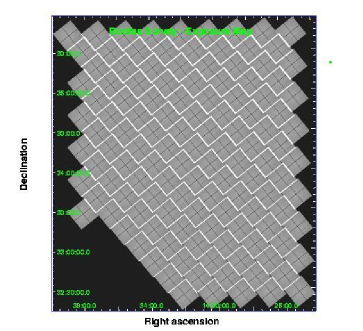
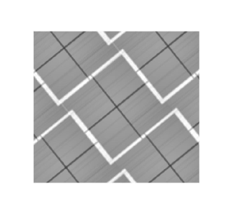
Figure 1: Left: Exposure map for Boötes Survey. There are 126 ACIS-I fields, which overlap by less than 1 arc minute (the brighter regions). Right: Expanded view near center. Due to telescope vignetting, the center of each ACIS-I field has slightly (20%) higher exposure than the edge. The lower (darker) exposure region inside each ACIS-I field is due to the gaps between the CCD chips. However, because the observatory is dithered during an observation, the exposure in the CCD gaps is not zero, but is about 50% of the average exposure.

Table 1: Boötes X-ray Observation Properties

Chandra OBSIDs	Type	Date	Locations
3596 - 3660	GTO	March 2003	Northern
4218 - 4272	GO	April 2003	Southern
4277 - 4282	GO	April 2003	Southern

In Section 2.1 we discuss the reduction procedures for the images, and in Section 2.2 we discuss the source detection procedures. Our procedures are very similar to those used by Kenter and Murray (2003) in their analysis of a smaller survey in the Lockman Hole area. Each ACIS-I field was analyzed independently and the final source lists are combined.

2.1 Data Preparation

The standard Chandra pipeline products are used with added processing as follows. First the data are checked for periods of high background or background flares following the CXC data preparation thread. During these observations we had no major background flares, and after screening, most of the individual observations have very much the same exposure time. Almost all of the fields (110 out of 126) have the same exposure time within 100 seconds, although the full range is from 4250 to 5050 seconds.

The data are filtered using the very faint mode background algorithm developed by Vikhlinin, which also removes afterglow events. Finally the data are filtered by energy, limiting the energy range to 0.5-7 keV (Total band). The final ACIS event files are then binned into image files, with a binning factor of 4 (i.e., 4x4 ACIS pixels equal 1 image pixel 1.968 arc seconds on a side). As noted above, these steps are performed on each survey observation individually, resulting in 126 image files used for source detection. In the Total band images, the typical background is $\sim 1.1\times 10^{-2}\,\mathrm{ct}/\mathrm{image\,pixel}$. Of the 126 fields, there are 6 where the background is about a factor of two higher than the rest. However, this higher background has a negligible effect on point source detection efficiency within about 6 arc minutes of the field center, particularly for sources with $\geq 4$ counts in the detection cell. Figure 2 shows the cumulative sky coverage for the XBoötes survey calculated as in Kenter & Murray (2003). Since the exposure times are all very similar, the overall sky coverage rises rapidly as a function of flux and exceeds 9 square degrees for a total band flux of $\geq 10^{-14}\mathrm{erg\,cm^{-2}sec^{-1}}$.

Figure 2: Plot of the sky coverage for the XBoötes survey. The plot gives the solid angle (in square degrees) as a function of the Total band (0.5-7.0 keV) flux in $\mathrm{erg\,cm^{-2}sec^{-1}}$. The nearly uniform exposure times of the 126 ACIS fields, accounts for the rapid rise in coverage at the lowest fluxes. The roll over between about 7 and 9 square degrees is due to the effects of vignetting and the growth of the Chandra point spread function (PSF) at large off-axis angles.

2.2 Source Detection

We used the CIAO3.0.2 wavelet detect process (wavdetect) with the “sigthresh” parameter set to $5\times 10^{-5}$ to detect point sources in each of the data sets. This relatively high “sigthresh” parameter value was set on the basis of simulations which showed that for the short exposure times of our survey (and therefore low background) the detection efficiency for faint sources is high and the spurious detection rate is low (see Paper II, Kenter et al. (2005) for details). Because we analyze the fields independently, we may detect the same source twice, if it lies in the overlap region (about 4% of the total area covered). We eliminate these duplications in our source list by selecting the detection which has a smaller radial distance from the aim-point (and therefore smaller point spread function).

The results from running wavdetect (including the elimination of duplicated sources and those with only one count) yields a combined list of 4642 point-like sources in the 0.5-7 keV energy band that have $\geq 2$ counts within the 90% encircled energy radius. We use this source list as a starting point for further analysis to recalculate source locations and fluxes from the original event data set. For each source we extracted a 100x100 ACIS pixel “postage stamp” at full ACIS spatial resolution (0.492 arc seconds per pixel) centered on the wavdetect position. We then recalculated the source position by iteratively centroiding the events within the 90% encircled energy region. We used a circle to approximate the encircled energy region with radius $R_{90}$ (in arc seconds) dependent on the square of the off-axis angle of the initial source position.

Once the source location was determined, we counted the number of events ($\mathrm{F_{50},\>F_{90}})$ within the 50% ($R_{50}$) and 90% ($R_{90}$) encircled energy regions. If the source had at least $\mathrm{F}_{50}\geq 5$ counts inside $\mathrm{R}_{50}$, we estimated the uncertainty in the source location as $\mathrm{C_{err}=R_{50}/(\sqrt{F_{50}}-1)}$, i.e., the 50% encircled energy radius divided by the approximate counting uncertainty. For sources with $F_{50}<5$ counts, we set the centroid uncertainty to be $\mathrm{C_{err}=R_{50}}.$ Finally, for all sources, we set a floor to the centroid uncertainty of $\mathrm{\mathrm{C}_{err}}=1.5$ arc seconds to account for systematic errors not included in the above analysis. These systematic effects include the non-circular shape of the Chandra/ACIS point spread function (PSF) for sources that are off-axis, the approximations associated with estimating the PSF size, and residual astrometric errors in transferring detector coordinates to the sky. Using the source positions obtained from the Total band (0.5-7 keV) analysis, we also compute the total number of counts within the 50% and 90% encircled energy regions in the Soft band (0.5-2 keV) and the Hard band (2-7 keV), and from these generate the source hardness ratio ($HR=(F90_{hard}-F90_{soft})/(F90_{hard}+F90_{soft})$). Using the exposure map data from the pipeline processing, we also compute the effective exposure time for each source, as well as the effective area fraction relative to being on-axis (this provides the correction for vignetting). The centroid uncertainties turn out to be fairly conservative, crudely corresponding to about a 90% confidence interval. We will be able to quantify this more accurately as we accumulate more spectroscopic identifications. It is already clear from the optical matches (see Brand et al., 2005) that the 1.5 arc second floor to $\mathrm{C}_{err}$ (especially for sources close to the optical axis) is generous.

3 The Distribution of Point Sources

The source catalog, giving source positions and X-ray properties, is presented in Paper II (Kenter et al., 2005). We note here that there were 4767 candidate sources from the CIAO wavdetect analysis. From the processing described in the previous section, we find a total of 4642 sources with greater than or equal to 2 counts in the 90% encircled energy region in the 0.5-7 keV Total energy band. We call this the XB2 catalog. A subset of this catalog with sources of 4 or more counts is denoted as the XB4 catalog and contains 3293 sources. As a result of simulations, we estimate that the XB2 catalog contains $\sim 14$% spurious sources, whereas the XB4 catalog contains less than 1% spurious sources. Here we discuss the spatial distribution of the sources (i.e., their projected sky distribution), along with a brief introduction to the optical matches and subsequent redshift survey.

The 125 candidate sources with fewer than 2 counts within $R_{90}$, which are not included in XB2, were examined individually and most (114 of 125) were found to have only one event within the 90% encircled energy region appropriate to the off-axis position. Since the wavdetect threshold was set high ($5\times 10^{-5}$), it is not surprising to have false candidate sources at the level of about 1 per ACIS-I field.

3.1 The Spatial Distribution of Sources

There have been claims in deep surveys covering much smaller areas for the detection of large scale structure in the distribution of sources (e.g., Yang et al. 2003, Giacconi et al. 2002). In contrast, the ChaMP found source distributions consistent with Poisson statistics in 62 disjoint Chandra fields (Kim et al. 2004). While our survey is not as deep, it is wide, contiguous in area, spatially uniform, performed with a single instrument setup, and contains many more sources that can be divided into spatial regions. Figure 3 shows the spatial distribution of the full set of Total band (0.5 - 7 keV) sources (XB2) on the sky, where each source is represented by a dot (regardless of flux). No obvious significant spatial structure is present.

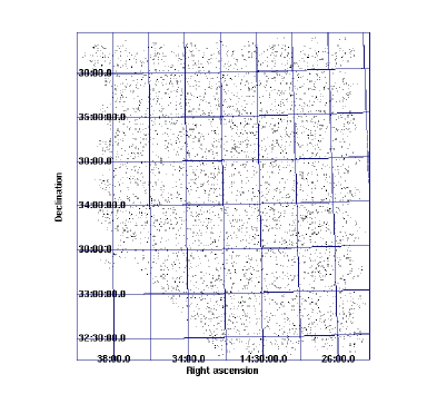
Figure 3: Locations of the 4642 sources detected in the Boötes Survey with 2 or more counts within the 90% encircled energy region of the PSF.

Figure 4 shows three different approaches to spatially smoothing the distribution of sources. On the left is a “raw image” corresponding to the number of sources in each ACIS-I field (pixels are $\sim 16$ arcminute on a side), where the color scale is darkest for the lowest number of sources. The center image is the result of Gaussian smoothing the raw image with a sigma corresponding to one ACIS-I field. There appear to be spatial correlations (i.e., large scale structures) where the source density is below the average (darker areas that run NE to SW) and above the average (brighter areas to the N and W of the dark patches). On the right we show an adaptively smoothed image from Figure 3, where the top-hat smoothing filter has an adaptive size needed to accumulate 38 counts (the average number of sources per ACIS-I field). Structures similar to those seen in the middle panel are also evident in this image. However, the significance of these structures, estimated from the net excess (or deficit) of sources compared with the average over the structure sizes, is only 2 to 2.5 sigma. The structures seen in Figure 4 are typical in appearance and magnitude to structures observed in simulations with random distributions of the same numbers of sources. We can quantify this result by examining the counts-in-cells of the 126 ACIS-I fields of view compared to the Poisson distribution for a mean of 36.84 sources per field (4642/126). As shown in Figure 5 there is no significant difference between the observed and the Poisson distributions. A $\chi^{2}$ test gives a reduced value of 0.90 for 12 degrees of freedom.

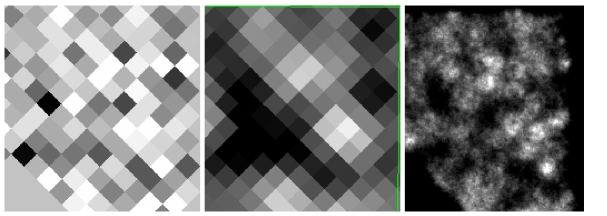
Figure 4: Spatial distribution of sources per ACIS field where lighter color means higher density. Left panel shows the “raw” data, i.e., the number of sources per ACIS-I field. The middle panel shows the same data slightly smoothed (with a Gaussian using a sigma of one ACIS FOV). The right panel is the image from Figure 3 adaptively smoothed with a 38 count threshold (the mean number of sources per field). The structures seen in the middle panel are qualitatively the same in this smoothed image.

While it would be expected that the X-ray selected AGN are good tracers of the cosmic web and large scale structure, it is not very surprising that we find no evidence for large scale structure based on this technique. Even with $\sim 4500$ sources, it would take quite large amplitude structures to overcome the statistical fluctuations after dividing the data into 126 spatial bins. At $z\sim 1$, an ACIS-I field corresponds to about $8h^{-1}$ Mpc, a scale on which the three-dimensional correlation function should have an amplitude near unity (Croom et al., 2002). In projection, however, we have averaged over the line-of-sight distance which is 450 times larger than that scale size, and hence we would expect fluctuations of only order $1/\sqrt{450}\sim 5\%$, which are too small to see against Poisson noise. Clear detections of large scale structure on these scales will require redshifts (either spectroscopic or photometric), so that the correlations will not be washed out by projection effects along the large line-of-sight. In section 3.4 we discuss some preliminary results on the redshift distribution of a sample from the XB4 catalog that were obtained from the AGN and Galaxy Evolution Survey (AGES, Kochanek et al. 2005), which (when complete) will yield accurate spectroscopic redshifts for about half of the sources in the XB4 catalog as well as some of the optically bright sources at lower flux from the XB2 catalog.

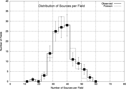
Figure 5: Distribution of sources per field in XBoötes Survey. The solid curve shows the number of fields in XBoötes as a function of the number of sources (0.5 - 7 keV band, $\geq 2$ counts) detected in that field. The dashed curve is the expected Poisson distribution for the mean number of sources per field 36.84) and the number of fields (126).

3.2 Large Scale Structure and Angular Correlation

Statistical evidence of large scale structure (LSS) in X-ray surveys has been reported by Vikhlinin & Forman (1995), Giacconi et al. (2001), Yang et al. (2003) and others. Previous X-ray surveys looking for LSS typically have been limited to narrow field or disjoint serendipitous surveys with spatially varying levels of sensitivity. The ROSAT survey has further been subject to systematic errors and biases, due to poor angular resolution (Vikhlinin & Forman 1995.) These Chandra XBoötes data are unique in that they constitute the widest (9.3 deg²), contiguous X-ray field yet observed to such a faint flux limit as $4\times 1\mathrm{0^{-15}erg\,cm^{-2}\,s^{-1}}$. The angular resolution, uniform coverage and large contiguous field of view allow us to search for evidence of structure on both small and large angular scales, relatively free of edge effects and position inaccuracy biases.

In the absence of redshift information, we used the Landy and Szalay (1993) estimator to determine the angular correlation function of the X-ray sources. The random catalogs required for the estimate were generated by drawing sources from the CDS logN-logS distribution (Giacconi et al. 2001), and using the MARX (Wise et al. 1997) simulator for the response of the Chandra X-ray Observatory. MARX simulates telescope, detector and observatory features such as quantum efficiency, inter-CCD chip gaps, vignetting, PSF and spacecraft dither. We have verified that our Monte Carlo simulations reproduce many features present in the real data, such as the fall off in detection sensitivity with off axis angle.

In total, we simulated the entire XBoötes field sixteen times, detecting $42,000$ simulated sources. The simulations reflect all biases and features of the real XB2 data set. Taking into account the integral constraint (Groth & Peebles 1977, Efstathiou et al. 1991), we find a positive angular correlation in the full XB2 source catalog on scales of $\geq 1$ arcminute, as shown in Figure 6. The error bars shown are based on Poisson statistics ($\Delta\omega=[\omega(\theta)+1]/\sqrt{DD}$ c.f., Wall & Jenkins (2003)). The results for $\theta\geq 1$ arc-minute are consistent with those previously given by Vikhlinin & Forman (1995), who reported a correlation described by the power law, $\omega(\theta)=(\frac{\theta}{\theta_{0}})^{-0.7}$ with $\theta_{0}\sim 4$ arcseconds. On smaller scales the number of source pairs in our data set is small and we have only upper limits. However, we have plotted the correlation results from Giacconi et al. (2001) (their Figure 6) which extend to small angles and are consistent with our results. Also plotted is the somewhat steeper power law that Giacconi et al. (2001) show in their figure. Our results are fully consistent with these previous correlations.

Figure 6: The angular correlation function $\omega(\theta)$ for the XBoötes Survey (filled squares and solid lines) derived using the Landy and Szalay statistic $\omega(\theta)=(DD-2DR+RR)/RR$ and correcting for the integral constraint. We find a positive angular correlation on scales of $\geq 1$ arcminute. These results are consistent with the power law curve (shown as the heavy dotted line with index -0.7 and $\theta_{0}=4$ arcseconds) of Vikhlinin & Forman (1995) and a similar power law (shown as the light dotted line with index -1.0 and $\theta_{0}=10$ arcseconds) of Giacconi et al. (2001). Also plotted, as the open squares and dashed lines, are the results from Giacconi et al. (2001) (their Figure 6), which are consistent with our results and the power law curves shown.

3.3 Optical Counterparts from the NDWFS

The XBoötes X-ray survey field was chosen the cover the same region as the Boötes field of the NOAO Deep Wide-Field Survey: a deep optical and near-IR imaging survey designed to study the formation and evolution of large scale structure (Jannuzi & Dey 1999). In this section, we present preliminary results on the identification of the optical $(B_{W},\,R,\,I)$ and near-IR $(K)$ counterparts to the XB4 catalog in a $1.4\,\mathrm{deg^{2}}$ sub-region of the full Boötes area. There are 481 X-ray sources in the sub-region of which we expect less than 1% to be spurious (Kenter et al. 2005). We find an optical counterpart for 87% of the XB4 X-ray sources. We assign an X-ray source to have an optical counterpart if there is at least one optical source with a detection in at least one optical band in the region enclosed by the X-ray positional errors ($\mathrm{C_{err}}$; Section 2.2). The NDWFS positions have small astronomical uncertainties (typically $0.1-0.4$ arcseconds, RMS) that can be considered negligible in comparison to the positional error of the X-ray sources (Section 2.2). Figure 7 shows the cumulative fraction of matches brighter than a given magnitude in the $B_{W},\,R,\,I$ and $K$ bands. The $K$-band catalog is not as deep as the optical catalogs and therefore does not match the depth of XBoötes, resulting in a smaller fraction of matches. In Brand et al. (2005), we present a more sophisticated Bayesian identification scheme which self-consistently evaluates the probability of each of the optical sources surrounding an X-ray source being more probable than a ’background’ source. We also present the matched X-ray / optical catalog for the entire survey area.

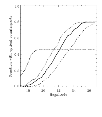
Figure 7: The cumulative fraction of X-ray sources with optical counterparts brighter than a given magnitude (Vega) in the $R$-band (solid line), $B_{W}$-band (dashed line), $I$-band (dotted line) and $K$-band (dot-dashed line), taken from Brand et al. (2005)

3.4 Optical Spectroscopy

The AGN and Galaxy Evolution Survey (AGES, Kochanek et al. 2005) targeted all of the XB4 sources matched to an optical source brighter than R=21.5 mag. Fainter X-ray sources from the XB2 catalog were targeted if there were otherwise unallocated fibers. Spectra were obtained with the MMT using the 300-fiber Hectospec robotic spectrograph (Fabricant et al., 1998) in Spring and Summer of 2004. We (Kochanek et al., 2005) obtained optical spectra for 1231 X-ray selected targets, and the preliminary reduction of these spectra have resulted in 892 well-determined redshifts and preliminary spectral classifications for these sources. While more work is yet to be done, we find that, as expected, the detection of X-rays preferentially identifies AGN from the “sea” of galaxies in the NDWFS, and that at the sensitivity level reached in this survey, most of the AGN are at a redshift of about 1. Of the 892 X-ray objects with preliminary redshifts, 25 are stars, 249 are classified as galaxies, 43 are classified Sy 1/2 galaxies, and 575 classified as QSO/Sy 1 galaxies. These classifications are based on template matching of the extracted spectra (about 6 FWHM resolution) using either a galaxy template (i.e., absorption lines) or an emission line template. The AGN/Sy 1 have broad lines and the Sy 1/2 have either [NeV] 3426 at ¿ 2.5$\sigma$, or [N II] ¿ H$\alpha$, [OI] 6300 exists and [O III] 5007 $>2\times\mathrm{H}\beta$. It is possible that some of the objects classified as galaxies have lower significance AGN emission lines which were not flagged by this analysis.

The redshift distributions for galaxies (not flagged as any kind of AGN), and AGN (QSO/Sy 1/Sy 2) are shown on the left panel of Figure 8. Treister et al. (2004) and Barger et al. (2005) plot redshift distributions for the AGN found in the Chandra Deep Fields showing peaks near z=1. Barger et al. (2005) give the median redshift as a function of X-ray flux, and for the flux range of the XBoötes survey, these are all near z=1. The peak for the XBoötes AGN is also peaked around z=1 consistent with these results. With only a preliminary separation of galaxy and AGN classes, it is not appropriate to compare our redshift distribution in detail with those for CDFS (e.g., Szokoly et al., 2004) or detailed models such as those of Treister et al. (2004). The long tail out to redshifts as high as 3.9 is not surprising, as the survey area is large enough to find rare very high luminosity AGN at large redshift.

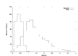
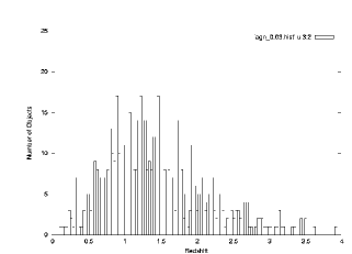
Figure 8: Redshift distributions. Left: for galaxies (dashed) and AGN (solid) from AGES measurements using the MMT/Hectospec.. Right: More finely binned (0.03) for AGN only showing possible spikes that might correspond to large scale structure features.

The right panel of Figure 8 shows the distribution of AGN with a finer binning (0.03 in z). There are several spikes in the distribution which, if real, would indicate the presence of large scale structure. We have used a one-sided statistical test of Nulsen and Murray (2005, in preparaton) to search for significant excesses in the redshift bins. Given the spareness of the data available, we do not consider any of the spikes in our current redshift distribution to be firm evidence for large scale structure. However, once all of the X-ray selected AGN have been observed as part of our ongoing AGES program, there should be about twice the number of objects and therefore sufficient statistics to identify redshift concentrations corresponding to actual large scale structures.

The quality of the AGES spectra are illustrated in Figure 9 where we show the optical finding chart and preliminary spectrum for one of the highest redshift sources, CXOXB J142547.4+352719 (aka NDWFS J142547.4+352719), a quasar at z=3.53 which has 12 counts in the Total band (0.5-7 keV), corresponding to a luminosity $\mathrm{L_{x}}=2.8\times 10^{45}\mathrm{\,erg\,cm^{-2}s^{-1}}$ (using $\lambda\mathrm{CDM}$ with $H_{0}=71,\>\Omega_{m}=0.27,\>\mathrm{and}\>\Omega_{\lambda}=0.73$).

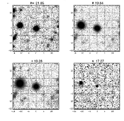
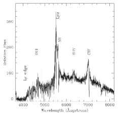
Figure 9: Finding chart for NDWFS J142547.4+352719 (aka CXOXB J142547.4+352719), a z=3.53 AGN and its preliminary spectrum.

4 Conclusions

We have conducted a large area survey using 126 Chandra ACIS-I pointings to cover 9.3 square degrees of the NDWFS in Boötes. We find no evidence for major deviations from a uniform sky density of sources at the flux levels reached in $\sim 5000$ seconds of Chandra observing time, but there is some hint of spatial structure on a scale of several Mpc which may be due to the X-ray selected AGN population tracing out large scale structures. The two-point angular correlation for $\theta\geq 1$ arcminute does show the same power law correlation as noted previously (e.g., Vikhlinin & Forman 1995, Giacconi et al. 2001).

The X-ray survey and the NDWFS are well matched as evidenced by the high (87%) success rate (Brand et al. 2005) of associating X-ray sources with optical candidates. Follow up optical spectroscopy as part of AGES (Kochanek et al. 2005) has yielded good classification and redshift results, with 892 preliminary redshifts out of 1231 targets, most of which were brighter than R=21.5. There are hints in the binned redshift distribution of these X-ray selected AGN for excesses at several redshifts. However, the small number of objects per redshift bin does not allow for these to be taken as firm evidence for large scale structures. These initial redshifts, plus additional spectroscopic redshifts expected from future AGES observations (and ultimately augmented with a comparable number of photometric redshifts) will permit a statistically interesting view of the spatial distribution of the X-ray selected sources and their relationship to large scale structures as traced by the galaxy spectroscopy.

5 Acknowledgements

This work was supported through the Smithsonian Institution and by NASA Contracts NAS8-38248, NAS8-01130, NAS8-39073, NAS8-03060, and NASA Grant GO3-4176A. This work was also supported by the National Optical Astronomy Observatory which is operated by AURA, Inc, under a cooperative agreement with the National Science Foundation. We appreciate the excellent support we have received from the CXC Mission Planners in carrying out these observations, the CXC Data Processing Team for the pipeline data, the NDWFS Team for the optical observations and data reduction, and the AGES Team in obtaining reduced spectra. We would like to thank the anonymous referee for helpful suggestions that improved this paper.

References

- Barger et al. (2005) Barger, A. J., Cowie, L. L., Mushotzky, R. F., Yang, Y., Wang, W.-H., Steffen, A. T., & Capak, P. 2005, AJ, 129, 578
- Becker et al. (1996) Becker, R. H., Gregg, M. D., Helfand, D. J., & et al., 1996, in IAU Symp. 175: Extragalactic Radio Sources, 499–+
- Brand et al. (2005) Brand, K., et al. 2005, ApJ (submitted)
- Brandt et al. (2001) Brandt, W. N., et al. 2001, AJ, 122, 2810
- Casertano et al. (2000) Casertano, S., et al. 2000, AJ, 120, 2747
- Chatzichristou (2004) Chatzichristou, E. T. 2004, Advances in Space Research, 34, 661
- Colless et al. (2001) Colless, M., et al. 2001, MNRAS, 328, 1039
- Cress et al. (1996) Cress, C. M., Helfand, D. J., Becker, R. H., Gregg, M. D., & White, R. L. 1996, ApJ, 473, 7
- Croom et al. (2002) Croom, S. M., Boyle, B. J., Loaring, N. S., Miller, L., Outram, P. J., Shanks, T., & Smith, R. J. 2002, MNRAS, 335, 459
- de Vries et al. (2002) de Vries, W. H., Morganti, R., Röttgering, H. J. A., Vermeulen, R., van Breugel, W., Rengelink, R., & Jarvis, M. J. 2002, AJ, 123, 1784
- Efstathiou et al. (1991) Efstathiou, G., Bernstein, G., Tyson, J. A., Katz, N., & Guhathakurta, P. 1991, ApJ, 380, L47
- Eisenhardt et al. (2004) Eisenhardt, P. R., et al. 2004, ApJS, 154, 48
- Fabricant et al. (1998) Fabricant, D. G., Hertz, E. N., Szentgyorgyi, A. H., Fata, R. G., Roll, J. B., & Zajac, J. M. 1998, in Proc. SPIE Vol. 3355, p. 285-296, Optical Astronomical Instrumentation, Sandro D’Odorico; Ed., 285–296
- Giacconi et al. (2001) Giacconi, R., et al. 2001, ApJ, 551, 624
- Giacconi et al. (2002) Giacconi, R., et al. 2002, ApJ Suppl, 139, 369
- Green et al. (2004) Green, P. J., et al. 2004, ApJS, 150, 43
- Groth & Peebles (1977) Groth, E. J. & Peebles, P. J. E. 1977, ApJ, 217, 385
- Jannuzi & Dey (1999) Jannuzi, B. T. & Dey, A. 1999, in ASP Conf. Ser. 191: Photometric Redshifts and the Detection of High Redshift Galaxies, ed. L. Weymann, L. Storrie-Lombardi, M. Sawicki, & R. Brunner, 111–+
- Kenter et al. (2005) Kenter, A. et al. 2005, ApJ (submitted)
- Kenter & Murray (2003) Kenter, A. T. & Murray, S. S. 2003, ApJ, 584, 1016
- Kim et al. (2004) Kim, D.-W., et al. 2004, ApJ, 600, 59
- Kochanek et al. (2005) Kochanek, C. et al. 2005, ApJ (in preparation)
- Martin et al. (2003) Martin, C., et al. 2003, in Future EUV/UV and Visible Space Astrophysics Missions and Instrumentation. Edited by J. Chris Blades, Oswald H. W. Siegmund. Proceedings of the SPIE, Volume 4854, pp. 336-350 (2003)., 336–350
- Soifer & Spitzer/NOAO Team (2004) Soifer, B. T. & Spitzer/NOAO Team. 2004, American Astronomical Society Meeting, 204,
- Szokoly et al. (2004) Szokoly, G. P., et al. 2004, ApJS, 2004, 155, 271
- Treister et al. (2004) Treister, E., et al 2004, ApJ, 616, 123
- Vikhlinin & Forman (1995) Vikhlinin, A. & Forman, W. 1995, ApJL, 455, L109+
- Wall & Jenkins (2003) Wall, J. V. & Jenkins, C. R. 2003, Practical statistics for astronomers (Princeton Series in Astrophysics)
- Williams et al. (1996) Williams, et al. 1996, AJ, 112, 1335
- Wise et al. (1997) Wise, M. W., Huenemoerder, D. P., & Davis, J. E. 1997, in ASP Conf. Ser. 125: Astronomical Data Analysis Software and Systems VI, 477–+
- Yang et al. (2003) Yang, Y., Mushotzky, R. F., Barger, A. J., Cowie, L. L., Sanders, D. B., & Steffen, A. T. 2003, ApJ, 585, L85
- York et al. (2000) York, D. G., et al. 2000, AJ, 120, 1579