$J$-resolved He I emission predictions in the low-density limit

Abstract

Determinations of the primordial helium abundance are used in precision cosmological tests. These require highly accurate He I recombination rate coefficients. Here we reconsider the formation of He I recombination lines in the low-density limit. This is the simplest case and it forms the basis for the more complex situation where collisions are important. The formation of a recombination line is a two-step process, beginning with the capture of a continuum electron into a bound state and followed by radiative cascade to ground. The rate coefficient for capture from the continuum is obtained from photoionization cross sections and detailed balancing, while radiative transition probabilities determine the cascades. We have made every effort to use today’s best atomic data. Radiative decay rates are from Drake’s variational calculations, which include QED, fine structure, and singlet-triplet mixing. Certain high-$L$ fine-structure levels do not have a singlet-triplet distinction and the singlets and triplets are free to mix in dipole-allowed radiative decays. We use quantum defect or hydrogenic approximations to include levels higher than those treated in the variational calculations. Photoionization cross sections come from $R$-matrix calculations where possible. We use Seaton’s method to extrapolate along sequences of transition probabilities to obtain threshold photoionization cross sections for some levels. For higher $n$ we use scaled hydrogenic theory or an extension of quantum defect theory. We create two independent numerical implementations to insure that the complex bookkeeping is correct. The two codes use different (reasonable) approximations to span the gap between lower levels, having accurate data, and high levels, where scaled hydrogenic theory is appropriate. We also use different (reasonable) methods to account for recombinations above the highest levels individually considered. We compare these independent predictions to estimate the uncertainties introduced by the various approximations. Singlet-triplet mixing has little effect on the observed spectrum. While intensities of lines within multiplets change, the entire multiplet, the quantity normally observed, does not. The lack of high-precision photoionization cross sections at intermediate-$n$, low-$L$ introduces $\sim 0.5\%$ uncertainties in intensities of some lines. The high-$n$ unmodeled levels introduce $\sim 1\%$ uncertainties for yrast lines, those having $L=n-1$ upper levels. This last uncertainty will not be present in actual nebulae since such high levels are held in statistical equilibrium by collisional processes. We identify those lines which are least affected by uncertainties in the atomic physics and so should be used in precision helium abundance determinations.

1 Introduction

The spectra of hydrogen and helium emitted in the recombination process $A^{+}+e^{-}\to A^{\ast}+\,\hbar\omega$ followed by subsequent cascades $A^{*}\to A^{\prime*}+\hbar\omega^{\prime}$, have long played a fundamental role in studies of cosmic chemical evolution. The relative intensities of the emission lines depend mainly on the abundances of $\mbox{H}^{+}$ and $\mbox{He}^{+}$, not on uncertain plasma conditions such as temperature and density, so ionic abundances can be determined with a precision that is limited instead by measurement errors and atomic theory. Much effort has gone into precision measurements of He/H abundance ratios with a particular emphasis on using the primordial abundance of He as a test of the Big Bang (Pagel, 1997, hereafter P97). This requires that theoretical emission spectra be understood to a precision better than $1\%$.

Calculation of the hydrogen recombination-cascade spectrum was one of the first applications of quantum mechanics to astrophysics (Baker & Menzel, 1938, hereafter BM38). Hydrogen is a simple system, and it is thought that current predictions Storey & Hummer (1995) are accurate to substantially better than $1\%$. The atomic physics of helium, being a two-electron system, is more complex. It was only much later that its recombination-cascade spectrum was first computed (see Brocklehurst 1972 for discussion), and recent studies have been published by Smits (1991,1996) and Benjamin et al. (1999, hereafter BSS99). Each succeeding study improved the prior treatment of physical processes, mainly as the result of improved theoretical calculations of various rates. But the bookkeeping associated with solving the numerical problem involving several hundreds or thousands of levels is also intricate, and mistakes are almost unavoidable. Many of the successive papers found numerical errors in the preceding work.

This paper revisits the He I recombination-cascade spectrum in the low-density limit. We make the following improvements. $\mbox{He}^{0}$ has previously been modeled as distinct singlet and triplet systems with $n\,{}^{2S+1}\!L$ terms. The present calculation utilizes fine-structure $n\,{}^{2S+1}\!L_{J}$ levels. In $L\geq 3$ levels, however, the spin-orbit interaction leads to strong singlet-triplet mixing. We use Drake’s (1996, hereafter D96) highly accurate calculations of the $J$-resolved transition probabilities, which take this singlet-triplet mixing into account. We carry out the calculation with $J$-resolved transitions twice: once with singlet-triplet mixing explicitly included ($ST$-mixing) and once with $LS$-coupling assumed ($LS$-coupling). Comparison of emission line intensities (or emission coefficients) allows us to ascertain directly the effects of including singlet-triplet mixing. Finally, to avoid bookkeeping errors, we do calculations with two independently developed codes to confirm predictions. The second code Porter et al. (2005) assumes pure $LS$-coupling and is not a $J$-resolved calculation. By summing the emissions from the $J$-resolved levels, we can compare the emission coefficients to other multiplet-emission calculations.

Based on the principle of spectroscopic stability (Condon & Shortley 1991), only small changes are to be expected in multiplet-average line intensities, either as a result of allowance for $J$-splittings within $LS$-coupled terms or mixing between singlets and triplets. This is because both of these effects can be expressed, at least to lowest order, in terms of unitary transformations of the zero-order states, and the difference between the sum-of-squares of electric-dipole matrix elements and the calculation of multiplet emission or absorption strength hinges only on the tiny energy splittings involved. By the same token, however, multiplet-average emission or absorption cannot be exactly independent of the allowance for fine-structure and singlet-triplet mixing because of these very splittings, and without explicit calculation the deviations, which are potentially important for accurate interpretation astrophysical data, cannot be guessed.

Although extremely accurate atomic data now exist for the lower levels $\mbox{He}^{0}$, we find that they do not extend to a high enough $n$ for the lower non-hydrogenic $L$ that are needed for definitive predictions of the spectrum. Various assumptions are made to bridge the gaps between states with precise atomic data and those for high $n$ and low $L$. We identify the atomic data that introduce the greatest uncertainty in the final spectrum. Section 2 discusses the necessary atomic physics and data sources. Section 3 describes the formation and solutions of the recombination-cascade problem. The results of this study are presented in Section 4, and conclusions are stated in Section 5.

2 Atomic Data

The accuracy of the recombination and radiative cascade model presented here is determined mainly by the atomic data. A description of the relevant quantities, techniques, and references is given below. The high-precision calculations of D96 are used extensively in the calculation of level energies, quantum defects, oscillator strengths, and matrix elements for $n\leq 10$. Extrapolations of the D96 results are used in the calculation of some atomic data for the higher lying levels.

Here we are only interested in transitions between pairs of singly excited levels in helium sharing a $1s$ core configuration. For these levels the total orbital angular momentum $L$ equals the orbital angular momentum of the excited electron $\ell$. We will use the notation $\gamma_{u}\equiv\{n_{u},L_{u},S_{u},J_{u}\}$ for the initial (upper) level of an emission line and similarly $\gamma_{l}\equiv\{n_{l},L_{l},S_{l},J_{l}\}$ for the final (lower) level and $\gamma\equiv\{n,L,S,J\}$ for a level in general. We designate continuum levels with free electron energy $\varepsilon$ as $\gamma(\varepsilon)\equiv\{\varepsilon,L,S,J\}$.

2.1 Level Energies

We calculate the level energies in helium, depending on $n$ and $L$, by three methods. For levels $n\leq 10$ and $L\leq 7$, ionization energies $E$ are obtained from the Rayleigh-Ritz variational relativistic calculations of D96. For all levels $L\geq 8$, the asymptotic multipole expansion method Drake 1993a ; Drachman (1993) is used to calculate the (negative) eigenenergies $E_{0}$. Ionization energies are found from the relation $E=(-E_{0}-4\,hcR_{\mathrm{He}^{2+}})$ where $R_{\mathrm{He}^{2+}}$ is the Rydberg constant for an electron-plus-alpha-particle system. For levels $n\geq 10$ and $L\leq 7$, ionization energies are found from the Ritz quantum defect expansion (D96). These energies include all relativistic and quantum electrodynamic (QED) corrections to the nonrelativistic eigenenergies through order $\alpha^{4}_{\mathrm{fs}}$, where $\alpha_{\mathrm{fs}}$ is the fine-structure constant. Overlap at the boundaries of the three $nL$ regions allows us to verify the accuracy of our implementation.

For each $n$ and $L$, the energies of the two levels with $J=L$ (e.g. $n\,{}^{3}\!L_{L}$ and $n\,{}^{1}\!L_{L}$) are shifted by the off-diagonal fine-structure ($J$-resolved) matrix elements connecting these two levels (MacAdam & Wing, 1978, hereafter MW78) to give the singlet-triplet mixing energies. Quantum defects $\delta$ and effective quantum numbers $\nu=n-\delta$ are then calculated from the modified level energies.

Exact analytical solutions to the nonrelativistic Schrödinger equation are known for two-body systems ($e.g.$ atomic hydrogen). For helium, approximate solutions based on the Rayleigh-Ritz variational principle are now available (D96) and are essentially exact. Relativistic and QED corrections are then added, including both diagonal and off-diagonal matrix elements of spin-orbit and spin-other-orbit interactions (D96, Drake 1993b). It is these off-diagonal matrix elements that mix levels of different total spin $S$ and are responsible for the breakdown of $LS$-coupling.

For all levels with $L\geq 8$, the asymptotic expansion describes the interaction of the Rydberg electron with the $\mbox{He}^{+}$ core in terms of core-polarization multipole moments Drachman (1993). This approximation agrees with the full variational calculation at $L=7$ and further improves with increasing $L$.

The ionization energies of excited helium Rydberg levels deviate from hydrogenic values and may be represented by

$$E(\gamma)=\frac{hcR_{\mathrm{He}^{+}}}{(n-\delta(\nu))^{2}}\,$$ (1)

$R_{\mathrm{He}^{+}}$ is the Rydberg constant for the reduced mass of the electron-$\mbox{He}^{+}$ system. The quantum defects $\delta(\nu)$, in addition to having a dependence on $S$, $L$, and $J$, also depend weakly on $\nu$. $\nu$ is found by an iterative solution to the equation, $\nu=n-\delta(\nu)$, where in the Ritz expansion (Edlén 1964)

$$\delta(\nu)=\delta_{0}+\frac{\delta_{2}}{(n-\delta(\nu))^{2}}+\frac{\delta_{4}}{(n-\delta(\nu))^{4}}+\cdots$$ (2)

The constant coefficients $\delta_{i}$ used here are given by D96.

2.2 Bound-bound transitions

The emission oscillator strength $f_{ul}$ (dimensionless) and the spontaneous radiative transition rate coefficient (Einstein $A$; s^-1) are principal atomic quantities related to line strengths for transitions between an initial upper level $\gamma_{u}$ and a final lower level $\gamma_{l}$. The Einstein $A$ coefficients are the most convenient quantity for calculating the elements of the cascade matrix while theoretical atomic work usually refers to oscillator strengths. The relationship between the two for the electric dipole transitions in SI units is:

$$A_{ul}=\frac{2\pi e^{2}}{m_{e}c\varepsilon_{o}\lambda^{2}}f_{ul},$$ (3)

where $\lambda$ is the vacuum wavelength.

2.2.1 Drake’s emission oscillator strengths

For transitions with $\Delta S=0$, $n_{l}\leq n_{u}\leq 10$, and both $L_{u}$ and $L_{l}\leq 7$, including those with $\Delta n=0$, the tabulated emission oscillator strengths of D96 are used. These are high precision $J$-resolved calculated values which include QED, relativistic fine-structure and non-fine-structure corrections. The largest relativistic correction comes from singlet-triplet mixing between levels with the same $n$, $L$, and $J$. In addition,  D96 provides oscillator strengths and Einstein $A$ coefficients both assuming pure $LS$-coupling (i.e. no singlet-triplet mixing) and with singlet-triplet mixing included. Emission oscillator strengths for transitions with $f_{ul}\leq 10^{-6}$ are omitted, but we calculate them by a Coulomb approximation method described later.

2.2.2 Extrapolated emission oscillator strengths

For transitions with $\Delta S=0$, and $n_{u}\geq 11$ and $n_{l}\leq 7$ and either $L_{u}\leq 6$ or $L_{l}\leq 6$, the emission oscillator strengths are derived by extrapolating those of D96. To find the emission oscillator strength $f_{ul}$ we extrapolate the series $f_{jl}$ with $\gamma_{j}\equiv\{n_{j},S_{u},L_{u},J_{u}\}$ for $n_{j}=n_{l}+1,n_{l}+2,\cdots,10$. This series is fitted as $\ln(\nu_{j}^{3}\,f_{jl})=a+bx+cx^{2}$, with $x=\ln(E_{l}/E_{jl})$, as suggested by Hummer & Storey (1998, hereafter HS98). The oscillator strength dependency for large $n$, $f\sim\nu^{-3}$, is represented by the $\nu_{j}^{3}$ factor. Parameters $a,b,$ and $c$ are determined by the fit. Here $E_{l}$ is the ionization energy of level $\gamma_{l}$ and $E_{jl}$ is the energy difference between levels $\gamma_{j}$ and $\gamma_{l}$. For some series with small $n_{j}$, the lowest lying members are omitted from the fit to obtain a better estimate of the parameters.

2.2.3 Coulomb approximation method

A Coulomb approximation method (van Regemorter, 1979, hereafter R79) is used to calculate the oscillator strengths for all remaining transitions except for those with $L_{u}=n_{u}-1$ or $L_{l}=n_{l}-1$. In transitions involving ${}^{1}P$ levels, the method is extended to account for negative quantum defects, a special case not addressed in R79. Emission oscillator strengths for weak transitions not included in D96 are calculated using this method. This simple method is particularly suitable for transitions involving high Rydberg levels with $\nu_{l},\nu_{u}>20$ and $\Delta\nu\ll\nu_{l},\nu_{u}$ where $\Delta\nu=\nu_{u}-\nu_{l}$. It agrees with the Bates & Damgaard (1949) results for $\nu_{l},\nu_{u}<20$ and with hydrogenic results for which $\nu$ takes an integer value. The method is based on the observation that, for fixed values of $\Delta\nu$, $L_{u}$, and $L_{l}$, the variation of the radial integrals $R_{\gamma_{l}}^{\gamma_{u}}$ with $\nu_{u}$ (or $\nu_{l}$) is very slow. Therefore, one of the principal quantum numbers may be taken to be an integer, and the results may be obtained accurately by interpolation.

2.2.4 Hydrogenic oscillator strengths

The remaining oscillator strengths are all taken to be hydrogenic. The emission oscillator strengths are hydrogenic if quantum defects of the upper and lower levels are nearly zero. The radial integrals $R_{\gamma_{l}}^{\gamma_{u}}$ necessary to find the oscillator strengths for these transitions are calculated by the hydrogenic solution of Hoang-Bing (1990, hereafter HB90), which is an accurate and efficient method to calculate the exact analytical solution of Gordon (1929).

2.2.5 $J$-resolved oscillator strengths

The methods of R79 or HB90 provide radial integrals and are used to calculate the $J$-resolved emission oscillator strengths. The (mean) oscillator strength is defined by

$$f_{ul}=\delta_{S_{u}S_{l}}\frac{2\mu\omega}{3\hbar}\sum\limits_{M_{l}=-J_{l}}^{J_{l}}{\frac{1}{2J_{u}+1}\sum\limits_{M_{u}=-J_{u}}^{J_{u}}{|\langle}}\,\gamma_{u}\;M_{u}|\mathord{\buildrel\lower 3.0pt\hbox{$\scriptscriptstyle\rightharpoonup$}\over{r}}|\gamma_{l}\;M_{l}\rangle|^{2}.$$ (4)

Here $\omega=(E_{u}-E_{l})/\hbar$ is the transition frequency, $\mu$ is the reduced mass, and $\delta$ is the Kronecker delta. When the angular momentum operators $L$ and $S$ that sum to $J$ are decoupled, the oscillator strength may be written

$$f_{ul}=\delta_{S_{u}S_{l}}\frac{2\mu\omega}{3\hbar}\frac{(2J_{l}+1)\,L_{>}}{(2L_{u}+1)}\left\{\matrix{{L_{u}}&{1}&{L_{l}}\cr{J_{l}}&{S_{u}}&{J_{u}}\cr}\right\}^{2}\,\left({\int\limits_{0}^{\infty}{dr\;\phi^{\ast}(\gamma_{u};r)\;r\;\phi(\gamma_{l};r)}}\right)^{2}.$$ (5)

Here $L_{>}=\mathrm{max}(L_{u},L_{l})$ and the {} factor is a Wigner 6$j$ symbol (see Edmunds 1960). The expression in parentheses is the radial integral $R_{\gamma_{l}}^{\gamma_{u}}$ discussed earlier. The function $\phi(\gamma_{l};r)$ is the radial part of the wavefunction $\Psi(\gamma;\vec{r})=r^{-1}\,\phi(\gamma;r)\,Y^{M_{L}}_{L}(\Omega)$. Oscillator strengths for $\Delta S\neq 0$ (allowed by singlet-triplet mixing) are discussed in the following subsection.

2.2.6 Oscillator strengths under singlet-triplet mixing

The largest relativistic correction to helium oscillator strengths comes from singlet-triplet mixing. This occurs most significantly between the two nominally singlet and triplet $LS$-coupled components with $J=L$ of a given $nL$ (e.g. $4\,{}^{3}D_{2}$ and $4\,{}^{1}D_{2}$). The largest component to the correction is due to the magnetic inner-spin outer-orbit interaction. The $P$ and $D$ series are only very weakly mixed, because the singlet-triplet basis states are widely separated by the electron exchange interaction. Substantial mixing occurs in $F$ levels, where exchange is much weaker, and for $L\geq 4$ the two $J=L$ energy eigenstates in each $nL$ multiplet are almost equal mixtures of singlet and triplet character. Oscillator strengths are obtained from the rediagonalization of the $(2\times 2)$ matrices for these pairs of levels as described by the mixing angle $\theta$ (D96). The mixed-spin wave functions $\Psi$ obtained by rediagonalization from the unmixed wavefunctions $\Psi_{0}$ are

$$\begin{array}[]{l}\Psi(n\,{}^{1}L_{L})=+\Psi_{0}(n\,{}^{1}L_{L})\cos\theta+\Psi_{0}(n\,{}^{3}L_{L})\sin\theta\\ \Psi(n\,{}^{3}L_{L})=-\Psi_{0}(n\,{}^{1}L_{L})\sin\theta+\Psi_{0}(n\,{}^{3}L_{L})\cos\theta.\\ \end{array}$$ (6)

We retain the traditional notation for the mixed-spin wavefunctions with the understanding that only in the limit $\theta\rightarrow 0$ are the indicated multiplicities exact. The corresponding corrected (singlet-triplet mixed) oscillator strengths $\tilde{f}_{\gamma{\gamma}^{\prime}}$ for the singlet ($s$) and triplet ($t$) components of a $\gamma\to{\gamma}^{\prime}$ transition are written in terms of the unmixed oscillator strengths $f_{\gamma{\gamma}^{\prime}}$ as

$${\begin{array}[]{*{20}c}\tilde{f}_{\gamma{\gamma}^{\prime}}^{ss}=\omega_{\gamma{\gamma}^{\prime}}^{ss}(X_{\gamma{\gamma}^{\prime}}^{ss}\cos\theta_{\gamma}\cos\theta_{\gamma}^{\prime}+X_{\gamma{\gamma}^{\prime}}^{tt}\sin\theta_{\gamma}\sin\theta_{\gamma}^{\prime})^{2}\hfill\\ \tilde{f}_{\gamma{\gamma}^{\prime}}^{tt}=\omega_{\gamma{\gamma}^{\prime}}^{tt}(X_{\gamma{\gamma}^{\prime}}^{ss}\sin\theta_{\gamma}\sin\theta_{\gamma}^{\prime}+X_{\gamma{\gamma}^{\prime}}^{tt}\cos\theta_{\gamma}\cos\theta_{\gamma}^{\prime})^{2}\hfill\\ \tilde{f}_{\gamma{\gamma}^{\prime}}^{st}=\omega_{\gamma{\gamma}^{\prime}}^{st}(X_{\gamma{\gamma}^{\prime}}^{ss}\cos\theta_{\gamma}\sin\theta_{\gamma}^{\prime}-X_{\gamma{\gamma}^{\prime}}^{tt}\sin\theta_{\gamma}\cos\theta_{\gamma}^{\prime})^{2}\hfill\\ \tilde{f}_{\gamma{\gamma}^{\prime}}^{ts}=\omega_{\gamma{\gamma}^{\prime}}^{ts}(X_{\gamma{\gamma}^{\prime}}^{ss}\sin\theta_{\gamma}\cos\theta_{\gamma}^{\prime}-X_{\gamma{\gamma}^{\prime}}^{tt}\cos\theta_{\gamma}\sin\theta_{\gamma}^{\prime})^{2}\hfill\\ \end{array}}$$ (7)

where $X_{\gamma{\gamma}^{\prime}}^{ss}=(f_{\gamma{\gamma}^{\prime}}^{ss}/\omega_{\gamma{\gamma}^{\prime}}^{ss})^{1/2}$, and similarly for $X_{\gamma{\gamma}^{\prime}}^{tt}$, and $\omega_{\gamma{\gamma}^{\prime}}^{ss}$, $\omega_{\gamma{\gamma}^{\prime}}^{tt}$, $\omega_{\gamma{\gamma}^{\prime}}^{st}$, and $\omega_{\gamma{\gamma}^{\prime}}^{ts}$ are the (modified) transition frequencies.

For low lying levels with $n\leq 10$ and $L\leq 9$ we use tabulated mixing angle data Drake (1996). Higher lying levels with $n\geq 11$ and $L\geq 7$ are nearly equally mixed and we use $\theta=45^{\circ}$. For levels with $n\geq 11$ and $L>3$ , the mixing angle is approximately constant for increasing $n$ in each $L$ series and we use the $n=10$ value of the mixing angle for all higher levels. For levels $n\geq 11$ and $L\leq 3$, mixing angles are slowly monotonically decreasing with increasing $n$. For these levels we solve the secular determinant for the fine-structure splitting in a configuration $1sn\ell$ with the exchange integral included along the diagonal (MW78). These agree quite well with a simple extrapolation of the lower-level mixing angles in each of the $nL$ series. The pure $LS$-coupling calculation is equivalent to making the assignment $\theta=0$.

2.2.7 Included non-dipole transitions and oscillator strengths

Several non-dipole-allowed $n=2\to 1$ and $n=2\to 2$ transitions are included to facilitate comparison with previous works. Einstein $A$ coefficients for the non-dipole transitions are from the literature as follows: the two photon transition $2\,{}^{1}S_{0}\to 1\,{}^{1}S_{0}$ is from Drake (1979); $2\,{}^{3}S_{1}\to 1\,{}^{1}S_{0}$ is from Hata & Grant (1981); $2\,{}^{3}P_{1}\to 1\,{}^{1}S_{0}$ and $2\,{}^{3}P_{2}\to 1\,{}^{1}S_{0}$ are from Lin et al. (1977) ; $2\,{}^{3}P_{0}\to 1\,{}^{1}S_{0}$ is from Drake (1969). The remaining oscillator strengths are from D96.

2.3 Radiative Recombination Rates

Radiative recombination rates are obtained from the He I photoionization cross sections by the method of detailed balancing (Seaton 1959). The number of recombinations to a level $\gamma$ per unit volume per unit time is given by $\alpha(T;\gamma)\,n_{e}n_{\mathrm{He}^{+}}$, where $n_{e}$ and $n_{\mathrm{He}^{+}}$ are the electron and helium-ion number densities, respectively. The radiative recombination coefficients $\alpha(T;\gamma)$ for the process $\mbox{He}^{+}+e^{-}\to\mbox{He}(\gamma)+\hbar\omega$ are given by the Milne relation (see Osterbrook 1989), appendix 1)

$$\alpha(\gamma;T)=\frac{c\alpha_{\mathrm{fs}}^{3}}{\sqrt{\pi}}\,\frac{(2L+1)(2S+1)}{4}\,\beta^{3/2}\nu^{-4}\,\int\limits_{0}^{\infty}{d\varepsilon\,(1+\nu^{2}\varepsilon)^{2}\,e^{-\beta\varepsilon}}\,\sigma(\gamma;\varepsilon)$$ (8)

where $\sigma(\gamma;\varepsilon)$ is the photoionization cross section from level $\gamma$ yielding a free electron having energy $\varepsilon$ (in Rydberg units $hcR_{\mathrm{He}^{+}}$), $\beta=hcR_{\mathrm{He}^{+}}/k_{B}T$ for temperature $T$ and Boltzmann constant $k_{B}$. The Maxwell-Boltzmann distribution function is represented by $(1+\nu^{2}\varepsilon)^{2}\,e^{-\beta\varepsilon}$. The integration scheme used for detailed balancing is outlined by Burgess (1965) and Brocklehurst (1972). For dipole transitions $\sigma(\gamma;\varepsilon)$ is the sum of two partial photoionization cross sections to the two dipole-allowed $\Delta L=\pm 1$ continua: $\sigma(\gamma;\varepsilon)=\sigma_{\mathrm{p}}(\gamma;\varepsilon,L+1)+\sigma_{\mathrm{p}}(\gamma;\varepsilon,L-1)$. If $L=0$, the second term is omitted.

Radiative recombination rates are the most uncertain quantities in the model calculation. For the lowest lying levels with $n\leq 7$ and $L=0$ or $1$ the cross sections of Fernley et al. (1987, hereafter F87) are used. Certain photoionization cross sections are missing from that work, and for these, as well as for levels with $n\leq 9$ and $L\leq 2$, the cross sections of Peach (1967, hereafter P67) are used.

2.3.1 Hummer & Storey Recombination Rates for $n\geq 25$

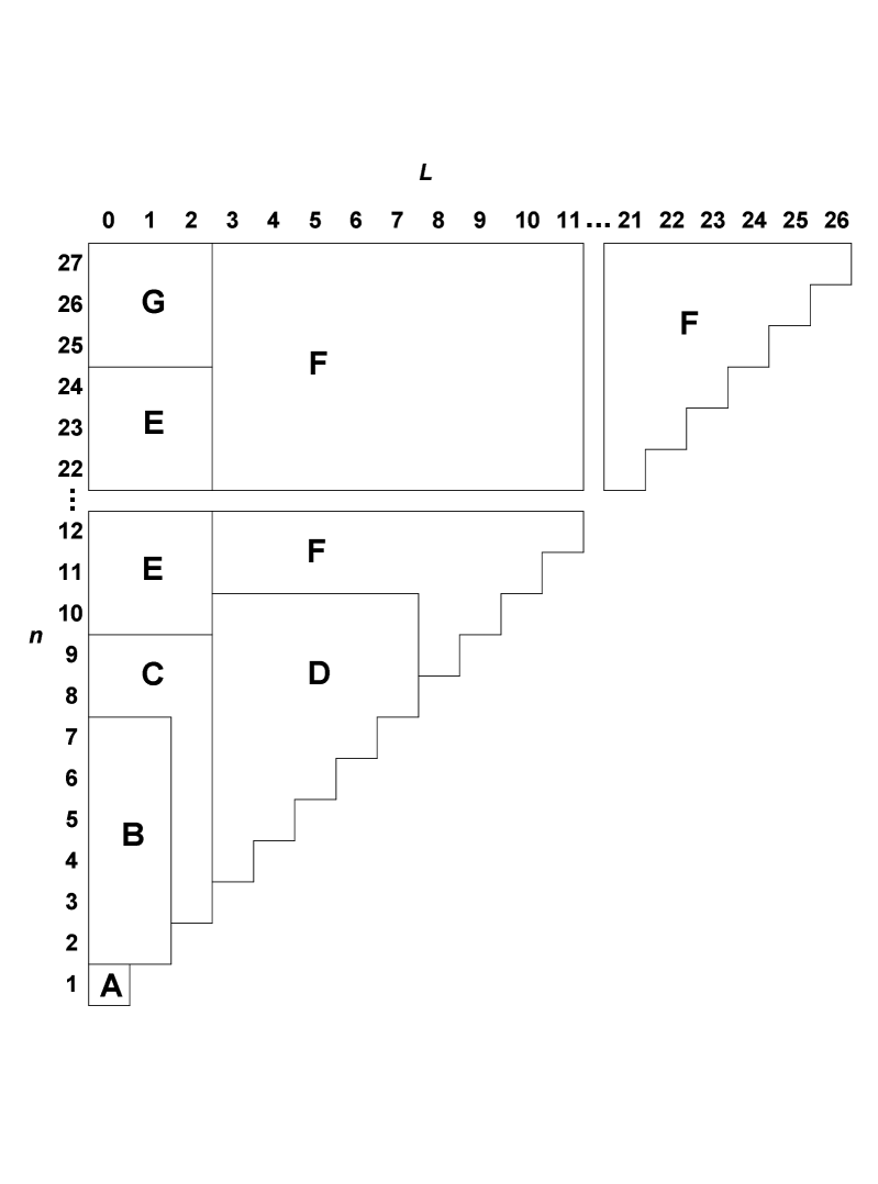
Figure 1: Graphical representation of the methods used for photoionization cross sections. The letters represent methods as follows: A) TOPbase; B) renormalized TOPbase (Section 2.3.7); C) renormalized Peach (Section 2.3.7); D) renormalized hydrogenic (Section 2.3.7); E) rescaled hydrogenic (Section 2.3.6); and F) pure hydrogenic (Section 2.2.4); G) rescaled hydrogenic (Section 2.3.1);

For the higher lying levels $n\leq 24,L\leq 2$, hydrogenic recombination rates (Burgess & Seaton 1960a, 1960b, hereafter BS60a and BS60b) are calculated and then scaled by the ratio of helium and hydrogen threshold photoionization cross sections. For levels with $n\geq 25$ and $L\leq 2$, hydrogenic recombination rates are used with scale factors given by HS98. For levels $n\leq 10$ and $L\geq 3$, or for all levels $L\geq 7$, pure hydrogenic recombination rates are used. Hydrogenic rates for $L\geq 4$ agree with those of helium to at least three figures (HS98). The methods used to calculate the radiative recombination rates for individual $nL$ levels are depicted in Figure 1.

2.3.2 Photoionization cross sections

The photoionization cross section for photons of arbitrary polarization in terms of the differential oscillator strength is given by (see, for example, Friedrich 1990)

$$\sigma(\varepsilon)=4\pi^{2}a_{0}^{2}\,\alpha_{\mathrm{fs}}\,\frac{df}{d\varepsilon}=(4.033643\times 10^{-18}\mathrm{~{}cm}^{2})\;\frac{df}{d\varepsilon}\;$$ (9)

where $a_{0}$ is the Bohr radius. For photoionization from an initial (lower) bound state with $n_{l},\ell_{l}$ to a final (upper) continuum state with angular momentum $\ell_{u}$, the non-$J$-resolved (mean) photoionization differential oscillator strength is

$$\frac{df_{n_{l}\ell_{l},\varepsilon\ell_{u}}}{d\varepsilon}=\frac{2\mu}{3\hbar}\omega\,\frac{\ell_{>}}{2\ell_{l}+1}\left({\int\limits_{0}^{\infty}{dr\;\phi^{\ast}_{n_{l}\ell_{l}}(r)\;r\;\Phi_{\varepsilon\ell_{u}}(r)}}\right)^{2}.$$ (10)

Here, the initial bound state radial wavefunction is $\phi_{n_{l}\ell_{l}}(r)$ and the final (energy normalized) continuum-state radial wavefunction is $\Phi_{\varepsilon\ell_{u}}(r)$.

2.3.3 TOPbase photoionization cross sections

For levels $n=2$ to $7$ and $L=0$ or $1$, the photoionization cross sections used for the calculation of the recombination rates are obtained from the Opacity Project (F87) as deposited in the database TOPbase (Cunto et al. 1993). These are labeled with B in Figure 1. The photoionization cross sections of F87 are ab initio close-coupling calculations using the $R$-matrix method (Berrington et al. 1974, 1978, 1987) of the scattering of an electron from a helium ion. For those photoionization cross sections missing from the database we use the method of P67.

2.3.4 Peach photoionization cross sections

For levels $n=3$ to $9$ and $L=0$ or $2$, the partial photoionization cross sections are obtained from P67. These levels are labeled with C in Figure 1. The method of P67 is based on the quantum defect representation of Coulomb wavefunctions and boundary conditions of BS60a. It is applicable for states with the initial bound-state principal quantum number $n_{i}\leq 12$ and may be used to calculate partial photoionization cross sections with initial orbital quantum number $\ell=L\leq 2$. These partial photoionization cross sections are sufficient to calculate the recombination coefficients for $S$, $P$, and $D$ states. A functional form $\nu(E)$ is first found from the quantum defects for each series to calculate the required first derivative of $\nu$ and the non-hydrogenic part of the continuum phase beyond the photoionization threshold.

The form of the partial photoionization cross section $\sigma_{\mathrm{p}}(\nu,\ell;\varepsilon,\ell\pm 1)$ is given by

$$\sigma_{\mathrm{p}}(\nu,\ell;\varepsilon,\ell\pm 1)=\frac{8{\kern 1.0pt}\alpha_{\mathrm{fs}}a_{0}^{2}\nu^{3}}{3\zeta(\nu,\ell)}(1+\nu^{2}\varepsilon)^{-3}\,C^{\ell}_{\ell\pm 1}\left[{G(\nu,\ell;\varepsilon,\ell\pm 1)\cos\,\pi(\nu+\mu^{\prime}(\varepsilon)+\chi(\nu,\ell;\varepsilon,\ell\pm 1))}\right]^{2}.$$ (11)

Here $\mu^{\prime}(\varepsilon)$ is the continuum-state quantum defect phase and $C^{\ell}_{\ell\pm 1}=\ell_{>}/(2\ell+1)$ are coefficients (BS60a) obtained from the integrations over spin and angular co-ordinates.  P67 tabulates the necessary amplitudes $G(\nu,\ell;\varepsilon,\ell\pm 1)$ and $\zeta(\nu,\ell)$ and the non-hydrogenic phase $\chi(\nu,\ell;\varepsilon,\ell\pm 1)$ for ejected-electron energies $\varepsilon\leq 2hcR_{\mathrm{He}^{+}}$. At the temperatures considered here, by far the largest contribution to the recombination rates is from the first few eV, so that ion-core excitations and two-electron processes do not contribute to the integral.

2.3.5 Hydrogenic photoionization cross sections

For levels in which $n$ and $L$ are large enough, the core electron fully screens the nucleus, and exact analytic hydrogenic cross sections are used to calculate recombination rates. These levels are labeled with D, E, F, and G in Figure 1. Cross sections for this process are given by BS60a, and the implementation described by Brocklehurst (1972) is used.

2.3.6 Hydrogenic cross sections

For $n>10$ and $L<4$, we use scaled hydrogenic cross sections. The scale factor is an extrapolation as $n\rightarrow\infty$ of the ratio $\alpha_{\mathrm{He}}(\gamma)/\alpha_{\mathrm{H}}(nL)$, where $\alpha_{\mathrm{He}}(\gamma)$ and $\alpha_{\mathrm{H}}(nL)$ are the helium and hydrogen recombination coefficients, respectively. We fit these series of ratios $\alpha_{\mathrm{He}}(\gamma)$/$\alpha_{\mathrm{H}}(nL)$ by

$$\frac{\alpha_{\mathrm{H}}}{\alpha_{\mathrm{He}}}=a+\frac{b}{n^{2}}+\frac{c}{n^{4}}$$ (12)

where the third term is only used for the ${}^{3}P$ series. Our results for $\alpha_{\mathrm{He}}$/$\alpha_{\mathrm{H}}$ agree well with HS98 at $n=25$ for the singlet and triplet $S$, $P$, and $F$ series but disagree for the singlet and triplet $D$ series by about 2.0%.

2.3.7 Renormalizing photoionization cross sections

HS98 concludes that neither the photoionization cross sections from Peach’s Coulomb method nor those of the Opacity Project are ideal. Extrapolation of the absorption oscillator strengths of D96, based on Seaton’s Theorem Seaton (1958) and as discussed in Section 2.2.2, to $E_{jl}=E_{l}$ yields the photoionization cross sections at threshold ($\varepsilon=0$). These differ, for $L\leq 3$, by up to $5.0\%$ from those of P67 and the Opacity Project. We use the extrapolated threshold values to renormalize the continuum cross sections. Similarly renormalized hydrogenic cross sections are used for levels $n\leq 10$ and $L\geq 3$.

2.3.8 $J$-resolved photoionization cross sections

The P67, TOPbase and hydrogenic photoionization cross sections are not $J$-resolved. The analysis used to find $J$-resolved in terms of non-$J$-resolved photoionization cross sections is similar to the above analysis of oscillator strengths. The (mean) partial photoionization cross section is given by

$$\sigma_{\mathrm{p}}(\gamma_{l},\gamma_{u};\omega)=\frac{2\mu\omega}{3\hbar}\sum\limits_{M_{u}=-J_{u}}^{J_{u}}\frac{1}{2J_{l}+1}\sum\limits_{M_{l}=-J_{l}}^{J_{l}}|\langle\,\phi_{\gamma_{l}M_{l}}|\vec{r}|\Phi_{{\gamma_{u}}{M_{u}}}\rangle|^{2}.$$ (13)

When the bound-free radial integrals can be explicitly calculated, the $J$-resolved (mean) total photoionization cross section may be written as

$$\sigma(\gamma;\omega)=\sum\limits_{{L_{u}}=L_{l}\pm 1}\frac{2\mu\omega}{3\hbar}\frac{L_{>}}{(2L_{l}+1)}\,\sum\limits_{J_{u}}(2{J_{u}}+1)\left\{\matrix{{L_{l}}&{1}&{L_{u}}\cr{J_{u}}&{S}&{J_{l}}\cr}\right\}^{2}\,\left({\int\limits_{0}^{\infty}{dr\;\phi_{\gamma_{l}}^{\ast}(r)\;r\;\Phi_{{\gamma_{u}}}(r)}}\right)^{2}.$$ (14)

Equation 14 cannot, however, be used to calculate $J$-resolved cross sections from pre-calculated non-$J$-resolved cross sections, such as those from TOPbase. In this case, we produce $J$-resolved cross sections by apportioning the non-$J$-resolved cross sections according to the statistical weight of the states within the lower term, as follows:

$$\sigma(\gamma;\omega)=\frac{2J+1}{(2L+1)(2S+1)}\sigma_{TOP}(nLS;\omega).$$ (15)

2.3.9 Recombination to levels with $n$ greater than $n_{\max}$

In the low density limit, an infinite number of levels $k$ must be considered. The largest principal quantum number $n$ for explicitly considered levels is $n_{\max}$. Simple truncation of the system at $n_{\max}$, however, would fail to account for the recombinations to and cascades from all higher levels, causing an underestimation of emission coefficients. The recombination remainder $\alpha_{\mathrm{rem}}$, the sum of the convergent infinite series of recombination to higher levels, must therefore be artificially added to the direct recombination of the explicitly treated levels. The recombination remainder is calculated by using an approximation method described by Seaton (1959).

While recombination coefficients into a given $n$ are largest for low to moderate angular momenta and then sharply decline for greater angular momenta, effective recombination into a given $n$—the sum of direct recombination and cascades from higher levels—will be distributed among $\ell$ very nearly according to statistical weight $2\ell+1$. In our treatment, we apportion $\alpha_{\mathrm{rem}}$ according to the statistical weights of the separate $\ell$ levels with $n=n_{\max}$ and add it to the direct recombination $\alpha(n_{\max},\ell)$ of the respective levels, so that the resultant recombination rate is given by

$$\alpha(n_{\max},\ell)\rightarrow\alpha(n_{\max},\ell)+\left({\frac{2\ell+1}{n_{\max}^{2}}}\right)\alpha_{\mathrm{rem}}.$$

.

The second term in the above sum, which we refer to here as “topoff”, is large compared with the direct recombination (first term), and the difference is greatest for high $\ell$ levels. (Levels having $\ell=n-1$ are called “yrast” levels; see Grover 1967.) In the low-density limit, an uncertainty is introduced by the addition of topoff, because the levels are not actually statistically distributed. This uncertainty is minimized by employing the largest possible $n_{\max}$.

3 Radiative Recombination Cascade Problem

3.1 Case A and Case B

Baker & Menzel (1938) proposed two limiting cases of Lyman line optical depth in the interstellar medium (ISM). The Case A approximation assumes that the line-emitting region is optically thin and that radiative excitation from the ground state is unimportant. The Case B approximation assumes that Lyman line photons originating from $n>2$ scatter often enough that they are degraded to Balmer lines and Ly$\alpha$. Baker & Menzel found that Case B more closely reproduced observations of hydrogen emission from the ISM than did Case A. In helium, singlet levels have the same Case A - Case B distinction, but triplet levels, having no resonance lines, do not. The present calculation considers only the Case B approximation.

3.2 Rate-equation formalism

In the steady-state, low-density, zero-incident-radiation limit we have the following balance equations for levels $k$ of $\mathrm{He}^{0}$:

$$n_{e}n_{\mathrm{He}^{+}}\alpha(k;T)=\sum\limits_{E_{l}<E_{k}}{n_{k}A_{kl}}-\sum\limits_{E_{j}>E_{k}}{n_{j}A_{jk}}$$ (16)

where $A_{pq}$ is the transition probability (s${}^{-1})$ from level $p$ to level $q$, $n_{e}$ and $n_{\mathrm{He}^{+}}$ are the local electron and singly ionized helium number densities (cm${}^{-3})$, $n_{k}$ is the number density of helium atoms in level $k$ (cm${}^{-3})$, and $\alpha(k;T)$ is the recombination coefficient (cm³ s${}^{-1})$ to level $k$ at temperature $T$(K).

The set of $k_{\max}$ balance equations (where $k_{\max}$ is the number of levels considered in the calculation) can be solved for the vector of level densities $(n_{1},n_{2},n_{3},\ldots,n_{k},\ldots,n_{k_{\max}})$. With the level densities known, local line emission coefficients $4\pi j_{\lambda}/n_{e}n_{\mathrm{He}^{+}}$ for the radiation at wavelength $\lambda=hc/E_{kl}$, where $E_{kl}=E_{k}-E_{l}$, are

$$\frac{4\pi j_{\lambda}}{n_{e}n_{\mathrm{He}^{+}}}=\frac{n_{k}}{n_{e}n_{\mathrm{He}^{+}}}A_{kl}E_{kl}$$ (17)

where $j_{\lambda}$ are the corresponding emissivities (erg cm^-3 s^-1). The emission coefficient is conventionally given in units of erg cm³ s^-1. (The conversion to SI units is 1 erg cm³ s${}^{-1}=10^{-13}$ J m³ s^-1.) The total intensity of the line (erg cm^-2 s^-1) is the local emissivity integrated over the depth of the line-emitting region.

4 Results and uncertainties

We discuss our results for a single prototype case with a temperature of $10,000$ K and with particle densities $n_{e}\,=1\mathrm{~{}cm}^{-3}$ and $n_{\mathrm{He}^{+}}\,=1\mathrm{~{}cm}^{-3}$. Collisional interactions are ignored in this low-density limit.

4.1 Absence of singlet-triplet mixing effects in multiplets

A comparison of the emission coefficients, $4\pi j_{\lambda}/n_{e}n_{\mathrm{He}^{+}}$, of the components of representative multiplets for singlet-triplet mixing and for pure $LS$-coupling is presented in Table 2: there are some differences. For transitions having $L_{l}=0$ or $1$, which encompasses all of the ultraviolet and most of the strongest visible and longer wavelength lines, the differences in the emission coefficients are negligibly small. Many of the emission coefficients of longer wavelength lines ($L_{l}\geq 2$) show a strong sensitivity to the presence of singlet-triplet mixing. Of course, intercombination lines ($\Delta S\neq 0$) are also then present. Large changes in emission coefficients when singlet-triplet mixing is included are almost entirely due to branching ratios as opposed to occupation numbers. Further, any small differences in the occupation numbers do not “accumulate” along cascade paths and affect subsequent emissions.

The Doppler widths at temperatures of order $10,000$ K, typical in the ISM, are such that, for most of the strongest IR and visible lines, the individual $J$ components are not resolvable. Thus, Table 2 also gives the summed multiplet emission coefficients. These are not significantly affected by including singlet-triplet mixing. Therefore, in the remaining sections we will use pure $LS$-coupling and provide multiplet emission coefficients.

4.2 Effects of topoff and $n_{\max}$ on convergence

The full problem with an infinite number of levels cannot be solved exactly. There are two aspects of the effect of truncation—the modeling of a finite number of levels—on our results: One is the choice of $n_{\max}$, the highest principal quantum number used. The other (topoff) is the way in which the recombination remainder $\alpha_{\mathrm{rem}}$ is distributed among $\ell$ values at $n_{\max}$. In particular, there is more than one reasonable approach to topoff, and these different approaches may lead to differences in the emission coefficients of certain lines.

These issues can be examined by comparing the results of the present calculation with those of a second independent non-$J$-resolved calculation, Cloudy (see Appendix A and Ferland et al. 1998). The approach to topoff used in Cloudy differs somewhat from that described in Section 2.3.9. The $J$-resolved calculation distributes $\alpha_{\mathrm{rem}}$ according to statistical weights, while Cloudy assumes the levels are populated according to statistical weight. These would be equivalent if the inverse lifetimes of these levels were proportional to statistical weight, which they are not.

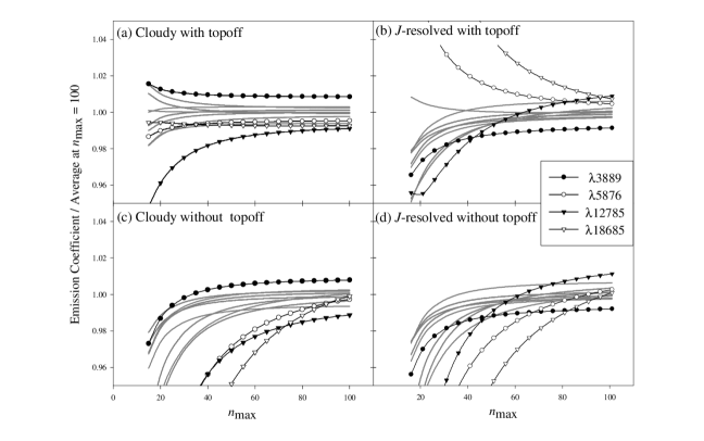
Figure 2: The effects of increasing $n_{\max}$ on the convergence of emission coefficients is shown. The emission coefficients are results from the two different model calculations with and without topoff as follows: a) Cloudy (Ferland et al. 1998) with topoff; b) $J$-resolved with topoff; c) Cloudy without topoff; and d) $J$-resolved without topoff. The average emission coefficient used to normalize the results is the average of the two model calculations at $n_{\max}=100$.

Both calculations are evaluated twice, with and without topoff. Figure 2 displays the emission coefficients of several strong optical and infrared lines, in each of the four cases, as a function of $n_{\max}$. Topoff is included in the top two panels but not in the bottom two. The left two panels show the results of Cloudy, and the right two show the results of the $J$-resolved calculations. We normalize each emission coefficient to the average emission coefficient at $n_{\max}=100$. In each panel, the four lines bearing symbols designate cases that exhibit the greatest disagreement or slowest convergence with increasing $n_{\max}$.

With topoff included, Cloudy converges more rapidly than the $J$-resolved code, a result of differing implementations of topoff. For most of the lines plotted, the difference between the two codes at $n_{\max}=100$ is less than $1\%$. With topoff not included, most lines again agree to better than $1\%$, although there are also significant outliers. The lines bearing symbols originate from yrast levels and their near neighbors. These levels are most affected by the inclusion of topoff and its method of implementation, due to the restrictive selection rules that govern their decays. An yrast level (with $l=n-1$) can only decay to one other yrast level (with $n^{\prime}=n-1$ and $l^{\prime}=n^{\prime}-1$) or to the level $n^{\prime}=n$, $l^{\prime}=n-2$ via a $\Delta n=0$ transition. The yrast-to-yrast decay is far more likely than the $\Delta n=0$ decay. Thus, an yrast-to-yrast decay most likely will be followed by another yrast-to-yrast decay. It follows that any fraction of the recombination remainder, $\alpha_{\mathrm{rem}}$, added to the yrast level at $n_{\max}$ increases the effective recombination of all lower yrast levels by nearly the same amount. Thus, the effects of including topoff are not yet negligible even at $n_{\max}=100$ for yrast levels. However, in a real atom at finite densities, collisions will dominate (Porter et al. 2005) the very highest $n$-levels and force the populations into LTE.

4.3 Effects of uncertainties in the atomic data

The lower two panels of Figure 2 show the two calculations without topoff out to $n_{\max}=100$. The majority of lines shown in the two lower panels of Figure 2 appear to have converged and show agreement to better than $1.0\%$. However, lines from yrast-to-yrast transitions (indicated by symbols in the figure) appear not to have converged for $n_{\max}=100$. For the lines which have converged, the differences are entirely due to the atomic data. There exist gaps in the atomic data that must be bridged, between the region where exact accurate variational results exist and the region where the hydrogenic approximation becomes applicable. The two codes use different reasonable approximations to bridge these gaps, and this introduces an uncertainty which we quantify here.

The Einstein $A$ coefficients introduce the lesser degree of uncertainty. Transitions between high-angular momentum levels are hydrogenic to a sufficient degree of accuracy. Transitions involving $S$, $P$, and $D$ levels involve different approximations, including semi-classical quantum defects and extrapolation from low-$n$ data.

Recombination coefficients, which are derived from photoionization cross sections, are the greater source of uncertainty. Cross sections for $10\leq n\leq 25$ and $L\leq 2$ are the least accurate of these.

4.4 Emission coefficients of representative He lines

Table 3 presents multiplet emission coefficients for lines satisfying the following criteria: $n_{u}\leq 15$, $\lambda<100\ \mu\mathrm{m}$, and $j_{\lambda}/j_{10830}\geq 10^{-3}$. Each emission coefficient is the average, with $n_{\max}=100$, of the results from Cloudy and the $J$-resolved code, with the individual fine-structure components in the $J$-resolved calculation summed. Column 4 gives these average emission coefficients without topoff, and Column 5 gives confidence estimates based on the differences between Cloudy and the $J$-resolved code, again without topoff. Columns 7 and 8 respectively present these values with topoff included. Confidence symbols correspond to percent difference between the results of Cloudy and the $J$-resolved code: AA, A, B, and C signify that the results differ by less than $0.1\%$, less than $1.0\%$, less than $5.0\%$, and more than $5.0\%$, respectively. Column 6 is the percent difference between columns 4 and 7.

In Table 4 we present our final values along with the lowest density $(n_{e}=100\mathrm{~{}cm}^{-3})$ case of BSS99. The small but unknown collisional contributions to the results of BSS99 prevent a rigorous comparison. Some transitions may also differ by a few percent because BSS99 did not scale the TOPbase photoionization cross sections to agree with accurate ab initio cross sections at threshold.

5 Conclusions

We reach the following conclusions:

A definitive test for the helium abundance produced in the Big Bang (Olive & Skillman 2004) requires that its abundance be measured to an accuracy of better than $1/2\%$. The requirement for the He I emission coefficients are similar. Several of the most important lines calculated here do not meet that accuracy requirement.

Improvements in the atomic data will be required to achieve that accuracy. Our final accuracy is limited by gaps in the atomic data, mainly photoionization cross sections for intermediate-$n$, low-$L$ levels. An extension of the bound-bound oscillator strengths for low-$L$ transitions will also improve further recombination-cascade calculations.

Singlet-triplet mixing does not affect intensities of multiplets, although intensities of lines within a multiplet can be strongly affected. There may be an effect at finite densities or with realistic radiative transfer.

Multiplets are not resolved in most astronomical sources since the intrinsic line widths are greater than the line splittings. It is not necessary to resolve fine structure in future calculations of the He I emission spectrum.

In the low-density limit there is an additional uncertainty introduced by the need to “top off” a finite numerical representation of the infinite-level atom. This uncertainty can amount to $1\%$ for yrast-to-yrast lines but will not occur in actual nebulae. These have densities high enough for collisional processes to force populations of very highly excited levels into statistical equilibrium.

The predictions in Table 3 (columns 7 & 8) can be used to identify those lines that are least affected by gaps in the atomic data. These lines should be used when precise helium abundances are the desired end product.

Both of the codes discussed here are freely available and open source. Cloudy can be downloaded from http://www.nublado.org, and the $J$-resolved code can be found at http://www.pa.uky.edu/$\sim$rporter.

We thank the NSF and NASA for support of this project through AST 03 07720 and NAG5-12020 and UK’s Center for Computational Sciences for a generous allocation of computer time. We also thank referee Peter Storey for his helpful suggestions.

Appendix A The non-$J$-resolved treatment in Cloudy

The recombination problem in the non-$J$-resolved code Cloudy (Ferland et al. 1998) was solved as follows:

Energies for levels not included in the calculations of D96 are calculated by assuming constant quantum defects for $n\geq 10$. For levels with $L\geq 8$, the quantum defects are calculated from a power law extrapolation of the lower $L$ defects at $n=10$. These differences are by far the most accurately known and the most consistent between Cloudy and the $J$-resolved code. In both calculations there is essentially no uncertainty due to energies.

Emission oscillator strengths for $n_{u}\geq 11$, not included in the calculations of D96, are calculated by the extrapolation method outlined in Section 2.2.2 for transitions with $n_{u}\geq 11$, $n_{l}\leq 5$, and both $L_{u}$ and $L_{l}\leq 2$. Emission oscillator strengths for hydrogenic transitions with $n_{u}\geq 11$, $n_{l}<n_{u}$, and both $L_{u}$ and $L_{l}\geq 2$, are calculated by the method of HB90 discussed in Section 2.2.4. All other oscillator strengths are calculated using the semi-classical quantum defect method of Drake (1996, Chapter 7). The probability for the forbidden transition $2{}^{1}P-2{}^{3}S$ is from Lach & Pachucki (2001). The most significant discrepancies (and uncertainties) in oscillator strengths between Cloudy and the $J$-resolved code are for levels with $n_{u}\geq 11$, $n_{l}>5$, and both $L_{l}$ and $L_{u}<2$.

We use fits to the TOPbase photoionization cross sections for the following levels: $n{}^{1,3}S$ for $n\leq 10$; $2{}^{3}P$ and $3{}^{3}P$; and $n^{1}$P for $n\leq 7$. P67 is used for the following levels: $n{}^{3}P$ for $4\leq n\leq 10$; and $n{}^{1,3}D$ for $n\leq 10$. All other cross sections are calculated using a scaled hydrogenic method as in Section 2.3.5. Cross sections for levels with $n\leq 4$ are rescaled to agree at threshold with the ab initio values calculated by HS98. For levels with $n=5$ they are rescaled to values computed by the extrapolation method outlined by HS98. Differences in photoionization cross sections between our two codes are most significant for levels with $L\leq 2$, while cross sections for levels with $L>2$ are essentially identical and have negligible uncertainties. Photoionization cross sections, and by extension recombination coefficients, are the greatest uncertainties in our calculations.

Cloudy treats topoff differently from the $J$-resolved code. Cloudy employs a “collapsed” level at $n_{\max}$ in which all of the individual $nLS$ terms are brought together as one pseudo-level. The recombination coefficient into this pseudo-level is the sum of recombination coefficients into the individual terms (calculated as in Section 2.3, with the changes in photoionization cross sections noted above) plus the recombination remainder. Transition probabilities from this pseudo-level are calculated as follows

$$A(n_{\max}\rightarrow n_{l},L_{l},S)=\frac{\sum\limits_{L_{u}=L_{l}\pm 1}{g_{L_{u},S}A(n_{\max},L_{u},S\rightarrow n_{l},L_{l},S)}}{\sum\limits_{L_{u}=L_{l}\pm 1}{g_{L_{u},S}}}$$ (A1)

This causes the collapsed level to behave exactly as if it were a set of resolved terms populated according to statistical weight.

Table 1: The method used to calculated the oscillator strengths depends on the upper and lower levels. KEY: A) D96 B) extrapolation of D96 C) R79 D) hydrogenic E) various including non-dipole transitions X) dipole transitions not included in Case B. The method used is independent of $S$ and $J$ except for transitions labeled with E as these will include non-dipole transitions.

n			2	3	4	5	6	7	8	9	10	11	12	13
	L		01	012	0123	01234	012345	0123456	01234567	012345678	0123456789	01234567891	012345678911	0123456789111
												0	01	012
lower
1	0		EE	.X.	.X..	.X...	.X....	.X.....	.X......	.X.......	.X........	.X.........	.X..........	.X...........
2	0		.E	.A.	.A..	.A...	.A....	.A.....	.A......	.A.......	.A........	.B.........	.B..........	.B...........
	1		..	A.A	A.A.	A.A..	A.A...	A.A....	A.A.....	A.A......	A.A.......	B.B........	B.B.........	B.B..........
3	0		..	.A.	.A..	.A...	.A....	.A.....	.A......	.A.......	.A........	.B.........	.B..........	.B...........
	1		..	...	A.A.	A.A..	A.A...	A.A....	A.A.....	A.A......	A.A.......	B.B........	B.B.........	B.B..........
	2		..	.A.	.A.A	.A.A.	.A.A..	.A.A...	.A.A....	.A.A.....	.A.A......	.B.B.......	.B.B........	.B.B.........
4	0		..	...	.A..	.A...	.A....	.A.....	.A......	.A.......	.A........	.B.........	.B..........	.B...........
	1		..	...	....	A.A..	A.A...	A.A....	A.A.....	A.A......	A.A.......	B.B........	B.B.........	B.B..........
	2		..	...	.A.A	.A.A.	.A.A..	.A.A...	.A.A....	.A.A.....	.A.A......	.B.B.......	.B.B........	.B.B.........
	3		..	...	....	..A.A	..A.A.	..A.A..	..A.A...	..A.A....	..A.A.....	..B.B......	..B.B.......	..B.B........
5	0		..	...	....	.A...	.A....	.A.....	.A......	.A.......	.A........	.C.........	.C..........	.C...........
	1		..	...	....	.....	A.A...	A.A....	A.A.....	A.A......	A.A.......	C.C........	C.C.........	C.C..........
	2		..	...	....	.A.A.	.A.A..	.A.A...	.A.A....	.A.A.....	.A.A......	.C.C.......	.C.C........	.C.C.........
	3		..	...	....	....A	..A.A.	..A.A..	..A.A...	..A.A....	..A.A.....	..C.C......	..C.C.......	..C.C........
	4		..	...	....	.....	...A.A	...A.A.	...A.A..	...A.A...	...A.A....	...D.D.....	...D.D......	...D.D.......
6	0		..	...	....	.....	.A....	.A.....	.A......	.A.......	.A........	.C.........	.C..........	.C...........
	1		..	...	....	.....	......	A.A....	A.A.....	A.A......	A.A.......	C.C........	C.C.........	C.C..........
	2		..	...	....	.....	.A.A..	.A.A...	.A.A....	.A.A.....	.A.A......	.C.C.......	.C.C........	.C.C.........
	3		..	...	....	.....	....A.	..A.A..	..A.A...	..A.A....	..A.A.....	..C.C......	..C.C.......	..C.C........
	4		..	...	....	.....	.....A	...A.A.	...A.A..	...A.A...	...A.A....	...C.C.....	...C.C......	...C.C.......
	5		..	...	....	.....	......	....A.A	....A.A.	....A.A..	....A.A...	....D.D....	....D.D.....	....D.D......
7	0		..	...	....	.....	......	.A.....	.A......	.A.......	.A........	.C.........	.C..........	.C...........
	1		..	...	....	.....	......	.......	A.A.....	A.A......	A.A.......	C.C........	C.C.........	C.C..........
	2		..	...	....	.....	......	.A.A...	.A.A....	.A.A.....	.A.A......	.C.C.......	.C.C........	.C.C.........
	3		..	...	....	.....	......	....A..	..A.A...	..A.A....	..A.A.....	..C.C......	..C.C.......	..C.C........
	4		..	...	....	.....	......	.....A.	...A.A..	...A.A...	...A.A....	...C.C.....	...C.C......	...C.C.......
	5		..	...	....	.....	......	......A	....A.A.	....A.A..	....A.A...	....C.C....	....C.C.....	....C.C......
	6		..	...	....	.....	......	.......	.....A.D	.....A.D.	.....A.D..	.....D.D...	.....D.D....	.....D.D.....
8	0		..	...	....	.....	......	.......	.A......	.A.......	.A........	.C.........	.C..........	.C...........
	1		..	...	....	.....	......	.......	........	A.A......	A.A.......	C.C........	C.C.........	C.C..........
	2		..	...	....	.....	......	.......	.A.A....	.A.A.....	.A.A......	.C.C.......	.C.C........	.C.C.........
	3		..	...	....	.....	......	.......	....A...	..A.A....	..A.A.....	..C.C......	..C.C.......	..C.C........
	4		..	...	....	.....	......	.......	.....A..	...A.A...	...A.A....	...C.C.....	...C.C......	...C.C.......
	5		..	...	....	.....	......	.......	......A.	....A.A..	....A.A...	....C.C....	....C.C.....	....C.C......
	6		..	...	....	.....	......	.......	.......C	.....A.D.	.....A.D..	.....C.D...	.....C.D....	.....C.D.....
	7		..	...	....	.....	......	.......	........	......A.D	......A.D.	......D.D..	......D.D...	......D.D....
9	0		..	...	....	.....	......	.......	........	.A.......	.A........	.C.........	.C..........	.C...........
	1		..	...	....	.....	......	.......	........	.........	A.A.......	C.C........	C.C.........	C.C..........
	2		..	...	....	.....	......	.......	........	.A.A.....	.A.A......	.C.C.......	.C.C........	.C.C.........
	3		..	...	....	.....	......	.......	........	....A....	..A.A.....	..C.C......	..C.C.......	..C.C........
	4		..	...	....	.....	......	.......	........	.....A...	...A.A....	...C.C.....	...C.C......	...C.C.......
	5		..	...	....	.....	......	.......	........	......A..	....A.A...	....C.C....	....C.C.....	....C.C......
	6		..	...	....	.....	......	.......	........	.......C.	.....A.D..	.....C.D...	.....C.D....	.....C.D.....
	7		..	...	....	.....	......	.......	........	........C	......A.D.	......D.D..	......D.D...	......D.D....
9	8		..	...	....	.....	......	.......	........	.........	.......D.D	.......D.D.	.......D.D..	.......D.D...
10	0		..	...	....	.....	......	.......	........	.........	.A........	.C.........	.C..........	.C...........
	1		..	...	....	.....	......	.......	........	.........	..........	C.C........	C.C.........	C.C..........
	2		..	...	....	.....	......	.......	........	.........	.A.A......	.C.C.......	.C.C........	.C.C.........
	3		..	...	....	.....	......	.......	........	.........	....A.....	..C.C......	..C.C.......	..C.C........
	4		..	...	....	.....	......	.......	........	.........	.....A....	...C.C.....	...C.C......	...C.C.......
	5		..	...	....	.....	......	.......	........	.........	......A...	....C.C....	....C.C.....	....C.C......
	6		..	...	....	.....	......	.......	........	.........	.......C..	.....C.D...	.....C.D....	.....C.D.....
	7		..	...	....	.....	......	.......	........	.........	........C.	......D.D..	......D.D...	......D.D....
	8		..	...	....	.....	......	.......	........	.........	.........C	.......D.D.	.......D.D..	.......D.D...
	9		..	...	....	.....	......	.......	........	.........	..........	........D.D	........D.D.	........D.D..
11	0		..	...	....	.....	......	.......	........	.........	..........	.C.........	.C..........	.C...........
	1		..	...	....	.....	......	.......	........	.........	..........	...........	C.C.........	C.C..........
	2		..	...	....	.....	......	.......	........	.........	..........	.C.C.......	.C.C........	.C.C.........
	3		..	...	....	.....	......	.......	........	.........	..........	....C......	..C.C.......	..C.C........
	4		..	...	....	.....	......	.......	........	.........	..........	.....C.....	...C.C......	...C.C.......
	5		..	...	....	.....	......	.......	........	.........	..........	......C....	....C.C.....	....C.C......
	6		..	...	....	.....	......	.......	........	.........	..........	.......C...	.....C.D....	.....C.D.....
	7		..	...	....	.....	......	.......	........	.........	..........	........C..	......D.D...	......D.D....
	8		..	...	....	.....	......	.......	........	.........	..........	.........C.	.......D.D..	.......D.D...
	9		..	...	....	.....	......	.......	........	.........	..........	..........C	........D.D.	........D.D..
	10		..	...	....	.....	......	.......	........	.........	..........	...........	.........D.D	.........D.D.
12	0		..	...	....	.....	......	.......	........	.........	..........	...........	.C..........	.C...........
	1		..	...	....	.....	......	.......	........	.........	..........	...........	............	C.C..........
	2		..	...	....	.....	......	.......	........	.........	..........	...........	.C.C........	.C.C.........
	3		..	...	....	.....	......	.......	........	.........	..........	...........	....C.......	..C.C........
	4		..	...	....	.....	......	.......	........	.........	..........	...........	.....C......	...C.C.......
	5		..	...	....	.....	......	.......	........	.........	..........	...........	......C.....	....C.C......
	6		..	...	....	.....	......	.......	........	.........	..........	...........	.......C....	.....C.D.....
	7		..	...	....	.....	......	.......	........	.........	..........	...........	........C...	......D.D....
	8		..	...	....	.....	......	.......	........	.........	..........	...........	.........C..	.......D.D...
	9		..	...	....	.....	......	.......	........	.........	..........	...........	..........C.	........D.D..
	10		..	...	....	.....	......	.......	........	.........	..........	...........	...........C	.........D.D.
	11		..	...	....	.....	......	.......	........	.........	..........	...........	............	..........D.D

Table 2: Comparison of emission coefficients, $4\pi j_{\lambda}/n_{e}n_{\mathrm{He}^{+}}$ for representative multiplets $3\,{}^{1,3}D$ – $2\,{}^{1,3}P$ and $4\,{}^{1,3}F$ – $3\,{}^{1,3}D$ assuming pure $LS$-coupling and $ST$-mixing. The calculated emission coefficients of the component lines that comprise the above multiplets are given. The component line emission coefficients are summed to show the observable multiplet emission coefficients. Although small differences can be seen in the individual components, the multiplet sums are insensitive to $ST$-mixing. These calculations where carried out with $n_{\max}=100$.

Wavelength (Air)	Transition	$LS$-coupling emiss. coeff.	$ST$-mixing emiss. coeff.	Ratio of emiss. coeff.
Å		$\mathrm{erg~{}cm}^{3}\mathrm{~{}s}^{-1}$	$\mathrm{erg~{}cm}^{3}\mathrm{~{}s}^{-1}$	$LS$-coupling/$ST$-mixing
5874.456	$3\,{}^{1}D_{2}$ – $2\,{}^{3}P_{2}$	—	3.625369E-30	—
5874.483	$3\,{}^{1}D_{2}$ – $2\,{}^{3}P_{1}$	—	1.036918E-29	—
5875.621	$3\,{}^{3}D_{1}$ – $2\,{}^{3}P_{2}$	9.215998E-28	9.216010E-28	1.0000
5875.636	$3\,{}^{3}D_{2}$ – $2\,{}^{3}P_{2}$	1.382263E-26	1.382984E-26	0.9995
5875.637	$3\,{}^{3}D_{3}$ – $2\,{}^{3}P_{2}$	7.740541E-26	7.741031E-26	0.9999
5875.648	$3\,{}^{3}D_{1}$ – $2\,{}^{3}P_{1}$	1.382384E-26	1.382385E-26	1.0000
5875.663	$3\,{}^{3}D_{2}$ – $2\,{}^{3}P_{1}$	4.146730E-26	4.148941E-26	0.9995
5875.989	$3\,{}^{3}D_{1}$ – $2\,{}^{3}P_{0}$	1.842857E-26	1.842860E-26	1.0000
Sum	$3\,{}^{3}D$ – $2\,{}^{3}P$	1.658693E-25	1.659176E-25	0.9997
6678.180	$3\,{}^{1}D_{2}$ – $2\,{}^{1}P_{1}$	4.713582E-26	4.713351E-26	1.0000
6679.686	$3\,{}^{3}D_{1}$ – $2\,{}^{1}P_{1}$	—	7.287124E-34	—
6679.705	$3\,{}^{3}D_{2}$ – $2\,{}^{1}P_{1}$	—	1.039168E-29	—
Sum	$3\,{}^{1}D$ – $2\,{}^{1}P$	4.713582E-26	4.714390E-26	0.9998
18685.14	$4\,{}^{1}F_{3}$ – $3\,{}^{3}D_{3}$	—	3.080526E-28	—
18685.15	$4\,{}^{1}F_{3}$ – $3\,{}^{3}D_{2}$	—	2.357295E-27	—
18685.17	$4\,{}^{3}F_{2}$ – $3\,{}^{3}D_{3}$	2.410942E-29	2.410945E-29	1.0000
18685.18	$4\,{}^{3}F_{2}$ – $3\,{}^{3}D_{2}$	8.438345E-28	8.436298E-28	1.0002
18685.20	$4\,{}^{3}F_{4}$ – $3\,{}^{3}D_{3}$	9.762777E-27	9.762664E-27	1.0000
18685.23	$4\,{}^{3}F_{3}$ – $3\,{}^{3}D_{3}$	8.437227E-28	5.359178E-28	1.5744
18685.23	$4\,{}^{3}F_{3}$ – $3\,{}^{3}D_{2}$	6.749771E-27	4.394646E-27	1.5359
18685.33	$4\,{}^{3}F_{2}$ – $3\,{}^{3}D_{1}$	4.556594E-27	4.556599E-27	1.0000
Sum	$4\,{}^{3}F$ – $3\,{}^{3}D$	2.278081E-26	2.278291E-26	0.9999
18697.10	$4\,{}^{1}F_{3}$ – $3\,{}^{1}D_{2}$	7.589393E-27	4.925742E-27	1.5408
18697.12	$4\,{}^{3}F_{2}$ – $3\,{}^{1}D_{2}$	—	2.052122E-31	—
18697.18	$4\,{}^{3}F_{3}$ – $3\,{}^{1}D_{2}$	—	2.661372E-27	—
Sum	$4\,{}^{1}F$ – $3\,{}^{1}D$	7.589393E-27	7.587319E-27	1.0003

Table 3: Average emission coefficients, $4\pi j_{\lambda}/n_{e}n_{\mathrm{He}^{+}}$ in lines meeting the simultaneous criteria: $n_{u}\leq 15$, $\lambda<100\ \mu$m, and $j_{\lambda}/j_{10830}\geq 10^{-3}$. The confidence codes indicate the percent difference between the results of the two models: AA, A, B, and C correspond to a difference of less than 0.1%, less than 1.0%, less than 5.0%, and more than 5.0%, respectively.

			Emiss. coeff.			Emiss. coeff.
Wavelength (Air)	$n\,{}^{2S+1}\!L$	$n\,{}^{2S+1}\!L$	“no topoff”	Confidence	% diff.	“topoff”	Confidence
Å	upper	lower	$\mathrm{erg~{}cm}^{3}\mathrm{~{}s}^{-1}$			$\mathrm{erg~{}cm}^{3}\mathrm{~{}s}^{-1}$
2633	$15\;{}^{3}P$	$2\;{}^{3}S$	8.907E-28	B	0.05%	8.911E-28	B
2638	$14\;{}^{3}P$	$2\;{}^{3}S$	1.095E-27	B	0.05%	1.096E-27	B
2645	$13\;{}^{3}P$	$2\;{}^{3}S$	1.368E-27	B	0.05%	1.369E-27	B
2653	$12\;{}^{3}P$	$2\;{}^{3}S$	1.740E-27	B	0.05%	1.741E-27	B
2663	$11\;{}^{3}P$	$2\;{}^{3}S$	2.263E-27	B	0.05%	2.264E-27	B
2677	$10\;{}^{3}P$	$2\;{}^{3}S$	3.027E-27	B	0.04%	3.029E-27	B
2696	$9\;{}^{3}P$	$2\;{}^{3}S$	4.168E-27	A	0.04%	4.170E-27	AA
2723	$8\;{}^{3}P$	$2\;{}^{3}S$	6.036E-27	A	0.04%	6.039E-27	AA
2764	$7\;{}^{3}P$	$2\;{}^{3}S$	9.127E-27	A	0.04%	9.131E-27	AA
2829	$6\;{}^{3}P$	$2\;{}^{3}S$	1.487E-26	A	0.04%	1.488E-26	A
2945	$5\;{}^{3}P$	$2\;{}^{3}S$	2.655E-26	A	0.05%	2.657E-26	A
3176	$14\;{}^{1}P$	$2\;{}^{1}S$	2.944E-28	C	0.06%	2.946E-28	B
3185	$13\;{}^{1}P$	$2\;{}^{1}S$	3.689E-28	B	0.06%	3.691E-28	B
3188	$4\;{}^{3}P$	$2\;{}^{3}S$	5.561E-26	A	0.06%	5.564E-26	A
3197	$12\;{}^{1}P$	$2\;{}^{1}S$	4.703E-28	B	0.06%	4.706E-28	B
3212	$11\;{}^{1}P$	$2\;{}^{1}S$	6.121E-28	B	0.05%	6.125E-28	B
3231	$10\;{}^{1}P$	$2\;{}^{1}S$	8.170E-28	B	0.05%	8.174E-28	B
3258	$9\;{}^{1}P$	$2\;{}^{1}S$	1.119E-27	A	0.05%	1.119E-27	A
3297	$8\;{}^{1}P$	$2\;{}^{1}S$	1.607E-27	A	0.05%	1.608E-27	A
3355	$7\;{}^{1}P$	$2\;{}^{1}S$	2.409E-27	A	0.05%	2.410E-27	A
3448	$6\;{}^{1}P$	$2\;{}^{1}S$	3.869E-27	B	0.04%	3.870E-27	A
3479	$15\;{}^{3}D$	$2\;{}^{3}P$	9.696E-28	B	0.09%	9.704E-28	B
3488	$14\;{}^{3}D$	$2\;{}^{3}P$	1.193E-27	B	0.09%	1.194E-27	B
3499	$13\;{}^{3}D$	$2\;{}^{3}P$	1.490E-27	B	0.09%	1.491E-27	B
3513	$12\;{}^{3}D$	$2\;{}^{3}P$	1.896E-27	B	0.08%	1.897E-27	B
3531	$11\;{}^{3}D$	$2\;{}^{3}P$	2.465E-27	B	0.08%	2.467E-27	B
3554	$10\;{}^{3}D$	$2\;{}^{3}P$	3.324E-27	B	0.08%	3.327E-27	B
3587	$9\;{}^{3}D$	$2\;{}^{3}P$	4.575E-27	A	0.08%	4.579E-27	A
3599	$9\;{}^{3}S$	$2\;{}^{3}P$	3.057E-28	C	0.02%	3.058E-28	C
3614	$5\;{}^{1}P$	$2\;{}^{1}S$	6.859E-27	A	0.06%	6.864E-27	A
3634	$8\;{}^{3}D$	$2\;{}^{3}P$	6.574E-27	A	0.08%	6.579E-27	A
3652	$8\;{}^{3}S$	$2\;{}^{3}P$	4.538E-28	C	0.02%	4.539E-28	C
3705	$7\;{}^{3}D$	$2\;{}^{3}P$	9.934E-27	A	0.08%	9.942E-27	A
3733	$7\;{}^{3}S$	$2\;{}^{3}P$	7.290E-28	B	0.03%	7.292E-28	B
3756	$14\;{}^{1}D$	$2\;{}^{1}P$	3.141E-28	A	0.09%	3.144E-28	A
3769	$13\;{}^{1}D$	$2\;{}^{1}P$	3.924E-28	A	0.09%	3.928E-28	A
3785	$12\;{}^{1}D$	$2\;{}^{1}P$	4.993E-28	A	0.09%	4.997E-28	A
3806	$11\;{}^{1}D$	$2\;{}^{1}P$	6.491E-28	A	0.09%	6.497E-28	A
3820	$6\;{}^{3}D$	$2\;{}^{3}P$	1.613E-26	A	0.09%	1.614E-26	A
3834	$10\;{}^{1}D$	$2\;{}^{1}P$	8.577E-28	B	0.09%	8.584E-28	B
3868	$6\;{}^{3}S$	$2\;{}^{3}P$	1.263E-27	B	0.03%	1.263E-27	B
3872	$9\;{}^{1}D$	$2\;{}^{1}P$	1.182E-27	A	0.09%	1.183E-27	A
3889	$3\;{}^{3}P$	$2\;{}^{3}S$	1.380E-25	B	0.07%	1.381E-25	B
3927	$8\;{}^{1}D$	$2\;{}^{1}P$	1.704E-27	A	0.09%	1.705E-27	A
3965	$4\;{}^{1}P$	$2\;{}^{1}S$	1.397E-26	A	0.06%	1.398E-26	A
4009	$7\;{}^{1}D$	$2\;{}^{1}P$	2.585E-27	A	0.09%	2.587E-27	A
4024	$7\;{}^{1}S$	$2\;{}^{1}P$	3.065E-28	A	0.05%	3.067E-28	A
4026	$5\;{}^{3}D$	$2\;{}^{3}P$	2.898E-26	A	0.10%	2.901E-26	AA
4121	$5\;{}^{3}S$	$2\;{}^{3}P$	2.490E-27	B	0.04%	2.491E-27	B
4144	$6\;{}^{1}D$	$2\;{}^{1}P$	4.225E-27	A	0.09%	4.229E-27	A
4169	$6\;{}^{1}S$	$2\;{}^{1}P$	5.212E-28	A	0.05%	5.215E-28	A
4388	$5\;{}^{1}D$	$2\;{}^{1}P$	7.669E-27	A	0.10%	7.677E-27	A
4438	$5\;{}^{1}S$	$2\;{}^{1}P$	1.003E-27	A	0.04%	1.004E-27	A
4472	$4\;{}^{3}D$	$2\;{}^{3}P$	6.102E-26	A	0.13%	6.110E-26	A
4713	$4\;{}^{3}S$	$2\;{}^{3}P$	6.426E-27	A	0.04%	6.429E-27	A
4922	$4\;{}^{1}D$	$2\;{}^{1}P$	1.649E-26	A	0.14%	1.651E-26	A
5016	$3\;{}^{1}P$	$2\;{}^{1}S$	3.506E-26	A	0.08%	3.508E-26	A
5048	$4\;{}^{1}S$	$2\;{}^{1}P$	2.416E-27	A	0.04%	2.417E-27	A
5876	$3\;{}^{3}D$	$2\;{}^{3}P$	1.627E-25	A	1.47%	1.651E-25	A
6678	$3\;{}^{1}D$	$2\;{}^{1}P$	4.620E-26	A	1.51%	4.691E-26	A
7065	$3\;{}^{3}S$	$2\;{}^{3}P$	2.866E-26	A	0.05%	2.867E-26	A
7281	$3\;{}^{1}S$	$2\;{}^{1}P$	8.712E-27	A	0.05%	8.716E-27	A
7298	$9\;{}^{3}P$	$3\;{}^{3}S$	3.301E-28	A	0.04%	3.303E-28	AA
7500	$8\;{}^{3}P$	$3\;{}^{3}S$	4.627E-28	A	0.04%	4.629E-28	AA
7816	$7\;{}^{3}P$	$3\;{}^{3}S$	6.644E-28	A	0.04%	6.647E-28	AA
8362	$6\;{}^{3}P$	$3\;{}^{3}S$	9.894E-28	A	0.04%	9.898E-28	A
8444	$11\;{}^{3}D$	$3\;{}^{3}P$	3.307E-28	B	0.08%	3.309E-28	B
8582	$14\;{}^{3}F$	$3\;{}^{3}D$	3.169E-28	A	0.14%	3.174E-28	A
8583	$10\;{}^{3}D$	$3\;{}^{3}P$	4.407E-28	B	0.08%	4.410E-28	B
8648	$13\;{}^{3}F$	$3\;{}^{3}D$	3.977E-28	A	0.13%	3.982E-28	A
8733	$12\;{}^{3}F$	$3\;{}^{3}D$	5.089E-28	A	0.13%	5.096E-28	A
8777	$9\;{}^{3}D$	$3\;{}^{3}P$	5.965E-28	A	0.08%	5.970E-28	A
8845	$11\;{}^{3}F$	$3\;{}^{3}D$	6.665E-28	A	0.14%	6.674E-28	A
8997	$10\;{}^{3}F$	$3\;{}^{3}D$	8.999E-28	AA	0.14%	9.012E-28	A
9000	$10\;{}^{1}F$	$3\;{}^{1}D$	3.000E-28	AA	0.14%	3.004E-28	A
9063	$8\;{}^{3}D$	$3\;{}^{3}P$	8.365E-28	A	0.08%	8.372E-28	A
9210	$9\;{}^{3}F$	$3\;{}^{3}D$	1.260E-27	A	0.14%	1.262E-27	A
9213	$9\;{}^{1}F$	$3\;{}^{1}D$	4.200E-28	A	0.14%	4.206E-28	A
9464	$5\;{}^{3}P$	$3\;{}^{3}S$	1.468E-27	A	0.05%	1.469E-27	A
9517	$7\;{}^{3}D$	$3\;{}^{3}P$	1.217E-27	A	0.08%	1.218E-27	A
9526	$8\;{}^{3}F$	$3\;{}^{3}D$	1.843E-27	A	0.15%	1.846E-27	A
9529	$8\;{}^{1}F$	$3\;{}^{1}D$	6.142E-28	A	0.15%	6.151E-28	A
9603	$6\;{}^{1}P$	$3\;{}^{1}S$	3.567E-28	B	0.04%	3.569E-28	A
10028	$7\;{}^{3}F$	$3\;{}^{3}D$	2.864E-27	A	0.16%	2.869E-27	A
10031	$7\;{}^{1}F$	$3\;{}^{1}D$	9.546E-28	A	0.16%	9.561E-28	A
10138	$7\;{}^{1}D$	$3\;{}^{1}P$	3.883E-28	A	0.09%	3.887E-28	A
10311	$6\;{}^{3}D$	$3\;{}^{3}P$	1.852E-27	A	0.09%	1.854E-27	A
10830	$2\;{}^{3}P$	$2\;{}^{3}S$	2.705E-25	AA	0.53%	2.720E-25	AA
10913	$6\;{}^{3}F$	$3\;{}^{3}D$	4.853E-27	A	0.18%	4.862E-27	AA
10917	$6\;{}^{1}F$	$3\;{}^{1}D$	1.617E-27	A	0.18%	1.620E-27	AA
10997	$6\;{}^{3}P$	$3\;{}^{3}D$	2.812E-28	A	0.04%	2.813E-28	A
11013	$5\;{}^{1}P$	$3\;{}^{1}S$	5.475E-28	A	0.06%	5.479E-28	A
11045	$6\;{}^{1}D$	$3\;{}^{1}P$	5.993E-28	A	0.09%	5.999E-28	A
11969	$5\;{}^{3}D$	$3\;{}^{3}P$	2.923E-27	A	0.10%	2.926E-27	AA
12527	$4\;{}^{3}P$	$3\;{}^{3}S$	1.781E-27	A	0.06%	1.782E-27	A
12785	$5\;{}^{3}F$	$3\;{}^{3}D$	9.454E-27	B	0.27%	9.480E-27	B
12790	$5\;{}^{1}F$	$3\;{}^{1}D$	3.150E-27	B	0.27%	3.158E-27	B
12846	$5\;{}^{3}S$	$3\;{}^{3}P$	4.900E-28	B	0.04%	4.902E-28	B
12968	$5\;{}^{1}D$	$3\;{}^{1}P$	9.704E-28	A	0.10%	9.714E-28	A
12985	$5\;{}^{3}P$	$3\;{}^{3}D$	5.135E-28	A	0.05%	5.138E-28	A
15084	$4\;{}^{1}P$	$3\;{}^{1}S$	7.424E-28	A	0.06%	7.429E-28	A
17002	$4\;{}^{3}D$	$3\;{}^{3}P$	4.315E-27	A	0.13%	4.321E-27	A
17330	$10\;{}^{3}F$	$4\;{}^{3}D$	2.863E-28	AA	0.14%	2.867E-28	A
17352	$10\;{}^{3}G$	$4\;{}^{3}F$	3.424E-28	AA	0.23%	3.432E-28	A
18139	$9\;{}^{3}F$	$4\;{}^{3}D$	3.914E-28	A	0.14%	3.919E-28	A
18163	$9\;{}^{3}G$	$4\;{}^{3}F$	4.922E-28	A	0.24%	4.934E-28	A
18685	$4\;{}^{3}F$	$3\;{}^{3}D$	2.190E-26	A	3.18%	2.261E-26	B
18697	$4\;{}^{1}F$	$3\;{}^{1}D$	7.296E-27	A	3.18%	7.535E-27	B
19089	$4\;{}^{1}D$	$3\;{}^{1}P$	1.523E-27	A	0.14%	1.525E-27	A
19406	$8\;{}^{3}F$	$4\;{}^{3}D$	5.515E-28	A	0.15%	5.523E-28	A
19434	$8\;{}^{3}G$	$4\;{}^{3}F$	7.446E-28	A	0.27%	7.466E-28	AA
19543	$4\;{}^{3}P$	$3\;{}^{3}D$	1.038E-27	A	0.06%	1.039E-27	A
21118	$4\;{}^{3}S$	$3\;{}^{3}P$	9.811E-28	A	0.04%	9.815E-28	A
21130	$4\;{}^{1}S$	$3\;{}^{1}P$	3.915E-28	A	0.04%	3.917E-28	A
21608	$7\;{}^{3}F$	$4\;{}^{3}D$	8.054E-28	A	0.16%	8.067E-28	A
21641	$7\;{}^{3}G$	$4\;{}^{3}F$	1.216E-27	A	0.33%	1.220E-27	A
21642	$7\;{}^{1}G$	$4\;{}^{1}F$	4.053E-28	A	0.33%	4.066E-28	A
24727	$6\;{}^{3}D$	$4\;{}^{3}P$	3.140E-28	A	0.09%	3.143E-28	A
26185	$6\;{}^{3}F$	$4\;{}^{3}D$	1.207E-27	A	0.18%	1.210E-27	AA
26198	$6\;{}^{1}F$	$4\;{}^{1}D$	4.028E-28	A	0.18%	4.035E-28	AA
26234	$6\;{}^{3}G$	$4\;{}^{3}F$	2.253E-27	B	0.54%	2.265E-27	B
26234	$6\;{}^{1}G$	$4\;{}^{1}F$	7.508E-28	B	0.54%	7.549E-28	B
37026	$5\;{}^{3}D$	$4\;{}^{3}P$	3.475E-28	A	0.10%	3.479E-28	AA
37372	$8\;{}^{3}G$	$5\;{}^{3}F$	3.330E-28	A	0.27%	3.339E-28	AA
37378	$8\;{}^{3}H$	$5\;{}^{3}G$	3.527E-28	A	0.59%	3.548E-28	A
40366	$5\;{}^{3}F$	$4\;{}^{3}D$	1.693E-27	B	0.27%	1.697E-27	B
40398	$5\;{}^{1}F$	$4\;{}^{1}D$	5.646E-28	B	0.27%	5.662E-28	B
40479	$5\;{}^{3}G$	$4\;{}^{3}F$	4.660E-27	A	6.36%	4.976E-27	B
40479	$5\;{}^{1}G$	$4\;{}^{1}F$	1.553E-27	A	6.36%	1.658E-27	B
42946	$3\;{}^{3}P$	$3\;{}^{3}S$	1.416E-27	B	0.07%	1.417E-27	B
46493	$7\;{}^{3}G$	$5\;{}^{3}F$	4.801E-28	A	0.33%	4.817E-28	A
46503	$7\;{}^{3}H$	$5\;{}^{3}G$	6.495E-28	C	1.03%	6.562E-28	B
74517	$6\;{}^{3}G$	$5\;{}^{3}F$	6.383E-28	B	0.54%	6.418E-28	B
74541	$6\;{}^{3}H$	$5\;{}^{3}G$	1.238E-27	B	11.73%	1.403E-27	B
74541	$6\;{}^{1}H$	$5\;{}^{1}G$	4.126E-28	B	11.74%	4.675E-28	B
123631	$7\;{}^{3}I$	$6\;{}^{3}H$	3.763E-28	C	20.21%	4.716E-28	B

Table 4: Comparison of the present results with those of the lowest density ($100$ cm^-3) case of BSS99. The BSS99 results include collision contributions not considered in this work (see text).

Wavelength (Air)	$n\,{}^{2S+1}\!L$	$n\,{}^{2S+1}\!L$	Present	BSS99	% diff.
Å	upper	lower	$\mathrm{erg~{}cm}^{3}\mathrm{~{}s}^{-1}$	$\mathrm{erg~{}cm}^{3}\mathrm{~{}s}^{-1}$
$\lambda$			$4\pi j_{\lambda}/n_{e}n_{\mathrm{He}^{+}}$	$4\pi j_{\lambda}/n_{e}n_{\mathrm{He}^{+}}$
2945	$5\,{}^{3}P$	$2\,{}^{3}S$	2.657E-26	2.70E-26	1.6%
3188	$4\,{}^{3}P$	$2\,{}^{3}S$	5.564E-26	5.62E-26	1.0%
3614	$5\,{}^{1}P$	$2\,{}^{1}S$	6.864E-27	6.78E-27	-1.2%
3889	$3\,{}^{3}P$	$2\,{}^{3}S$	1.381E-25	1.37E-25	-0.8%
3965	$4\,{}^{1}P$	$2\,{}^{1}S$	1.398E-26	1.39E-26	-0.5%
4026	$5\,{}^{3}D$	$2\,{}^{3}P$	2.901E-26	2.86E-26	-1.4%
4121	$5\,{}^{3}S$	$2\,{}^{3}P$	2.491E-27	2.46E-27	-1.3%
4388	$5\,{}^{1}D$	$2\,{}^{1}P$	7.677E-27	7.58E-27	-1.3%
4438	$5\,{}^{1}S$	$2\,{}^{1}P$	1.004E-27	1.05E-27	4.4%
4472	$4\,{}^{3}D$	$2\,{}^{3}P$	6.110E-26	6.16E-26	0.8%
4713	$4\,{}^{3}S$	$2\,{}^{3}P$	6.429E-27	6.47E-27	0.6%
4922	$4\,{}^{1}D$	$2\,{}^{1}P$	1.651E-26	1.64E-26	-0.7%
5016	$3\,{}^{1}P$	$2\,{}^{1}S$	3.508E-26	3.49E-26	-0.5%
5048	$4\,{}^{1}S$	$2\,{}^{1}P$	2.417E-27	2.53E-27	4.5%
5876	$3\,{}^{3}D$	$2\,{}^{3}P$	1.651E-25	1.69E-25	2.3%
6678	$3\,{}^{1}D$	$2\,{}^{1}P$	4.691E-26	4.79E-26	2.1%
7065	$3\,{}^{3}S$	$2\,{}^{3}P$	2.867E-26	2.96E-26	3.1%
7281	$3\,{}^{1}S$	$2\,{}^{1}P$	8.716E-27	8.99E-27	3.0%
9464	$5\,{}^{3}P$	$3\,{}^{3}S$	1.469E-27	1.48E-27	0.7%
10830	$2\,{}^{3}P$	$2\,{}^{3}S$	2.720E-25	3.40E-25	20.0%
11969	$5\,{}^{3}D$	$3\,{}^{3}P$	2.926E-27	2.90E-27	-0.9%
12527	$4\,{}^{3}P$	$3\,{}^{3}S$	1.782E-27	1.79E-27	0.5%
12785	$5\,{}^{3}F$	$3\,{}^{3}D$	9.480E-27	9.36E-27	-1.3%
12790	$5\,{}^{1}F$	$3\,{}^{1}D$	3.158E-27	3.14E-27	-0.6%
12968	$5\,{}^{1}D$	$3\,{}^{1}P$	9.714E-28	9.86E-28	1.5%
15084	$4\,{}^{1}P$	$3\,{}^{1}S$	7.429E-28	7.39E-28	-0.5%
17002	$4\,{}^{3}D$	$3\,{}^{3}P$	4.321E-27	4.07E-27	-6.2%
18685	$4\,{}^{3}F$	$3\,{}^{3}D$	2.261E-26	2.22E-26	-1.9%
18697	$4\,{}^{1}F$	$3\,{}^{1}D$	7.535E-27	7.39E-27	-2.0%
19089	$4\,{}^{1}D$	$3\,{}^{1}P$	1.525E-27	1.54E-27	0.9%
19543	$4\,{}^{3}P$	$3\,{}^{3}D$	1.039E-27	1.05E-27	1.0%
21118	$4\,{}^{3}S$	$3\,{}^{3}P$	9.815E-28	9.86E-28	0.5%

References

- Bates & Damgaard (1949) Bates, D. R., & Damgaard, A. 1949, Phil. Trans. R. Soc. A. 242, 101
- Baker & Menzel (1938) Baker, J. G., & Menzel, D. H. 1938, ApJ 88, 52
- Benjamin et al. (1999) Benjamin, R.,A., Skillman, E. D., & Smits, D. P. 1999, ApJ 514, 307
- Berrington et al. (1974) Berrington, K.A., Burke, P.G., Chang, J.J., Chivers, A.T., Robb, W.D., & Taylor, K.T. 1974, Comput. Phys. Commun. 8, 149
- Berrington et al. (1978) Berrington, K.A., Burke, P.G., Le Dourneuf, M., Robb, W.D., Taylor, K.T., & Ky Lan, Vo 1978, Comput. Phys. Commun. 14, 367
- Berrington et al. (1987) Berrington, K.A., Burke, P.G., Butler, K., Seaton, M.J., Storey, P.J., Taylor, K.T., & Yu Yan 1987, J. Phys. B: Atom. Mol Phys. 20, 6379
- Burgess (1965) Burgess, A. 1965, MNRAS 69, 1
- (8) Burgess, A., & Seaton, M. J. 1960a, MNRAS 120, 121
- (9) Burgess, A., & Seaton, M. J. 1960b, MNRAS 121, 471
- Brocklehurst (1972) Brocklehurst, M. 1972, MNRAS 157, 211
- Condon & Shortley (1991) Condon, E. U., & Shortley, G. H. 1991, The Theory of Atomic Spectra, Cambridge University Press, New York
- Cunto et al. (1993) Cunto, W., Mendoza, C., Ochsenbein, F., & Zeippen, C.J. 1993, A&A 275, L5
- Drachman (1993) Drachman, R.J. 1993, Phys. Rev. A. 47, 694, and references therein.
- Drake (1969) Drake, G. W. F. 1969, Phys. Rev. 181, 23
- Drake (1979) Drake, G. W. F. 1979, Phys. Rev. A. 19, 1387
- (16) Drake, G. W. F. 1993, Adv. At. Mol. Phys. 31, 1
- (17) Drake, G. W. F. 1993, Long-Range Casimir Forces: Theory and Recent Experiments on Atomic Systems, edited by Levin F.S. and Micha D.A., Plenum Press, New York
- Drake (1996) Drake, G. W. F. 1996, Atomic, Molecular, and Optical Physics Handbook, edited by Drake G. W., American Institute of Physics, Woodbury, New York (supplemented by private communication)
- Edlen (1964) Edlén, B. 1964, Handbuch der Physik, vol. 27, Springer, Berlin
- Edmunds (1964) Edmunds, A. R. 1960, Angular Momentum in Quantum Mechanics, Princeton University Press, Princeton
- Ferland et al. (1998) Ferland, G. J., Korista, K. T., Verner, D. A., Ferguson, J. W., Kingdon, J. B., & Verner, E. M. 1998, PASP 110, 761-778
- Fernley et al. (1987) Fernley, J. A., Taylor, K. T., & Seaton, M. J. 1987, J. Phys. B: At. Mol. Phys. 20, 6457
- Friedrich (1990) Friedrich, H. 1990, Theoretical Atomic Physics, Springer-Verlag, Berlin
- Gordon (1929) Gordon, W. 1929, Ann. Phys. 2, 1031
- Grover (1967) Grover, J. R. 1967, Phys. Rev. 157, 832
- Hata & Grant (1981) Hata, J., & Grant, I. P. 1981, J. Phys. B: At. Mol. Phys. 14, 2111
- Hoang-Bing (1990) Hoang-Binh, D. 1990, Astron. Astrophys. 238, 449
- Hummer & Storey (1998) Hummer, D. G., & Storey, P. J. 1998, MNRAS 297, 1073-1078
- Lach & Pachucki (2001) Lach, G., & Pachucki, K. 2001, Phys. Rev. A 64, 042510
- Lin et al. (1977) Lin, C. D., Johnson, W. R., & Dalgarno, A. 1977, Phys. Rev. A. 15, 154
- MacAdam & Wing (1978) MacAdam, K. B., & Wing, W. H. 1978, in Progress in Atomic Spectroscopy, Part A, edited by W. Hanle and H. Kleinpoppen, (Plenum Publishing Corporation), 491-527
- Olive & Skillman (2004) Olive, K. A., & Skillman, E. D. 2004, ApJ 617, 29
- Osterbrock (1989) Osterbrock, D. E. 1989, Astrophysics of Gaseous Nebulae and Active Galactic Nuclei, University Science Press, Mill Valley, New York
- Pagel (1997) Pagel, B. E. J. 1997, Nucleosynthesis and Chemical Evolution of Galaxies, Cambridge University Press, Cambridge
- Peach (1967) Peach, G. 1967, MmRAS 71, 13
- Porter et al. (2005) Porter, R. L., Bauman, R. P., Ferland, G. J., & MacAdam, K. B. 2005, ApJ 622L, 73
- Seaton (1958) Seaton, M. J. 1958, MNRAS 118, 504
- Seaton (1959) Seaton, M. J. 1959, MNRAS 119, 81
- Smits (1991) Smits, D. P. 1991, MNRAS 251, 316
- Smits (1996) Smits, D. P. 1996, MNRAS 278, 683
- Storey & Hummer (1995) Storey, P. J., & Hummer, D. G. 1995, MNRAS 271, 41
- van Regemorter (1979) van Regemorter, H., Hoang-Binh, D., & Prud’homme, M. 1979, J. Phys. B.: At. Mol. Phys. 12, 1053