First Results from the CHARA Array. II. A Description of the Instrument

Abstract

The CHARA Array is a six 1-m telescope optical/IR interferometric array located on Mount Wilson California, designed and built by the Center for High Angular Resolution Astronomy of Georgia State University. In this paper we describe the main elements of the Array hardware and software control systems as well as the data reduction methods currently being used. Our plans for upgrades in the near future are also described.

1 Introduction

Georgia State University’s Center for High Angular Resolution Astronomy (CHARA) has designed and built an optical/near-IR interferometric array on the grounds of Mount Wilson Observatory. This is the second of two papers concerning the CHARA Array. The first scientific results are presented in Paper I Regulus (McAlister et al. 2005) of this series, while in this paper we will provide the technical information and performance background of the instrument.

The CHARA Array consists of six 1-m aperture telescopes arranged in a Y-shaped configuration yielding 15 baselines ranging from 34 to 331-m as well as 10 possible phase closure measurements. This permits limiting resolutions for stellar diameter measurements, conservatively defined in terms of reaching the first null in visibility, of 1.6 and 0.4-mas (milli-arcseconds) in the K and V bands, respectively.

The major elements of the Array consist of light collecting telescopes, vacuum light beam transport tubes, optical path length delay lines, beam management systems, and beam combination systems. Superimposed on all these elements is a beam alignment system and, of course, an overall control system. In this paper we will describe the main subsystems of the Array, including the control system and data reduction methodology. More in-depth technical information can be found in some of our previous publications (ten Brummelaar et al., 2000, 2003; McAlister et al., 2004) as well as in numerous internal technical reports available at CHARA’s website.

2 Site Considerations

The Array is located on the grounds of the Mount Wilson Observatory just north of Los Angeles, California. This well known observatory, administered by the Mount Wilson Institute under an agreement with the Carnegie Institution of Washington, is also the site of several other high angular resolution experiments such as the Berkeley Infrared Spatial Interferometer (Hale et al., 2000), working at 10-$\mu$m, and the University of Illinois Seeing Improvement System (Thompson & Teare, 2002), a laser guide star program. Active research also continues on the 100-inch Hooker telescope and at the 60-ft and 150-ft solar towers.

Alternative locations in Arizona and New Mexico were considered for the CHARA Array, and Mount Wilson was ultimately chosen on the basis of its reputation for excellent astronomical seeing (Buscher, 1993, 1994), the large number of clear nights, as well as on advantageous cost and logistical aspects which largely centered around the existing infrastructure. Light pollution from the city of Los Angeles has negligible effect on the Array’s potential due to the extremely small field of view of the instrument. We have seen no sign of vibrations on the site other than those caused by our own air conditioning compressors and the occasional construction work on or near the mountain (Turner & Eckmeder, 1997).

3 Array Configuration on Mt. Wilson

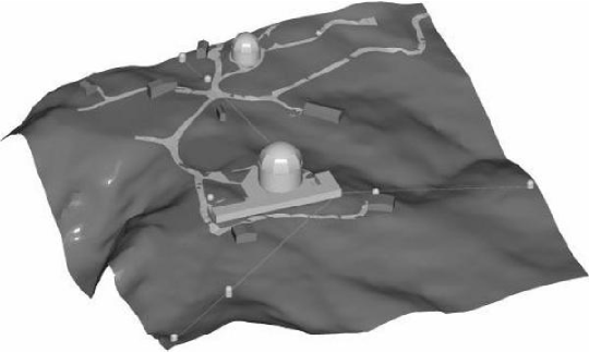
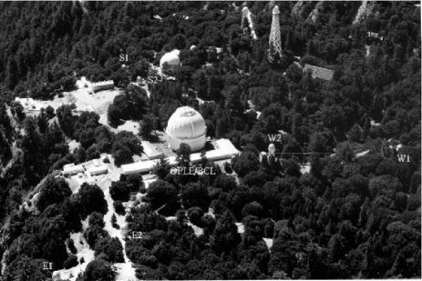
Figure 1: Top: Output of the computer model of the mountain showing the layout of the CHARA Array. This is a view from the north looking south. The 100-in telescope dome is in the center with the L-shaped delay line and beam combining facility building directly behind it. Bottom: A photograph of the site taken from the north looking south. The 100-in dome is clearly visible behind the OPLE/BCL building.

The CHARA Array is built in a non-redundant Y configuration with two telescopes located along each of the three arms of the interferometer. A great deal of attention was paid to having as little impact on the existing structures and trees along the Array arms as possible, and while some road work was required, no existing structures and only a handful of trees had to be removed to fit the Array on the mountain. Figure 1 shows two overviews of the mountain. One is the output of the computer model of the mountain developed early in the project (ten Brummelaar, 1996) to help us position the Array. This model includes all existing roads, buildings and trees and allowed us to experiment with various locations for the telescopes, buildings and light pipes and study their impact on the mountain. The second part of Figure 1 shows a photograph of the actual construction as it was in 2000. All six domes and the central beam synthesis facility are visible in this picture as well as the vacuum light tubes from the east and west arms of the Array.

A list of all available baselines is given in Table 1, and Figure 2 shows the UV coverage for all six telescopes for three hours either side of transit for declinations of $-15^{\circ}$, + $30^{\circ}$ and $+75^{\circ}$.

4 Facilities Overview

There are five primary components to the CHARA facilities on Mount Wilson: the telescopes and telescope enclosures; the vacuum light pipes and their mounting and alignment structures; the central beam synthesis and delay line building; the control room and office building, and a small workshop. Each of these will be discussed in a separate section below, except for the control room and office building which is of standard construction, and the workshop which makes use of an existing building on the mountain that originally served as the delay line and beam combining laboratory for the Mark III Interferometer (Shao et al., 1988).

4.1 Light Collecting Telescopes

Each of the six telescopes is a 1-m Mersenne-type a-focal beam reducer that injects a 12.5-cm output beam into the vacuum transport tubes (Barr et al, 1995). The primary and secondary optics were manufactured as matched sets at LOMO in St. Petersburg, Russia, under a contract with Telescope Engineering Company of Golden, Colorado. The substrates for the 1-m primary and matched secondary are low-CTE Sitall and Zerodur, respectively. The typical primary mirror performance is 0.035 waves rms at 633-nm and because the secondary and primary pairs are matched sets the combined performance of the telescope system exceeds this specification (Bagnuolo, 1996). A seventh matched set has been fabricated for CHARA in St. Petersburg. These optics are an investment toward a future seventh telescope as well as a spare set should delays occur in periodic re-coating of existing optics.

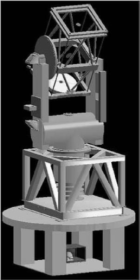
Figure 3: A CAD drawing of the CHARA telescope. The azimuth bearing is at the base of the fork, beneath the cable wrap drums. Friction drive and idler rollers at the azimuth drive disk complete the azimuth drive axis definition. The elevation bearings are at the tops of the fork tubes, as is the elevation drive disk. The entire telescope assembly rests on a concrete pier whose height varies from telescope to telescope in order to provide the correct location above the local terrain. Beneath the telescope lies the coudé box containing mirror #7.

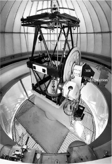
Figure 4: A composite picture of the W1 telescope. The elevation drive system is on the right-hand side of the telescope. To the right of this are the M4 and M5 mounts with the acquisition camera mounted in between. The primary mirror M1 at the bottom of the telescope and the secondary M2 at the top are also visible, as well as the small corner cube in the center of M2. M3 lies in the center with M1 below it. Photograph by Steve Golden.

CHARA commissioned a custom telescope mount design from Mr. Larry Barr. The design is a fork-style alt-azimuth mount with 7 mirror coudé beam extraction. On one side of the fork, the telescope beam is available over several meters in collimated space for acquisition, or future adaptive optics correction. The mounts are exceptionally stiff and massive (23,000 pounds) for interferometric stability, and incorporate an Invar metering truss for temperature insensitive focus. This results in very high stability of the focus of the telescopes which stay in alignment for up to a year without the need for focus adjustment. The primary mirror cell utilizes a central radial support and 18-point whiffle tree, while the secondary support is actuated for adaptive tip/tilt control (ten Brummelaar, 1996). M3 Engineering and Technology Corporation, of Tucson, fabricated and assembled the mounts. A CAD model of the telescope design is given in Figure 3, while Figure 4 shows an actual telescope. Ridgway & McAlister (2003) and Sturmann et al. (2003) give more detailed descriptions of the CHARA telescopes.

Telescope pointing and tracking are controlled using ComSoft TCS supplemented by Tpoints pointing model software to provide typical pointing accuracies of 20 arcseconds rms. A CCD camera located at the Nasmyth port provides for alignment to the central laboratory as well as for the initial acquisition of stars (Sturmann, 1998). The secondary mirror has a small corner cube in the center so that an alignment laser sent out from the laboratory can also be seen in the acquisition system. This ensures that the telescope pointing and laboratory alignment match. Each telescope also has a wide-field finder telescope and several small surveillance cameras to monitor telescope and enclosure status.

The telescope drives are DC servo motors supplied by Parker/Compumotor. These were selected in the hope that they would provide very smooth motion and still behave like stepper motors from a control point of view. In the early commissioning of the telescopes the drives were found to have a small, sub-hertz oscillation, which we had originally thought to be caused by the mechanical design. After a re-design of these drives we found that the oscillation was still there. It was later discovered to be caused by poor tuning of the servo system for the drive motors, and we reverted to the original mechanical design.

Attached to the telescopes themselves is a custom CHARA designed and built telescope control system called the “TElescope MAnager” (TEMA). TEMA controls all the various telescope covers, cameras, and alignment jigs in the dome as well as providing a local interface to the telescope control software. A local control pad and hand paddle allow an operator to control the telescope and dome from within the enclosure, as well as remotely adjust mirrors in the beam synthesis laboratory to align the optical delay beam axis to the telescope beam axis.

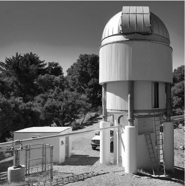
Figure 5: The E2 telescope enclosure and electronics bunker. The small entry door can be seen on the right of the lower cylinder. Both the upper and lower cylinders can move to allow a free flow of air around the telescope. The light pipe from E1 comes from the left, passes through the coudè area below the lower cylinder and leaves to the right with the light pipe from E2. Photograph by Steve Golden.

The telescopes are mounted on massive pedestals with a coudé area below where the extracted beam is polarization compensated and directed to the central laboratory. The surrounding enclosures are structurally independent of the telescope pedestals, with lower and upper rings supporting a pair of nested cylinder walls which open top and bottom for access and ventilation. The walls provide $360^{\circ}$ free flow of air, which is successful in suppressing dome seeing in spite of the very low wind speed conditions typical at Mount Wilson. The telescope enclosures incorporate 16.5-ft domes (provided by Ash Manufacturing with extra wide slits) slaved to the telescope azimuth. CHARA’s prime contractor on Mt. Wilson, Sea West Corporation, of San Dimas, California, suggested this novel concentric cylinder design. All enclosure and telescope functions are remotely operable (Hines & ten Brummelaar, 2002), and all telescope and enclosure control electronics, except TEMA are located in adjacent cement block bunkers to avoid heat production within the enclosures. Figure 5 shows the enclosure and electronics bunker for the E2 telescope.

All six telescopes are in place with all telescope optics installed and aligned, and all telescopes are in regular interferometric operation. It is not necessary to visit the telescopes themselves under normal conditions to align, operate and close down the Array. The last telescope to be commissioned in interferometric mode came on line in November 2003, and subsequently the Array has been observing nightly.

4.2 Vacuum Light Beam Transport Tube

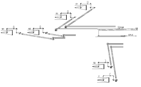
Figure 6: Schematic of the optical train bringing the light from each telescope to inside the beam synthesis facility. Full optical symmetry has been maintained despite the three-dimensional nature of the mountain layout.

Seven reflections are required to direct the output beam from each telescope to the central beam combination facility, with mirror #7 housed in the coudé box beneath the telescope. In order to preserve polarization symmetry around the three arms of the Y-array, one or two additional mirrors, depending upon the Array arm, are housed in this box. Figure 6 shows the layout of these relay mirrors. These extra reflections are required because of the three-dimensional nature of the layout on the mountain. In this way optical symmetry is maintained in all arms of the interferometer (Traub, 1988; Ridgway, 2004). We have found no evidence for anomalous polarization effects in the data on the sky. The coudé optics inject the light through an optical window into a vacuum tube for transport to the Array center. Aluminum tubing with an outside diameter of 20-cm accommodates the 12.5-cm light beams. Neoprene sleeves join thirty-foot lengths of this tubing, a technique that was first used by Michelson in his speed of light experiments on Mount Wilson and is also effectively used at other interferometers.

Each telescope has a dedicated vacuum tube (Ridgway et al., 2000) so that each arm of the CHARA Array feeds two parallel tubes to the center. The terrain is such that the tubes must be elevated in places by up to 10-m above local ground level. Vertical support posts accommodate alignment and thermal expansion. Vacuum operation is not required for interferometric measurements in the near infra-red bands, but does provide better image quality, especially in the early part of the night. Since mid-2004, all night-time operation takes place with the system under vacuum. The vacuum pump is vibration isolated and it is possible to run the pump while observing and keep the vacuum at 0.5-Torr or lower throughout the night.

4.3 Central Beam Synthesis and Delay Line Building

The delay lines, beam management subsystems, and beam combination subsystems are all housed in the central “beam synthesis facility” (BSF), an L-shaped building whose 94-m longest dimension houses the delay lines while the short part of the “L” comprises the “beam combination laboratory” (BCL). The BSF is a “building within a building” where the envelope between the inner and outer buildings serves as a heating and air conditioning plenum. This keeps the 1,000-m² of laboratory space at a reasonably constant and uniform temperature. The foundations and footings of the inner and outer structures are not structurally connected to minimize vibration transmission, and 24-inch thick concrete slabs beneath the optical tables and rail supports provide stability to interferometric tolerances for all optical components.

4.3.1 Optical Path Length Compensation

Maintenance of zero optical path length difference is a major overhead for an optical interferometer with baselines of hundreds of meters. This is accomplished at the CHARA Array in two stages in an over-and-under arrangement. The first stage occurs while still in vacuum with six parallel tube systems (referred to as the “Pipes of Pan” or PoP’s) (Ridgway, 1994) having assemblies with fixed delay intervals of 0-m, 36.6-m, 73.2-m, 109.7-m and 143.1-m, that feed a mirror into the beam to reflect it back toward a periscope system that brings the beam into the continuous part of the delay system. Incoming beams from the three arms of the Array are fed into the parallel PoP tubes by mirrors in large “turning boxes” that also serve to complete the polarization symmetry requirement. Down each PoP line are mirrors that can be moved into the beam to add, or remove, fixed amounts of delay. At the end of each PoP line is a stationary “end” mirror that represents the longest possible static delay available in the system. Upon exiting the PoP’s, beams leave vacuum and are injected into the continuous delay lines by a pair of periscope mirrors.

The continuously variable delay is provided by the “optical path length equalizers” (OPLE’s), a mid-generation design provided to CHARA under a contract with JPL in the evolutionary chain from the Mark III Interferometer to the Keck Interferometer (Colavita et al., 2004). The OPLE’s are not in the vacuum system and incorporate a cats eye arrangement in which an incoming beam reflects off one side of a parabola, comes to focus on a small secondary, returns to the other side of the parabola and then, re-collimated, is fed back parallel to the incoming beam. Each cart rides on precision-aligned cylindrical steel rail pairs 46-m in length. A four-tiered nested servo system, with feedback from a laser metrology unit, provides 92-m of path length compensation tracking with an rms error of better than 20-nm, and typically as good as 10-nm. All 24 PoPs, six end mirrors, and all six OPLE carts are installed and are fully operational.

4.3.2 Beam Management

Following path length compensation in the PoP/OPLE subsystems, the emerging 12.5-cm beams of light are reduced to a final diameter of 1.9-cm using a two-element “beam-reducing telescope” (BRT). The reduced beams then pass through the “longitudinal dispersion corrector” (LDC) subsystem that corrects for the difference in air paths between two beams arising from the fact that the telescopes are not at the same elevation and that part of the optical path is not in vacuum (Berger, 2004; Berger, ten Brummelaar, Bagnuolo, & McAlister, 2003). The “beam sampling system” (BSS) provides the final stage of beam management. The BSS uses a dichroic beam-splitter and a flat mirror to separate visible from infrared light at the 1-$\mu$m boundary and then turns the two beams through 90^∘ and sends them along parallel paths to the visible and IR beam combiners. Each BSS assembly is movable on a precision stage so that it also serves as a switch yard for selecting baseline pairs to be directed to the beam combiners.

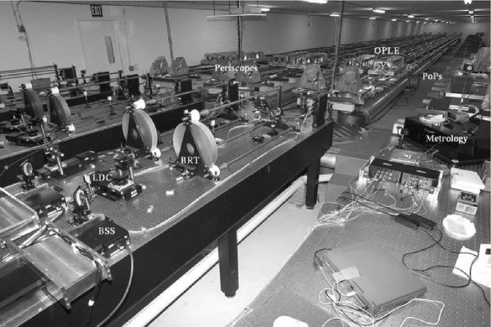
Figure 7: The delay line and beam management area. The PoPs, Periscopes, OPLEs, BRTs, LDCs and BSS system are clearly visible. Photograph by Steve Golden.

As with most subsystems in the Array, we are continually working to improve the beam management system. Nevertheless, all six beam trains are complete and operational and all telescopes and beam trains have been used for interferometry and are available for science. Figure 7 shows a picture of the delay line and beam management area.

4.3.3 Beam Combination

The BCL currently houses five optical tables based upon functionality of subsystems. These tables contain the visible beam combiner, the infrared beam combiner, a HeNe laser for bore sighting/alignment and a white-light source for internal fringe generation, detectors for fringe and tip/tilt tracking, and a fiber-based beam combiner (Coudé du Foresto et al., 1997; Coude du Foresto et al., 2003) resulting from a collaboration with the Paris Observatory.

At the time of writing, all beam combination in the CHARA Array has been restricted to two-beam systems. Future upgrades in 2005 will include a three-way open-air beam combiner capable of measuring three baselines and a single closure phase. The tests are already underway of a four- to six-way fiber-based beam combiner being designed and constructed by Dr. John Monnier at the University of Michigan (Monnier, 2004). In late 2004, a new grant from the National Science Foundation was awarded to Dr. Monnier and collaborators at Georgia State University and the Michelson Science Center to fund a six-way IR-band fringe tracker. We expect the detailed design and construction of this system to begin in 2005.

It was decided early on in the design phase of the CHARA Array to separate the functions of fringe tracking and fringe amplitude and phase measurement (ten Brummelaar & Bagnuolo, 1994). In this way, each system can be optimized for one task or another and development of the various beam combiners can go on in parallel. We are exploring several methods of fringe tracking, including packet tracking where one keeps the fringe packet centered in a long scan, group delay tracking where one keeps the center of the group delay in position, and phase locking where one tracks on a single fringe. It is expected that all three methods will be used under different conditions and for different science targets. For example, it will be possible to phase lock using the IR system and send a phased beam into the visible beam combiner. The reverse will, of course, also be possible. It will even be possible to divide the six telescopes between several beam combiners and thereby create separate interferometers working in parallel.

Two high-speed CCDs have been purchased from Astronomical Research Cameras of San Diego for use in the visible beam combination area, one for the I and R band beam combiner and one for tip/tilt detection. We have also acquired a fiber coupling stage that breaks the full aperture into seven smaller apertures and couples each of these to a multi-mode fiber. The central beam includes the telescope secondary obscuration and is therefore used primarily for alignment. This allows us to have seven small (30-cm on the sky) aperture systems feeding a fiber-based slit in the low resolution spectrograph and process all seven systems in parallel (Ogden, ten Brummelaar, & Sturmann, 2003). The construction of this visible light system is in progress, and we expect to have achieved first fringe on the sky by late 2004.

A higher spectral resolution spectrograph is also under construction and will use the same sub-apertures and fibers (Hillwig, Bagnuolo, & Riddle, 2002). This spectrograph is intended for combined high spatial and high spectral resolution measurements. The spectrograph is a modified Ebert-Newtonian based on the design used for the Georgia State Multi-Telescope Telescope (Barry, Bagnuolo, & Gies, 1994). It is fiber-fed and will produce coherent, spatially resolved spectra. The use of this spectrograph on the sky is delayed until phase locking is possible at the CHARA Array so that phased beams can be sent into the system. This should be possible in late 2005.

The second camera is being tested as a tip/tilt detection upgrade. In lieu of a full-up visible light beam combiner, the visible channel short of 600-nm is presently used entirely for photomultiplier based tip/tilt detection for which the high bandwidth limiting magnitude is V = +9.5 at 10-ms sample times, although in good seeing conditions that permit the use of longer integration times, we can track objects as faint as V = +12.0. This tip/tilt detection scheme and correction algorithm is largely based on the system developed at the Sydney University Stellar Interferometer (SUSI) (ten Brummelaar & Tango, 1994). Light from 600-nm to 1-$\mu$m is divided between an intensified CCD, allowing for image quality inspection and alignment, and the low-resolution spectrograph used for I and R band interferometry. The bore sight laser and white light sources are regularly used for the essential tasks of alignment and overall system fine-tuning. The ICCD also supplies us with a reference position defining the optical axis of the interferometer, and we regularly align the tip/tilt detectors to ensure that star images from each telescope lie on this optical axis.

The layout of the current IR beam combiner, dubbed “CHARA Classic”, is that of a simple pupil-plane beam combiner (Sturmann et al., 2003). The two outputs from the beam splitter are separately imaged onto two spots on the beam combiner camera (described below), with fringes detected in a scanning mode provided by dithering a mirror mounted to a piezoelectric translation stage. The stage is driven with a symmetric saw tooth signal whose response to a given driving signal was mapped with a laser interferometer to provide a 1-kHz data acquisition rate corresponding to five samples per fringe at a typical 200 Hz fringe frequency. Sample rates of 250, 500 and 750 Hz are also possible. The current K limiting magnitude for fringe detection with this system is K = +6.5 for raw visibilities of 0.50.

This system is also capable of IR phase locking, which has successfully been achieved in the lab, with the goal of the system working on starlight in 2005. This will improve throughput from one sample every 0.5 sec to 80 samples/sec and ultimately provide the ability to fringe track in H band with CHARA Classic and gain several magnitudes in K band using the fiber based beam combiner described below. It will also be possible to phase lock in one of the IR bands in order to provide phased beams for both the low- and high-resolution visible spectrographs.

In our current fringe scanning method the maximum sample time is 4-ms, however, with the new phase locking method it is possible to increase this to 20-ms or more. Furthermore, all mirror surfaces are currently coated with Al, and the remaining project funding provides for upgrading a number of relay mirrors in vacuum or in sheltered environments with over-coated silver. Our calculations show (Ridgway, 2004) that silver coatings will double the near IR throughput and the expected gain in the visible red is much larger. These and other steps are expected to increase sensitivity to K = +9.0.

Through a collaboration with the Paris Observatory, a second beam combiner has been installed at the CHARA Array. The Fiber-Linked Unit for Optical Recombination (FLUOR) has been in use at the IOTA interferometer on Mt. Hopkins since 1995 (e.g. Perrin et al. (1999)). The special feature of FLUOR is that it incorporates optical fibers as spatial filters and a fiber X junction as the interfering element instead of a beam splitter. The combination of spatial filtering with subsequent photometric monitoring of beam intensities permits this instrument to measure visibilities of bright objects with precisions of better than 1%. FLUOR is a key tool for problems such as accurate measurement of variable star pulsation, stellar shapes for main sequence and pre-main sequence stars, large $\Delta$m binaries, and limb darkening determination through measurements beyond the first null in visibility that require such high accuracies. The FLUOR beam combiner has been used regularly on the sky since early 2003.

4.3.4 IR Beam combiner camera

The heart of the infrared beam combiner is a Rockwell 256$\times$256 HgCdTe PICNIC array with 40-$\mu$m pixels possessing QE’s better than 60% in the 1 to 2.3-$\mu$m spectral regime. The CHARA “Near Infrared Observer” (NIRO) camera was built at Georgia State with the kind assistance of Drs. Wes Traub and Rafael Millan-Gabet of the Harvard-Smithsonian Center for Astrophysics. NIRO is thus very similar to the camera used at the IOTA interferometer (Millan-Gabet, Schloerb, Traub, & Carleton, 1999; Pedretti et al., 2004).

The PICNIC array is sensitive to light at wavelengths of 0.8 to 2.5-$\mu$m and is electrically structured as four 128$\times$128 quadrants, each with its own output amplifier; NIRO is wired to read out only one quadrant. Array control and data acquisition are controlled by a digital I/O board in a PC and a custom-built interface box containing a clock driver board that provides the DC bias levels for the array and an analog-to-digital converter (ADC) board. The input to the ADC board is the array’s analog output signal, buffered by a low-noise 20$\times$ pre-amplifier mounted on the inside of the dewar lid (operating near room temperature). The ADC is a 16-bit unit capable of 100 kilo-samples per second.

The PICNIC array is mounted in an Infrared Laboratories HDL-5 dewar modified for use with liquid nitrogen in both cryogen cans. Vacuum in the dewar is maintained to better than 10^-8-Torr by a combination of molecular sieves and an ion pump, resulting in a dewar hold-time of 22 hours. A 60^∘ off-axis parabolic mirror focuses the two collimated interferometer beams into two spots on the array after passing through a fused silica vacuum window and a cooled filter. The filter wheel can be rotated manually and holds up to six filters. Currently, it holds H and K^′-band filters, as well as several narrow-band filters within the K band.

5 Control System

The Array control system is based upon real-time Linux except for the OPLE subsystem, which was developed by JPL and runs under VxWorks, and the FLUOR beam combiner, which utilizes Labview. The control system is fully operational although it is subject to frequent updates and improvements as observing experience is gained.

The control model consists of several layers. At the lowest level is the real-time code which is slaved to a 1-ms clock tick derived from GPS and distributed around the entire Array. In this way we can run synchronous tasks across many CPUs distributed throughout the facility. In the second layer, each real-time process is controlled by a server program run in the Linux environment. This server provides a command line interface that provides full control of the system in question as well as many engineering test routines and functions. Each server can be logged into remotely via a simple text-base interface for remote engineering and test operations. At the highest level, more user-friendly GUI programs based on the GTK windowing system can connect via a TCP/IP socket to any server and provide all the functionality normally required for observing. Sequencing is done by a single client program, dubbed the “Central Scrutinizer”, that connects to all servers and controls the acquisition of stars, data collection and writing a log of all activity. Acquiring a new target consists of entering an HD, SAO or IRC number and clicking a single button. The Central Scrutinizer also automatically collects baseline solution and telescope pointing data.

Because of the client/server model used, the CHARA Array can be controlled from a single remote CPU via a secured internet connection and this accessibility has been utilized to establish the Cleon C. Arrington Remote Operations Center (AROC), located in Atlanta on the Georgia State campus. A second remote control facility has been established on the grounds of the Paris Observatory and was used to control the Array for the first time in June of 2004. A remote capability for the FLUOR beam combiner was added in late 2004 (Mérand et al, 2004).

An IDL-based observing planning tool for CHARA has been developed (Aufdenberg,, 2004) that provides a complete tool set for planning observations with the CHARA Array: providing UV coverage plots; times when a particular object is available for observation; theoretical visibility plots; and aids in the selection of telescope and PoP configurations. This planning tool can be downloaded at http://www.noao.edu/staff/aufdenberg/chara_plan.

6 Data Processing

While we fully expect our views and methods on data analysis to evolve with time we will discuss here the two methods currently in use at the CHARA Array. Both are based on the work of Benson, Dyck, & Howell (1995) and yield results consistent with one another, though the second method is more reliable in low signal to noise data.

We write the fringe signal on each detector pixel as

$$D_{i}(t)=\frac{I_{i1}+I_{i2}}{2}+\,(-1)^{i}\,\sqrt{I_{i1}I_{i2}}\,\nu\,{\rm sinc}(\pi\,\Delta\sigma\,v_{g}t)\cos(2\pi\sigma_{0}v_{g}t+\phi)$$ (1)

where $I_{ij}$ is the light intensity that reaches detector $i$ from telescope $j$, $\nu=V\times V_{\rm sys}$ is the correlation of the two beams related to the visibility of the object $V$ and the system visibility $V_{\rm sys}$, the optical filters are centered at wave number $\sigma_{0}$ and have a band pass of $\Delta\sigma$, $v_{g}$ is the group velocity of the fringe packet resulting from the motion of the dither mirror, and $\phi$ is the sum of the fringe phase and the atmospherically induced phase error.

This must be calibrated for beam intensity, so this expression is normalized using a low-pass filtered version of itself resulting in

$$N_{i}(t)=1+\,(-1)^{i}\,\frac{2\sqrt{I_{i1}I_{i2}}}{I_{i1}+I_{i2}}\,\nu\,{\rm sinc}(\pi\,\Delta\sigma\,v_{g}t)\cos(2\pi\sigma_{0}v_{g}t+\phi)$$ (2)

where instead of intensities we now have the normalized signal $N_{i}(t)$ and we see that there will be a transfer function due to the light intensities for each detector channel given by

$$T_{i}=\frac{2\sqrt{I_{i1}I_{i2}}}{I_{i1}+I_{i2}}.$$ (3)

In the first data reduction method used at the CHARA Array, we put the normalized signal $N_{i}(t)$ through a bandpass filter centered at the frequency expected due to the dither mirror motion. An example processed fringe, from the rapidly rotating star Regulus (HD 87901) observed on 16 April 2004 with the E1-S2 baseline, is shown in Figure 8. The top frame shows the raw fringe with the smoothed version of that fringe, obtained from the low-pass filtering, superimposed. The middle frame (shifted by 0.2 in relative intensity for clarity) is that fringe normalized to the smoothed version, and the bottom frame is the result of bandpass filtering after which the maximum absolute excursion from zero relative intensity is a measure of $\nu$. These fringes exhibit symptoms of longitudinal dispersion, which will be corrected by the LDC system mentioned previously. For most high signal to noise cases this analysis method works well, though it has a tendency to overestimate the correlation for low signal to noise data.

A second method of analysis is based on a spectral analysis. If we compute the power spectrum of the fringe signal we get

$${\rm PS}\left[N_{i}(t)-1\right]=T_{i}^{2}\left[\frac{\nu}{\Delta\sigma\,v_{g}}\right]^{2}\left[\Pi\left(\frac{\nu-\sigma_{0}v_{g}}{\Delta\sigma\,v_{g}}\right)+\Pi\left(\frac{\nu+\sigma_{0}v_{g}}{\Delta\sigma\,v_{g}}\right)\right]$$ (4)

where

$$\Pi(x)=\left\{\begin{array}[]{ll}0,&|x|>\frac{1}{2}\\ \frac{1}{2},&|x|=\frac{1}{2}\\ 1,&|x|<\frac{1}{2}\\ \end{array}\right.$$ (5)

and since the fringe signal is a real signal, we can safely ignore the negative spatial frequencies and write

$${\rm PS}\left[N_{i}(t)-1\right]=T_{i}^{2}\left[\frac{\nu}{\Delta\sigma\,v_{g}}\right]^{2}\Pi\left(\frac{\nu-\sigma_{0}v_{g}}{\Delta\,\sigma v_{g}}\right).$$ (6)

The total integral of the power is then

$$S_{i}=\int d\nu\,{\rm PS}\left[N_{i}(t)-1\right]=T_{i}^{2}\frac{\nu^{2}}{\Delta\sigma\,v_{g}}$$ (7)

and this results in an estimate of $\nu^{2}$.

Since there will also be detector, scintillation and photon noise in the signal, these must be removed before the final integration is performed. Each data set is followed by a series of data scans incorporating shutters to provide data from each telescope separately and without light from either telescope. The power spectrum with both shutters closed contains only detector noise, while those with light from the telescopes contain detector noise as well as half the scintillation and photon noise. This contains enough information to remove the noise bias as well as to estimate the transfer function $T_{i}$. An example power spectrum of a fringe signal taken of the star HD 138852 on June 6th 2004 is given in Figure 9.

There is one more correction that can be made to the correlation estimate. Because of atmospheric turbulence, the correlation is changing constantly and so can be considered to be a random variable with some mean $\overline{\nu}$ and a variance $\sigma_{\nu}^{2}$. Since we are measuring the mean of the square of the correlation, we are actually measuring

$$\overline{\nu^{2}}=\overline{\nu}^{2}+\sigma_{\nu}^{2},$$ (8)

and thus all estimates of the square of the correlation are biased by the variance of the correlation. Unfortunately, it is not possible to take the square root of $S_{i}$ as, due to the statistical nature of the measure, it is sometimes negative. It is, however, possible to square $S_{i}$, resulting in an estimate of $\overline{\nu^{4}}$. If one assumes the statistical distribution of the correlation is normal, one can then form the unbiased estimator for the correlation

$$\overline{\nu}=\left(\frac{3\overline{\nu^{2}}^{2}-\overline{\nu^{4}}}{2}\right)^{\frac{1}{4}}$$ (9)

with the corresponding variance estimate

$$\sigma_{\nu}^{2}=\sqrt{\overline{\nu}^{4}-\frac{1}{2}(\overline{\nu^{2}}^{2}-\overline{\nu^{4}})}-\overline{\nu}^{2}.$$ (10)

Since the real correlation can never be negative, it is sometimes better to use a log-normal distribution, normally parametrized using the variables $\mu$ and $\sigma^{2}$. These can be determined using

$$\mu=\frac{1}{4}\ln\frac{\overline{\nu^{2}}^{4}}{\overline{\nu^{4}}}$$ (11)

and

$$\sigma^{2}=\frac{1}{4}\ln\frac{\overline{\nu^{4}}}{\overline{\nu^{2}}^{2}}$$ (12)

from which we get the unbiased correlation estimate

$$\overline{\nu}=\exp(\mu+\frac{1}{2}\sigma^{2})$$ (13)

with the variance

$$\sigma_{\nu}^{2}=\exp(2\mu+2\sigma^{2})-\exp(2\mu+\sigma^{2}).$$ (14)

In practice the normal and log-normal equations give virtually the same results during times of good seeing, or high correlation, and typically fail at very low signal to noise. An example of some raw correlation data is given in Figure 10. In this figure histograms of the raw correlation measured during two separate measurement sequences are shown for the same object, one taken during a time when the seeing was approximately 1 arcsecond and one when the seeing was approximately 2 arcseconds. Superimposed on these plots are the best fit Gaussian curves. In the case of good seeing the histogram is very symmetric and well approximated by a normal distribution, whereas the histogram made during poor seeing is very asymmetric and a log-normal distribution is required.

The effect of the correlation bias discussed above is also quite clear in these data. In the reduction of the data taken during good seeing the correlation estimates based directly on equation (7) is $0.542\pm 0.110$, where the error quoted here is the formal standard deviation of the measurement, while those based on the de-biased estimates in equation (9) and (13) are $0.542\pm 0.185$ and $0.543\pm 0.100$ respectively. All three measures agree. On the other hand, these estimators produced $0.180\pm 0.091$, $0.145\pm 0.165$ and $0.172\pm 0.084$ in the poor seeing example, a difference of 8%. Clearly, this measurment bias is very important unless the conditions and instrument performance are both very good.

This bias due to correlation variance is not significant in fiber based beam combiners such as FLUOR due to the spatial filtering of the beams, and will also be much less important in smaller aperture interferometers. Still, in the case of CHARA’s larger apertures is certainly does affect the final calibrated result, and our investigation of this correlation bias process continues.

A typical dataset for a target star is a sequence of scans in which the target is interleaved between scans of a reference or calibrator star that has been selected on the basis of having a well-known visibility or an expected visibility near unity. Time variations in instrumental visibility due to seeing and other effects are compensated for by interpolating the target epochs to the calibrator epochs and then dividing the measured correlations by the interpolated calibrator visibilities corrected for the expected calibrator visibility. Software has also been written to enable us to use the output of this analysis and put it in the correct format for use with the calibration and data reduction software produced by the Michelson Science Center (Boden, Colavita, van Belle, & Shao, 1998).

Figure 11 shows two complete measurement sets taken from the same two nights as shown in Figure 10. The projection angle on the object was different on these two nights so one expects a change in the object visibility, indeed the actual object visibility was higher during the night of poor seeing than during the night of good seeing. Still, the calibrator raw correlation changes significantly in poor seeing and remains fairly stable in good seeing. The bottom line in interferometry is calibration of the data and the biggest impact on this is the seeing. Despite our efforts to de-bias our correlation estimators, the formal errors found in the measurement process are always smaller than those created by the calibration process. Our best efforts during the observing season of 2004 resulted in calibrations good to 4% when using the open air beam combiner without spatial filtering. This is reduced to better than 1% when using the fiber based combiner and spatial filtering.

As of this writing, more than 5000 data sets have been collected from 12 baseline pairs since late 1999. The majority of the early observations have been for engineering purposes, and it has only been since the spring of 2002 that the observing has been directed toward science rather than engineering. The first full year of observing directed primarily toward science observations was 2004. In that year we opened the telescope domes on a total of 229 nights, and of those nights we collected useful data on 154 nights. While seeing clearly affects our ability to calibrate the data we have found it is still possible to collect data until the correlation length $r_{0}$ falls below 3cm. Below this it is still possible to obtain fringes, though it is all but impossible to achieve any sort of worthwhile calibration. No strong correlations between data quality and time of night have been found, though we have found four distinct observing seasons here on Mount Wilson. During the winter, the seeing is poor and we are frequently closed due to high winds, rain or snow. Conditions improve during the spring and our best season occurs during the summer months where we often have many clear nights of excellent seeing in a row. The fall season is similar to the spring, though often affected by high winds.

7 Conclusion

The full-time science program of the CHARA Array has been underway for only a year, and we expect many exciting years of science, technical development and data analysis exploration to come. The CHARA Array was built within the original budget and on a reasonable time line by a small university-based group of scientists. Many lessons have been learned along the way from the earliest days of CHARA that might be valuable to future projects, and so we plan to describe that experience in another venue.

All six telescopes, light pipes, delay lines, beam reducers, longitudinal dispersion correctors and beam sampling systems are installed and fully operational, and the Array is now regularly scheduled for a variety of astronomical projects. While routine science observing is underway, we look forward to continual technical and performance improvements including such capabilities as phase closure and multi-way beam combination expected to begin in 2005.

Table 1: Available baselines. These numbers are based on the results of a global baseline solution from mid-2004. The RMS error of this fitting process was 1891-$\mu$m.

Telescopes	East (m)	North (m)	Height (m)	Baseline (m)
S2-S1	-5.748	33.581	0.644	34.076
E2-E1	-54.970	-36.246	3.077	65.917
W2-W1	105.990	-16.979	11.272	107.932
W2-E2	-139.481	-70.372	3.241	156.262
W2-S2	-63.331	165.764	-0.190	177.450
W2-S1	-69.080	199.345	0.454	210.976
W2-E1	-194.451	-106.618	6.318	221.853
E2-S2	76.149	236.135	-3.432	248.134
W1-S2	-169.322	182.743	-11.462	249.392
W1-E2	-245.471	-53.393	-8.031	251.340
W1-S1	-175.071	216.324	-10.818	278.501
E2-S1	70.401	269.717	-2.788	278.767
E1-S2	131.120	272.382	-6.508	302.368
W1-E1	-300.442	-89.639	-4.954	313.568
E1-S1	125.371	305.963	-5.865	330.705

Figure 2: UV coverage of the CHARA Array for declinations -15^∘ (top left), +30^∘ (top right) and +75^∘ (bottom). Each plot shows the coverage resulting from all six telescopes within three hours either side of transit. The units have been left in meters due to the wide range of possible wavebands in use at CHARA.

Figure 8: A fringe scan is shown above in its raw signal form (top) with the low-pass filtered version superimposed prior to normalization. The bottom frame shows the same scan, with an offset of 0.2 for clarity, after normalization and, finally, after implementation of the band-pass filter.

Figure 9: An example of a raw power spectrum (top) showing a combination of the fringe signal, photon noise, scintillation noise and camera noise. Once the noise has been measured and removed only the fringe signal remains (bottom).

Figure 10: Two histograms of raw correlation as measured on the same object HD 197373 on two different nights, one of good seeing 2004-06-20 (solid line) and one of poor seeing 2004-06-29 (dashed line). The actual correlation at both times should be close to unity. The dotted lines show the best fit Gaussian curve for each data set.

Figure 11: Two examples of a complete measurement sequence using the calibrator HD 197373 (squares) and the object HD 203280 (triangles) on a night of good seeing (top) and a night of poor seeing (bottom). These data are from the same two nights as those shown in Figure 10.

References

- Aufdenberg, (2004) Aufdenberg, J. P. 2004, CHARA Technical Report #90, http://www.chara.gsu.edu/CHARA/techreport.html/TR90.pdf
- Bagnuolo (1996) Bagnuolo, W.G. Jr. 1996, CHARA Technical Report #37, http://www.chara.gsu.edu/CHARA/techreport.html/TR37.pdf
- Barr et al (1995) Barr, L., Gerzoff, A., & Ridgway, S. T. 1995, CHARA Technical Report #9, http://www.chara.gsu.edu/CHARA/techreport.html/TR9.pdf
- Barry, Bagnuolo, & Gies (1994) Barry, D. J., Bagnuolo, W. G. Jr., & Gies, D. R. 1994, Bulletin of the American Astronomical Society, 27, 760
- Benson, Dyck, & Howell (1995) Benson, J. A., Dyck, H. M., & Howell, R. R. 1995, Appl. Opt., 34, 51
- Berger (2004) Berger, D. H. 2004, PASP, 116, 390
- Berger, ten Brummelaar, Bagnuolo, & McAlister (2003) Berger, D. H., ten Brummelaar, T. A., Bagnuolo, W. G. Jr., & McAlister, H. A. 2003, Proc. SPIE, 4838, 974
- Boden, Colavita, van Belle, & Shao (1998) Boden, A. F., Colavita, M. M., van Belle, G. T., & Shao, M. 1998, Proc. SPIE, 3350, 872
- ten Brummelaar & Tango (1994) ten Brummelaar, T. A. & Tango, W. J. 1994, Experimental Astronomy, 4, 297
- ten Brummelaar & Bagnuolo (1994) ten Brummelaar, T. & Bagnuolo, W. G. Jr. 1994, Proc. SPIE, 2200, 140
- ten Brummelaar (1996) ten Brummelaar, T. A. 1996, CHARA Technical Report #39, http://www.chara.gsu.edu/CHARA/techreport.html/TR39.pdf
- ten Brummelaar (1996) ten Brummelaar, T. A. 1996, CHARA Technical Report #48, http://www.chara.gsu.edu/CHARA/techreport.html/TR48.pdf
- ten Brummelaar et al. (2000) ten Brummelaar, T. A., Bagnuolo, W. G. Jr., McAlister, H. A., Ridgway, S. T., Sturmann, L., Sturmann, J., & Turner, N. H. 2000, Proc. SPIE, 4006, 564
- ten Brummelaar et al. (2003) ten Brummelaar, T. A., McAlister, H. A., Ridgway, S. T., Turner, N. H., Sturmann, L., Sturmann, J., Bagnuolo, W. G. Jr., & Shure, M. A. 2003, Proc. SPIE, 4838, 69
- Buscher (1993) Buscher, D. F. 1993, Bulletin of the American Astronomical Society, 25, 1306
- Buscher (1994) Buscher, D. F. 1994, Proc. SPIE, 2200, 260
- Colavita et al. (2004) Colavita, M. M., Wizinowich, P. L., & Akeson, R. L. 2004, Proc. SPIE, 5491, 454
- Coudé du Foresto et al. (1997) Coudé du Foresto, V., Perrin, G., Mariotti, J., Lacasse, M., & Traub, W. 1997, Integrated Optics for Astronomical Interferometry, 115
- Coude du Foresto et al. (2003) Coude du Foresto, V., et al. 2003, Proc. SPIE, 4838, 280
- Fallon, McAlister, & ten Brummelaar (2003) Fallon, T., McAlister, H. A., & ten Brummelaar, T. A. 2003, Proc. SPIE, 4838, 1193
- Hale et al. (2000) Hale, D. D. S., et al. 2000, ApJ, 537, 998
- Hillwig, Bagnuolo, & Riddle (2002) Hillwig, T. C., Bagnuolo, W. G. Jr., & Riddle, R. L. 2002, Bulletin of the American Astronomical Society, 34, 1130
- Hines & ten Brummelaar (2002) Hines, B. E. & ten Brummelaar, T. A. 2002, Proc. SPIE, 4848, 187
- McAlister et al. (2004) McAlister, H. A., ten Brummelaar, T. A., Aufdenberg, J. P., Bagnuolo, W. G. Jr., Berger, D. H., Coudé du Foresto, V., Mérand, A., Ogden, C., Ridgway, S. T., Sturmann, J., Sturmann, L., Taylor, S. F. 2005, Proc. SPIE, 5491, 472
- (25) McAlister, H. A., ten Brummelaar, T. A., Bagnuolo, W. G. Jr., Berger, D. H., Gies, D. R., Huang, W., Shure, M. A., Sturmann, J., Sturmann, L., Turner, N., Taylor, S., Ogden, C., Ridgway, S. T. & van Belle, G. 2005, ApJ, in press.
- Mérand et al (2004) Mérand, A, Birlan, M., Lelu de Brach, R. & Coudé du Foresto, V, 2004, Proc. SPIE, 5491, 1661
- Millan-Gabet, Schloerb, Traub, & Carleton (1999) Millan-Gabet, R., Schloerb, F. P., Traub, W. A., & Carleton, N. P. 1999, PASP, 111, 238
- Monnier (2004) Monnier, J. D, Berger, J, P, Millan-Gabet, R, & ten Brummelaar, T. A. 2004, Proc. SPIE, 5491, 1370
- Ogden, ten Brummelaar, & Sturmann (2003) Ogden, C. E., ten Brummelaar, T. A., & Sturmann, J. 2003, Proc. SPIE, 4838, 964
- Pedretti et al. (2004) Pedretti, E., et al. 2004, PASP, 116, 377
- Perrin et al. (1999) Perrin, G., Coudé du Foresto, V., Ridgway, S. T., Mennesson, B., Ruilier, C., Mariotti, J.-M., Traub, W. A., & Lacasse, M. G. 1999, A&A, 345, 221
- Ridgway et al. (2000) Ridgway, S. T., et al. 2000, Proc. SPIE, 4006, 696
- Ridgway & McAlister (2003) Ridgway, S. T. & McAlister, H. A. 2003, in SMALL TELESCOPES IN THE NEW MILLENNIUM II. TELESCOPES WE USE, ed. T. Oswalts, Kluwer, pp. 231-254
- Ridgway (1994) Ridgway, S. T., ten Brummelaar, T. A., & Bagnuolo, W, G. Jr. 1994, CHARA Technical Report #4, http://www.chara.gsu.edu/CHARA/techreport.html/TR4.pdf
- Ridgway (2004) Ridgway, S. T., & Bagnuolo, W. G. Jr. 1996, CHARA Technical Report #91, http://www.chara.gsu.edu/CHARA/techreport.html/TR28.pdf
- Ridgway (2004) Ridgway, S. T. 2004, CHARA Technical Report #91, http://www.chara.gsu.edu/CHARA/techreport.html/TR91.pdf
- Shao et al. (1988) Shao, M., Colavita, M. M., Hines, B. E., Staelin, D. H., & Hutter, D. J. 1988, A&A, 193, 357
- Sturmann et al. (2003) Sturmann, J., ten Brummelaar, T. A., Ridgway, S. T., Shure, M. A., Safizadeh, N., Sturmann, L., Turner, N. H., & McAlister, H. A. 2003, Proc. SPIE, 4838, 120
- Sturmann (1998) ten Brummelaar, T. A. 1996, CHARA Technical Report #66, http://www.chara.gsu.edu/CHARA/techreport.html/TR66.pdf
- Sturmann et al. (2003) Sturmann, L., Ridgway, S. T., Sturmann, J., ten Brummelaar, T. A., Turner, N. H., & McAlister, H. A. 2003, Proc. SPIE, 4838, 1201
- Thompson & Teare (2002) Thompson, L. A. & Teare, S. W. 2002, PASP, 114, 1029
- Turner & Eckmeder (1997) Turner, N. H., & Eckmeder, K. 1997, CHARA Technical Report #42, http://www.chara.gsu.edu/CHARA/techreport.html/TR42.pdf
- Traub (1988) Traub, W. A. 1988, NOAO-ESO Conference on High-Resolution Imaging by Interferometry: Ground-Based Interferometry at Visible and Infrared Wavelengths, Garching bei München, Germany, Mar. 15-18, 1988. Edited by F. Merkle, ESO Conference and Workshop Proceedings No. 29, p.1029, 1988, 1029