What can the Distribution of Intergalactic Metals Tell us About the History of Cosmological Enrichment?

Abstract

I study the relationship between the spatial distribution of intergalactic metals and the masses and ejection energies of the sources that produced them. Over a wide range of models, metal enrichment is dominated by the smallest efficient sources, as the enriched volume scales roughly as $E^{3/5}\sim M^{3/5}$ while the number density of sources goes as $\sim M^{-1}.$ In all cases, the earliest sources have the biggest impact, because fixed comoving distances correspond to smaller physical distances at higher redshifts. This means that most of the enriched volume is found around rare peaks, and intergalactic metals are naturally highly clustered. Furthermore, this clustering is so strong as to lead to a large overlap between individual bubbles. Thus the typical radius of enriched $z\sim 3$ regions should be interpreted as a constraint on groupings of sources rather than the ejection radius of a typical source. Similarly, the clustering of enriched regions should be taken as a measurement of source bias rather than mass.

1 Introduction

It is now clear that the intergalactic metals detected at $z\sim 3$ have only a secondary impact on further structure formation. Numerous studies of the C iv , Si iv , O vi and C iii content of the intergalactic medium (IGM) have been carried out (e.g. Songaila & Cowie 1996; Aracil et al. 2004; Aguirre et al. 2005) only to find that this material is a small fraction of the metals produced (Pettini 1999); there have been many detailed measurements of $z\lesssim 5$ galaxy outflows (e.g. Pettini 2001; Schwartz & Martin 2004), but the intergalactic metal distribution is observed to be roughly constant over this entire range (Songaila 2001; Pettini et al. 2003); and metal ejection has been incorporated into several simulations (e.g. Thacker et al. 2002; Springel & Hernquist 2003; Cen et al. 2005), which found that it has a negligible impact on IGM cooling and the statistical properties of the Lyman-alpha forest (Theuns et al. 2002; Bruscoli 2003). In short, the IGM metals that we see are not doing very much.

Yet as a tracer of the higher-redshift interplay between galaxies and the IGM, intergalactic metals are unparalleled. It is indeed remarkable that this material has made its way from the centers of stars into the lowest-density environments detectable (Schaye et al. 2003; Aracil et al. 2004), with far-reaching implications. The depletion of metals through outflows directly impacts the galaxy mass-metallicity relation (e.g. Dekel & Woo 2003; Tremonti et al. 2004); outflows suppress the formation of nearby objects (Scannapieco et al. 2000; Sigward et al. 2005); and the distribution of IGM metals is closely linked to the evolution of the first generation of stars (e.g. Bromm 2003; Scannapieco et al. 2003).

Extracting the details of each of these processes from observation, however, requires an uncertain extrapolation from $z\sim 3$ to much higher redshifts. One approach to this problem is to focus on deriving constraints from the IGM composition, which can be related to the star formation history, initial mass function, and metallicity of the sources (e.g. Aguirre et al. 2004; Qian & Wasserburg 2005). In this case the primary complications are due to uncertainties in abundances and the ionizing background.

A second method relies on the spatial distribution of intergalactic metals. Regardless of the details of IGM enrichment, it is clear that metals were formed in the densest regions of space, regions that are far more clustered than the overall matter distribution. Furthermore, this “geometrical biasing” is a systematic function of mass and redshift (e.g. Kaiser 1984), and thus the observed large-scale clustering of metal absorbers encodes information on the scales of the objects from which they were ejected. Likewise, the size of each enriched region is dependent on the energy at which the metals were dispersed.

Thus recent measurements of the sizes of enriched regions (e.g. Rauch et al. 2001), the metallicity as a function of IGM density (e.g. Schaye et al. 2003), the C iv absorber correlation function (Rauch et al. 1996; Pichon et al. 2003), and the galaxy-C iv cross-correlation function (e.g. Adelberger 2003), are already providing useful constraints on simulations of metal enrichment. Yet such detailed comparisons are too expensive to carry out over a large range of parameter space, and provide little intuition. One is left wondering if perhaps there might be some general rules of thumb that can be kept in mind when interpreting observations or selecting simulation parameters.

It is this issue that I take up in this Letter. Adopting a simplified model, I show that the sizes and clustering of the enriched regions that we see should not be interpreted as ejection radii of individual sources or correlated with masses at $z\sim 3,$ but that nevertheless these quantities have natural interpretations related to the properties of the sources of IGM enrichment. Throughout, I assume a cold dark matter cosmological model with parameters $h=0.65$, $\Omega_{0}$ = 0.3, $\Omega_{\Lambda}$ = 0.7, $\Omega_{b}=0.05$, $\sigma_{8}=0.87$, and $n=1$, where $h$ is the Hubble constant in units of 100 km/s/Mpc, $\Omega_{0}$, $\Omega_{\Lambda}$, and $\Omega_{b}$ are the total matter, vacuum, and baryonic densities in units of the critical density, $\sigma_{8}^{2}$ is the linear variance on the $8h^{-1}{\rm Mpc}$ scale, and $n$ is the “tilt” of the primordial power spectrum (e.g. Spergel et al. 2003), with the transfer function taken from Eisenstein & Hu (1999).

The structure of this work is as follows. In §2 I describe a general model of cosmological enrichment and apply it in §3 to derive the clustering properties and sizes of enriched regions under a wide range of assumptions. I conclude with a short discussion in §4.

2 Modeling Cosmological Enrichment

As we are interested in making general statements, I adopt here an extremely simple approach. All outflows are taken to be pressure-driven spherical shells, expanding into the Hubble flow (e.g. Ostriker & McKee 1988). To keep this model as transparent as possible, I do not attempt to include secondary effects, such as cooling, a stochastic star formation rate, external pressure, or the gravitational drag from the source halo (Madau et al. 2001; Scannapieco et al. 2002). In this case the evolutionary equations are

$$\dot{R_{s}} = \frac{3P_{b}}{\bar{\rho}R_{s}}-\frac{3}{R_{s}}(\dot{R_{s}}-HR_{s})^{2}-\Omega_{m}\frac{H^{2}R_{s}}{2},$$

$$\dot{E_{b}} = L(t)-4\pi R_{s}^{2}\dot{R_{s}}P_{b},$$ (1)

where the overdots represent time derivatives, the subscripts s and b indicate shell and bubble quantities respectively, $R_{s}$ is the physical radius of the shell, $E_{b}$ is the internal energy of the hot bubble gas, $P_{b}$ is the pressure of this gas, and $\bar{\rho}$ is the mean IGM background density. I assume adiabatic expansion with an index $\gamma=5/3$ such that $P_{b}=E_{b}/2\pi R_{s}^{3}.$ When outflows slow down to the sound speed, the shell is likely to fragment. At this point I let the region expand with the Hubble flow.

In this model, the evolution of the shell is completely determined by the mechanical luminosity,

$$L(t)=160\,L_{\odot}\,f_{\star}\,f_{w}\,{\cal N}\,M_{b}\,\Theta(t_{\rm SN}-t),$$ (2)

where $f_{\star}$ is the fraction of gas converted into stars, $f_{w}$ is the fraction of the supernova (SN) kinetic energy that is channeled into the galaxy outflow, ${\cal N}$ is the number of SNe per solar mass of stars formed (each assumed to explode with $10^{51}$ ergs of kinetic energy), $M_{b}$ is the baryonic mass of the galaxy in units of solar mass, and $t_{\rm SN}=5\times 10^{7}$ years. Following Scannapieco et al. (2003), I define the product, $f_{\star}f_{w}{\cal E}_{\rm kin}{\cal N}$, as the “energy input per unit gas mass” ${\cal E}_{\rm g}$. Assuming $f_{\star}=0.1,$ $f_{w}=0.1,$ and 1 SN per 300 solar masses gives a fiducial estimate for ${\cal E}_{\rm g}$ of $10^{-4.5}$, although I vary this parameter over a wide range below. Note that the choice of $t_{\rm SN}$ has no direct impact on the results.

By combining eqs. (1) and (2) with the standard analytical mass distribution, one can compute the porosity, which is defined as the product of the number density of sources and the bubble volume around each source:

$$Q(z)=\int_{M_{\rm min}}^{\infty}dM^{\prime}\int_{z}^{\infty}dz^{\prime}\,\frac{d^{2}n}{dz^{\prime}dM^{\prime}}\,V({\cal E}_{\rm g},M^{\prime},z,z^{\prime}),$$ (3)

where $V({\cal E}_{\rm g},M,z,z^{\prime})\equiv 4\pi r_{s}({\cal E}_{\rm g},M^{\prime},z,z^{\prime})^{3}/3$ and $r_{s}({\cal E}_{\rm g},M^{\prime},z,z^{\prime})$ is the comoving radius at a redshift $z$ of a shell from a source with total mass $M^{\prime}$ that hosts an outflow at a redshift $z^{\prime}$ with an energy input per unit gas mass ${\cal E}_{\rm g}$. Finally, $\frac{d^{2}n}{dM^{\prime}dz^{\prime}}$ is the differential Press-Schechter comoving number density of objects forming as a function of mass and redshift calculated from:

$$\frac{dn}{d{\rm ln}M}=\frac{\rho}{(2\pi)^{1/2}M}\,\nu e^{-\nu^{2}/2}\,\frac{d{\rm\ln}\sigma^{2}}{d{\rm ln}M}$$ (4)

where $\nu(M,z)\equiv\delta_{c}/[D(z)\sigma(M)],$ $D(z)$ is the linear growth factor, $\sigma(M)^{2}$ is the variance associated with the mass-scale $M$, and $\delta_{c}\equiv 1.69.$ Note that although, strictly speaking, $\frac{d^{2}n}{dM^{\prime}dz^{\prime}}$ accounts for both the creation of new sources and the destruction of older sources by merging into larger objects (e.g. Benson et al. 2005), it is sufficiently close to the formation rate for the objects in which we are most interested here.

The porosity $Q$ can be thought of as the average number of outflows impacting a random point in space, and it depends on only two free parameters: ${\cal E}_{\rm g}$ and the minimum mass, $M_{\rm min}(z)$. Here I assume for the fiducial case that efficient star formation occurs only in halos with virial temperatures above $10^{4}K$, because smaller objects are photevaporated after reionization, and before reionization, gas cooling in these objects requires $H_{2}$, which is an inefficient coolant (Madau et al. 2001) that is easily dissociated (Haiman et al. 1997; Ciardi et al. 2000). In our cosmology, this gives $M_{\rm min}=2.4\times 10^{7}[(1+z)/10]^{-3/2}{M_{\odot}},$ although I also consider variations in $M_{\rm min}$ in §3.2 below.

Carrying out similar integrals as in eq. (3) we can compute “porosity-weighted” estimates of the properties of typical sources. For example the source mass that contributes most significantly to enrichment can be estimated as

$$\left<{\rm log}(M)\right>_{Q}=Q^{-1}\int_{M_{\rm min}}^{\infty}dM^{\prime}\int_{z}^{\infty}dz^{\prime}\ \frac{dn}{dz^{\prime}dM^{\prime}}\,V({\cal E}_{\rm g},M^{\prime},z,z^{\prime})\,{\rm log}(M^{\prime}).$$ (5)

Similar averages can be used to compute the typical comoving bubble radius, $\left<r_{b}\right>_{Q}$, the number density of sources, $\left<\frac{dn}{d{\rm ln}M}\right>_{Q}$, and the source bias $\left<b\right>_{Q}$, where $b(z,M)=1+\left[\nu(z^{\prime},M^{\prime})^{2}-1\right]/\delta_{c}$ (Mo & White 1996).

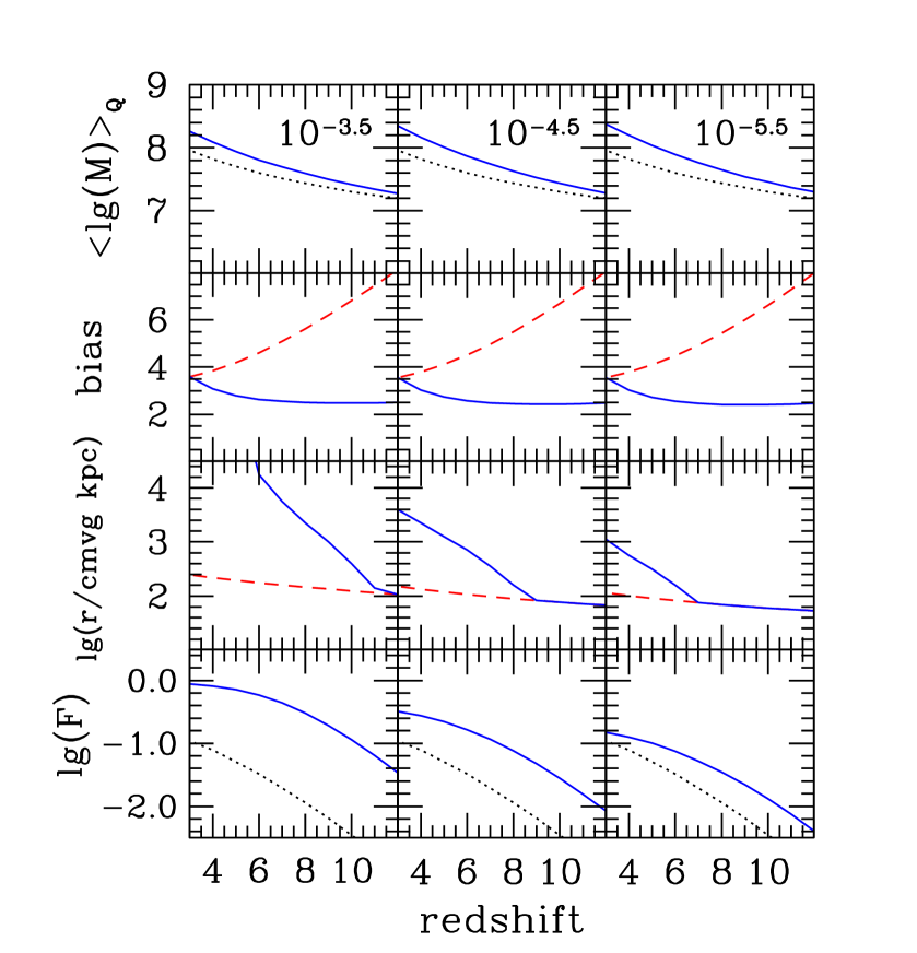
Figure 1: Properties of $T_{\rm vir}\geq 10^{4}$K enrichment for an energetic model with ${\cal E}_{\rm g}=10^{-3.5}$ (left column), the fiducial model with ${\cal E}_{\rm g}=10^{-4.5}$ (center), and a weak outflow model with ${\cal E}_{\rm g}=10^{-5.5}$ (right). Top row: Porosity-weighted average source mass as a function of redshift (solid) as compared to the minimum mass (dotted). Second row: Porosity-weighed average bias $\left<b\right>_{Q}$ (dashed), and bias normalized versus $z=3$, $\left<b\right>_{Q}\times D(z)/D(3)$ (solid) which tracks the evolution of the correlation function as in eq. (7). Third Row: Volume-weighed average comoving outflow size, $\left<r_{s}\right>_{Q}$ (dashed), and the typical comoving size of enriched region, $\max\left\{r_{\rm overlap},\left<r_{s}\right>_{Q}\right\}$ (solid), which can be significantly larger due to overlapping sources. Bottom Row: Simple $1-\exp(-Q)$ estimate of the filling factor (solid), and 1/2 of the collapse fraction (dotted), an estimate of the enriched gas falling back onto further generations of sources.

3 Results

3.1 Variations in Energy Input

The properties of three enrichment models with $T_{\rm vir}\geq 10^{4}$ K, and widely varying ${\cal E}_{\rm g}$ values are shown in Figure 1. In all cases, the average source mass closely follows the minimum allowed value. The reason for this behavior can be seen from a simple Sedov-Taylor estimate. In this case the physical radius goes as $R\propto(E/\rho)^{1/5},$ where $E$ is the energy of the blast and $\rho$ is the ambient density, and thus the comoving volume goes as

$$V_{b}\propto r_{b}^{3}\propto M^{3/5}(1+z)^{6/5}.$$ (6)

From eq. (4) the comoving number density goes as $1/M$ (with only a small correction from the $\frac{d{\rm ln}\sigma^{2}}{d{\rm ln}M}$ term) such that $Q\propto M^{-2/5}$. Notice that this is a general result, which follows from dimensional analysis. The smallest sources naturally dominate the enrichment process, an effect that is only amplified by complications such as the additional gravitational drag in large halos (Scannapieco et al. 2002) or the inefficiency of OB associations at driving winds from large galaxies (Ferrara et al. 2002). In fact only an extremely strong increase in efficiency with mass (${\cal E}_{\rm g}\propto M^{n}$, with $n\geq 2/3$) can alter this conclusion.

Similarly, the strong redshift scaling in eq. (6) means that for any given mass the earliest sources enrich most efficiently. This is due to the simple fact that a fixed comoving distance corresponds to a smaller physical distance at higher redshift, yet it has profound implications for the resulting spatial distribution. In the second row of Fig. 1, I plot the porosity-averaged bias for each of the ${\cal E}_{\rm g}$ models considered. The strong increase of $V_{b}$ at high-redshift means that the relatively rare, high-$\nu$ sources contribute most strongly to $Q$. This results in a high bias, as such rare sources are highly clustered relative to the lower-$\nu$ peaks that collapse at lower redshifts (e.g. Mo & White 1996). Again this is a general result, that arises from dimensional arguments, and the strong clustering seen in this figure can only be amplified by IGM transitions such as reionization, which remove lower-mass, lower-redshift (and hence lower-$\nu$) peaks (e.g. Klypin et al. 1999). Note that in general while bias increases with redshift, the amplitude of the correlation function is given by

$$\xi\left(r,z,\left<b\right>_{Q}\right)=\left[\left<b\right>_{Q}D(z)\right]^{2}\xi_{0}(r),$$ (7)

where $\xi_{0}(r)$ is the matter correlation function, linearly extrapolated to the present, and $D(z)$ decreases with redshift. Thus $\xi(r,z,\left<b\right>_{Q})$ remains roughly constant with redshift.

The strong clustering of enriched regions must be also taken into consideration when interpreting the typical sizes of enriched regions. In the third row of Figure 1, I plot $\left<r_{s}\right>_{Q}$, which again scales roughly as ${\cal E}_{\rm g}^{1/5},$ and is always smaller than 300 comoving kpc. In order to estimate the sizes of typical measured regions, however, we must also consider the overlapping of such bubbles. This can be estimated by considering the distance from the center of a typical source at which the product of the number density of neighboring sources $n(r_{\rm overlap})$ and the volume around each source is equal to one. In our formalism this gives

$$\left[1+\xi\left(r_{\rm overlap},z,\left<b_{L}\right>_{Q}\right)\right]\times Q=1,$$ (8)

where here it is more appropriate to calculate bias in the Lagrangian coordinate system that does not include the peculiar motions of the sources, as these motions were not included in our outflow model. This means $\left<b_{L}\right>_{Q}=\left<b\right>_{Q}-1$ (e.g. Mo & White 1996).

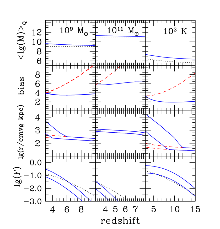
Figure 2: Properties of enrichment models as a function of minimum mass. Each row is labeled by the assumed $M_{\rm min}$ value, while the curves in each row are as in Figure 1. In the left column $M_{\rm min}=10^{9}{M_{\odot}},$ and I consider two cases with ${\cal E}_{\rm g}=10^{-4.5}$ and ${\cal E}_{\rm g}=10^{-3.5}$. In the center panel, $M_{\rm min}=10^{11}{M_{\odot}}$, and I take even higher energies of ${\cal E}_{\rm g}=10^{-3.5}$ and ${\cal E}_{\rm g}=10^{-2.5}$, which still give very low filling factors. Finally the right column shows the results of an extreme low-mass model in which $T_{\rm vir}\geq 10^{3}$K, and with low ${\cal E}_{\rm g}$ values of $10^{-4.5}$ and $10^{-5.5}$.

Despite the large range in ${\cal E}_{\rm g}$ values considered, the overlap radius is well above $\left<r_{s}\right>_{Q}$ at $z\leq 6$ for all three models. Thus the observed radii of enriched regions correspond to the sizes of typical overlapping groupings of sources, rather than the ejection radii from individual objects. Similarly, the growth of this scale with time is not caused by the expansion of material from a typical source, but rather is due to the formation of ever-larger groupings of overlapping bubbles. Indeed $r_{\rm overlap}$ increases drastically at late times in all three models, greatly outpacing the growth of the typical outflow as defined by $\left<r_{s}\right>_{Q}.$

The last row of Fig. 1 provides simple estimates of the filling factor of enriched regions. If the distribution of sources were completely uncorrelated, this could be computed directly from the porosity as $F=1-\exp(-Q),$ which corresponds to the solid lines in these panels. However, the strong overlapping between bubbles means that the true filling factor is probably somewhat smaller than this estimate. Finally, the dotted lines in these panels are 1/2 of the total collapse fraction, which is intended as a rough estimate of the gas that would fall back onto new sources in a more detailed simulation. This shows that infall is not important in these models, except for perhaps a small correction in the ${\cal E}_{\rm g}=10^{-5.5}$ case.

3.2 Variations in Minimum Mass

The second major parameter in our models is the minimum mass, which is raised to $10^{9}{M_{\odot}}$ in the cases shown in the left column of Figure 2, as might be caused by the increase in the IGM temperature following reionization, for example. This naturally raises $\left<\log(M)\right>_{Q}$ by over an order of magnitude, but the bias is much less affected, shifting from $\sim 3.5$ up to $\sim 4.0$. Thus although enrichment now occurs later, it is dominated by sources with similar $\nu$ values as in the $T_{\rm vir}\geq 10^{4}$ K case. Also as in the fiducial models, $r_{\rm overlap}>r_{s}$ in the observed redshift range, such that the scale of enriched regions is set by groupings of objects. Interestingly, as the filling factors are smaller in this case for the same values of ${\cal E}_{\rm g}$, raising the minimum mass actually lowers the sizes of typical enriched regions. However, there is probably a significant infall correction in this model.

These effects are intensified in the extreme $10^{11}{M_{\odot}}$ model shown in the center column of Figure 2. In this case, the bias rises to $\sim 5.5$, but the filling factors are so low that $r_{\rm overlap}<r_{s}$. The observed bubble radii are even smaller than in the $10^{9}{M_{\odot}}$ case, but now one is actually looking around individual sources. However, the very high energies and low filling factors make this case unlikely. Infall only makes this worse.

Finally, the right column of this figure shows the results of an extreme low-mass model in which the minimum virial temperature has been reduced to $10^{3}$ K. Even in this case $\left<b\right>_{Q}$ is about 3.5 at $z=3.$ The radii of enriched regions are again set by clustering, and are even larger than in the fiducial $T_{\rm vir}\geq 10^{4}$ K cases with the same choices of ${\cal E}_{\rm g}.$

4 Discussion

It is clear that the simplified models described above gloss over many of the detailed issues that are now beginning to be addressed numerically. Nevertheless, this simplicity serves to highlight how many counterintuitive observational trends can be understood from general arguments, which can be explored in more detail with future simulations.

Thus, the seeming contradiction between widespread outflows from large $z\sim 3$ galaxies and the lack of evolution in C iv number densities is most likely related to the $V\propto E^{3/5}$ scaling of outflows and the $1/M$ scaling in the number density of sources. Likewise the strong clustering of metal line systems is likely to be be reconciled with the efficient ejection of metals from small $M\lesssim 10^{10.5}{M_{\odot}}$ galaxies (Tremoni et al. 2004) because cosmological enrichment is dominated by early, rare sources, that can expand to cover the same comoving volume in shorter times. Finally, as strong clustering results in a significant overlap between sources, this may account for the large observed sizes of typical enriched regions, which require extremely large ejection energies to be explained by single sources (Kollmeier et al. 2003). Although there is much more to be learned, it is clear that the efficiency of lower mass, high-redshift sources and the overlap between bubbles should always be kept in mind when interpreting measurements of the spatial distribution of intergalactic metals.

- (1)
- (2) Adelberger, K. L., Steidel, C. C., Shapley, A. E., & Pettini, M. 2003, 584, 45
- (3) Aguirre, A., Schaye, J., Kim, T.-S., Theuns, T., Rauch, M., & Sargent, W. L. W. 2004, ApJ, 602, 38
- (4) Aguirre, A., Schaye, J., Hernquist, L. Kay, S., Springel, V., & Theuns, T. 2005, ApJ, 620, L13
- (5) Aracil, B., Petitjean, P., Pichon, C., & Bergeron, J. 2004, A&A, 419, 811
- (6) Benson, A. & Kamionkowski, M., & Hassani, S. H. 2005 MNRAS, submitted (astro-ph/0407136)
- (7) Bromm, V., Yoshida, N., & Hernquist, L. 2003, ApJ, 596, L135
- (8) Bruscoli, M. et al. 2003, MNRAS, 343, L41
- (9) Cen, R., Nagamine, K., & Ostriker. J. P. 2005, ApJ, submitted (astro-ph/0407143)
- (10) Ciardi, B., Ferrara, A., Governato, F., & Jenkins, A. 2000, Mon. Not. R. Astron. Soc., 314, 661
- (11) Dekel, A., & Woo, J. 2003, MNRAS, 344, 1131
- (12) Eisenstein, D. J. & Hu, W. 1999, ApJ, 511, 5
- (13) Ferrara, A., Pettini, M., & Shchekinov, Y. 2000, MNRAS, 319, 539
- (14) Haiman, Z., Rees, M., & Loeb, A. 1997, ApJ, 476, 458 (erratum 484, 985 [1997])
- (15) Kaiser, N. 1984, ApJ, 284, L9
- (16) Klypin, Anatoly, Kravtsov, A. V., Valenzuela, O., & Prada, F. 1999, ApJ, 522, 82
- (17) Kollmeier, J. A., Weinberg, D. H., Davé, R., & Katz, N. 2003, ApJ, 594, 75
- (18) Madau, P., Ferrara, A., & Rees, M. J. 2001, ApJ, 555, 9
- (19) Mo, H. J. & White, S. D. M. 1996, MNRAS, 282, 348
- (20) Qian, Y.Z. & Wasserburg, G. J. 2005, ApJ, in press (astro-ph/0501232)
- (21) Ostriker, J. P. & McKee, C. F. 1988, Rev. Mod. Phys., 60, 1
- (22) Pettini, M. 1999, in Chemical Evolution from Zero to High Redshift, Proc. ESO Workshop, ed. J. Walsh & M. Rosa (Berling: Springer), 233
- (23) Pettini, M. et al. , 2001, ApJ, 554, 981
- (24) Pettini, M., Madau, P., Bolte, M., Prochaska, J. X., Ellison, S., & Fan, X. 2003, ApJ, 594, 695
- (25) Pichon, C. et al. 2003, ApJ, 597, L97
- (26) Rauch, M., Sargent, W. L. W., Womble, D. S., & Barlow, T. A. 1996, ApJ, 467 L5
- (27) Rauch, M., Sargent, W. L. W., & Barlow, T. A. 2001, ApJ, 554, 823
- (28) Scannapieco, E., Ferrara, A., & Broadhurst, T. 2000, ApJ, 536, L11
- (29) Scannapieco, E., Ferrara, A., & Madau, P. 2002, ApJ, 574, 590
- (30) Scannapieco, E., Schneider, R., & Ferrara, A. 2003, ApJ, 589, 35
- (31) Schaye, J., Aguirre, A., Kim T.-S., Theuns, T., Rauch, M., & Sargent, W. L. W. 2003, ApJ, 596, 768
- (32) Schwartz, C. M., & Martin, C. L. 2004, ApJ, 610, 201
- (33) Sigward, F., Ferrara, A., & Scannapieco, E. 2005, MNRAS, in press (astro-ph/0411187)
- (34) Songaila, A. 1996 & Cowie L. L. 1996, AJ, 112, 335
- (35) Songaila, A. 2001, ApJ, 561, L153
- (36) Spergel, D. N. et al. 2003, ApJS, 14, 175
- (37) Springel, V. & Hernquist, L. 2003, MNRAS, 339, 289
- (38) Thacker, R., Scannapieco, E. & Davis, M. 2002, ApJ, 581, 836
- (39) Theuns, T., Viel, M., Kay, S., Schaye, J., Carswell, R. F.,& Tzanavaris, P. 2002, ApJ, 578, L5
- (40) Tremonti, C. A. et al. 2004, ApJ, 613, 898