Radiative equilibrium in Monte Carlo radiative transfer using frequency distribution adjustment

Abstract

The Monte Carlo method is a powerful tool for performing radiative equilibrium calculations, even in complex geometries. The main drawback of the standard Monte Carlo radiative equilibrium methods is that they require iteration, which makes them numerically very demanding. Bjorkman & Wood recently proposed a frequency distribution adjustment scheme, which allows radiative equilibrium Monte Carlo calculations to be performed without iteration, by choosing the frequency of each re-emitted photon such that it corrects for the incorrect spectrum of the previously re-emitted photons. Although the method appears to yield correct results, we argue that its theoretical basis is not completely transparent, and that it is not completely clear whether this technique is an exact rigorous method, or whether it is just a good and convenient approximation. We critically study the general problem of how an already sampled distribution can be adjusted to a new distribution by adding data points sampled from an adjustment distribution. We show that this adjustment is not always possible, and that it depends on the shape of the original and desired distributions, as well as on the relative number of data points that can be added. Applying this theorem to radiative equilibrium Monte Carlo calculations, we provide a firm theoretical basis for the frequency distribution adjustment method of Bjorkman & Wood, and we demonstrate that this method provides the correct frequency distribution through the additional requirement of radiative equilibrium. We discuss the advantages and limitations of this approach, and show that it can easily be combined with the presence of additional heating sources and the concept of photon weighting. However, the method may fail if small dust grains are included, or if the absorption rate is estimated from the mean intensity of the radiation field.

1 Introduction

The Monte Carlo method is a very powerful method to solve complicated radiative transfer problems. Apart from allowing virtually any geometrical distribution of sources and sinks, it has the potential to address a number of additional problems which form a serious challenge to the more conventional ray-tracing techniques. Possible problems that can be addressed include the calculation of polarization of scattered radiation (Code & Whitney 1995; Bianchi et al. 1996), the correct treatment of kinematical information in the radiative transfer problem (Mathews & Wood 2001; Baes & Dejonghe 2002; Baes et al. 2003), and inclusion of the clumpiness of the interstellar medium (Boissé 1990; Witt & Gordon 1996; Bianchi et al. 2000b).

In this paper we concentrate on another typical radiative transfer problem, the self-consistent heating and re-emission of an absorbing/scattering medium in thermal equilibrium with the radiation field. When dust grains absorb (mainly optical or UV) radiation from the ambient radiation field, they are heated, and they re-emit this absorbed energy at longer wavelengths, thereby altering the ambient radiation field. Hence the radiative transfer problem requires a simultaneous calculation of both the temperature distribution of the dust and the ambient radiation field.

As long as the geometry of the system is not too complicated, this problem can be solved with conventional techniques. In spherical geometry, the problem can be solved in a rather straightforward way using the traditional radiative transfer techniques (Rowan-Robinson 1980; Yorke 1980; Wolfire & Cassinelli 1986; Rogers & Martin 1986; Ivezić & Elitzur 1997). However, for more general two- and three-dimensional geometries the problem is much more difficult, and obtaining an exact solution becomes much harder with these conventional techniques (Efstathiou & Rowan-Robinson 1990, 1991; Sonnhalter et al. 1995; Men’shchikov & Henning 1997; Steinacker et al. 2003). This can be overcome with the Monte Carlo method, where there are no geometrical restrictions. The Monte Carlo method for radiative equilibrium radiative transfer calculations was pioneered more than two decades ago (Lefevre et al. 1982, 1983). Since then, various new techniques, optimizations and extensions have been proposed (Lucy 1999; Bjorkman & Wood 2001; Misselt et al. 2001; Ercolano et al. 2003b; Niccolini, Woitke & Lopez 2003) and the method has been applied to widely different environments, including stellar atmospheres (Lucy 1999; Wood et al. 2002), dusty galaxies (Bianchi et al. 2000a; Misselt et al. 2001), planetary nebulae (Ercolano et al. 2003a) and protostellar cores (Wolf et al. 1999; Stamatellos & Whitworth 2003).

One of these optimizations, proposed by Bjorkman & Wood (2001, hereafter BW), seems particularly interesting. These authors describe a technique in which iteration, which is an undesirable but necessary ingredient of the standard radiative equilibrium Monte Carlo techniques, can be avoided. However, it is not completely clear, in our opinion, whether the frequency distribution adjustment (hereafter FDA) technique, which the BW method employs, is an exact rigorous method, or whether it is just a good and convenient approximation. This narrow distinction is quite important, not only from an academic point of view. For example, Ercolano et al. (2003b) have developed an iterative Monte Carlo code for radiative equilibrium calculations in which the opacity of the obscuring medium depends on its temperature. They adopt the FDA technique in each iteration step. Any small deviations from the correct answer could culminate in larger errors after performing the same method at each iteration step.

It is therefore important to obtain a thorough theoretical understanding of the FDA method, and to investigate its advantages and limitations. This is the goal of the current paper. In section 2, we will describe the problem of radiative and thermal equilibrium Monte Carlo radiative transfer, and we focus on the FDA procedure proposed to avoid iteration. In section 3, we investigate the basis of the FDA procedure. We do this in a broader framework, and investigate the general problem of how a sampled distribution can be adjusted to a desired distribution by adding data points sampled from an adjustment distribution. We apply this to radiative equilibrium Monte Carlo radiative transfer in section 4, and compare the results with the method of BW. In section 5 we discuss the results and present the advantages and limitations of the FDA procedure.

2 Radiative equilibrium Monte Carlo radiative transfer

The basic idea of Monte Carlo radiative transfer is that a very large number of $L$-packets (often called photons or photon packets) are followed individually throughout the system while being emitted, scattered or absorbed. Each step in the lifetime of a single $L$-packet is governed by random events. First, we divide the total luminosity $L$ emitted by the radiation sources into a very large number $N$ of packets of equal luminosity $\delta L=L/N$. Next, the dust medium is divided into a number of dust cells, each of them representing a physical dust entity with a specific mass $M$ and temperature $T$ (the latter still has to be determined). We then start the actual Monte Carlo simulation by launching each of these $N$ packets randomly in the dusty medium. Each of them is assigned a random initial position ${\boldsymbol{r}}$ according to the geometry of the sources, a random initial propagation direction ${\boldsymbol{k}}$ and a random frequency $\nu$. During its journey through the dusty medium, the position and propagation direction of each $L$-packet changes, until it either leaves the system (and can be detected) or is absorbed by a dust grain.

2.1 Solution using iteration

In the standard application of the radiative equilibrium Monte Carlo calculations, we launch all direct source $L$-packets, follow them until they leave the system or are absorbed, and record the cell in which each absorption takes place. After launching and following all source $L$-packets, we calculate the dust temperature of each cell from the cell mass and the amount of absorbed luminosity. If $k$ packages have been absorbed in a dust cell, the temperature of this cell can be determined from the requirement that the total absorption rate ($\Gamma_{\text{abs}}$) in the cell must equal the total emission rate ($\Gamma_{\text{em}}$) from the cell. The former can be estimated by multiplying the number of $L$-packets that have been absorbed with the luminosity fraction $\delta L$ per $L$-packet, i.e.

$$\Gamma_{\text{abs}}=k\,\delta L=k\,\frac{L}{N},$$ (1)

whereas the latter is obtained from

$$\Gamma_{\text{em}}=4\pi\,M\int_{0}^{\infty}\kappa_{\nu}B_{\nu}(T)\,{\text{d}}\nu.$$ (2)

From the requirement that the absorption and emission rate balance each other,

$$\Gamma_{\text{em}}=\Gamma_{\text{abs}},$$ (3)

the new temperature $T$ of the cell can be determined. In order to conserve radiative equilibrium, we must launch a new set of $k$ $L$-packets, which should be distributed according to the emissivity of the dust cell,

$$j_{\nu}=\kappa_{\nu}B_{\nu}(T).$$ (4)

Hence each re-emitted $L$-packet must be assigned a frequency determined from the probability density function (hereafter PDF)

$$p(\nu){\text{d}}\nu=\frac{\kappa_{\nu}B_{\nu}(T)\,{\text{d}}\nu}{\int_{0}^{\infty}\kappa_{\nu}B_{\nu}(T)\,{\text{d}}\nu}.$$ (5)

By emitting these $k$ $L$-packets we assure that radiative equilibrium is satisfied in each cell.

Each of these re-emitted $L$-packets is again followed through the dust grid until either it is absorbed or it leaves the system. Again, we record the number of absorption events in each cell. This allows us to update the temperature of each cell, to determine the new emissivity, etc. This procedure naturally leads to an iteration, which stops when the temperature of each dust cell converges.

Unfortunately, Monte Carlo radiative transfer is a numerically demanding method, and so it would be very useful if somehow the iteration in this method could be either accelerated or avoided completely. Lucy (1999) has proposed a device to optimize the iteration. He argues that a much faster convergence can be achieved by applying a temperature correction and re-emission immediately after each individual absorption event. Thus, every single time an $L$-packet is absorbed, the temperature $T$ of the cell is updated to a new temperature $T+\Delta T$ and a new $L$-packet is re-emitted with the new emissivity of the cell $\kappa_{\nu}B_{\nu}(T+\Delta T)$. This $L$-packet is then followed until either it leaves the system or it is absorbed again. Hence the re-emitted $L$-packets enter the radiative transfer alongside the source $L$-packets, and also contribute to the heating of the dust. As a consequence, the temperature distribution and the radiation field of the system after the last $L$-packet leaves the system are closer to the equilibrium state, and fewer iterations are necessary to reach convergence.

2.2 Solution using the FDA method

Even with the improvements made by Lucy (1999), iteration remains necessary. Indeed, during the calculation, the temperature in each cell gradually increases, and the $L$-packets re-emitted in the beginning of the simulation are hence emitted from an incorrect frequency distribution (corresponding to a temperature which is too low). An extension of the idea of Lucy (1999) has been proposed by BW. Their aim is to correct, during each re-emission event, for the incorrect frequency distribution of the $L$-packets that have been re-emitted before. If this succeeds, then the system is in radiative and thermal equilibrium at all moments during the simulation, and after the last $L$-packet leaves the system, the correct temperature distribution and spectrum are obtained without any iteration at all.

Consider some stage in the Monte Carlo process, when $k$ $L$-packets have already been absorbed and re-emitted in a certain cell. The temperature of the cell has been gradually increasing from zero to $T$, and assume we somehow have managed to fine-tune the re-emission frequencies such that they all correspond to the emissivity $\kappa_{\nu}B_{\nu}(T)$. Now assume a $(k+1)$’th $L$-packet is absorbed, which increases the dust cell temperature to $T+\Delta T$, so that the emissivity changes to $\kappa_{\nu}B_{\nu}(T+\Delta T)$. To preserve radiative equilibrium, a new $L$-packet must be emitted with luminosity $\delta L$. Its frequency must be chosen in such a way that the ensemble of the $(k+1)$ re-emitted $L$-packets from this cell correspond to the new emissivity $\kappa_{\nu}B_{\nu}(T+\Delta T)$. BW argue that this can be satisfied if the $(k+1)$’th frequency corresponds to the difference emissivity

$$\Delta j_{\nu}=\kappa_{\nu}\Bigl{[}B_{\nu}(T+\Delta T)-B_{\nu}(T)\Bigr{]}.$$ (6)

Hence the $(k+1)$’th frequency should hence be drawn from the normalized PDF

$$\tilde{q}(\nu){\text{d}}\nu=\frac{\kappa_{\nu}[B_{\nu}(T+\Delta T)-B_{\nu}(T)]{\text{d}}\nu}{\int_{0}^{\infty}\kappa_{\nu}[B_{\nu}(T+\Delta T)-B_{\nu}(T)]{\text{d}}\nu}.$$ (7)

Note that this PDF is positive everywhere, because the Planck function is a monotonically increasing function of temperature. When the difference $\Delta T$ between the two temperatures is small, this expression can be approximated by

$$\tilde{q}(\nu){\text{d}}\nu\approx\frac{\kappa_{\nu}B^{\prime}_{\nu}(T)\,{\text{d}}\nu}{\int_{0}^{\infty}\kappa_{\nu}B^{\prime}_{\nu}(T)\,{\text{d}}\nu},$$ (8)

where $B^{\prime}_{\nu}(T)$ is the temperature derivative of the Planck function.

BW have implemented their technique and tested it on the set of benchmark models presented by Ivezić et al. (1997). They find good agreement with the benchmark results, and conclude that their FDA method works well. Furthermore, we have tested this method against the thermodynamic equilibrium test and shown that the method is indeed accurate: the temperature structure of a system embedded in an isotropic black-body radiation field was found to be uniform, with an accuracy which could be reduced to less than 0.1 K by simulating enough $L$-packets (Stamatellos & Whitworth 2003).

Two arguments, however, made us doubt whether this method is really an exact rigorous method, or whether it is just a very good and convenient approximation:

1. Equation (7) suggests that one can always adjust the spectrum of $k$ emitted frequencies from one PDF (corresponding to $T$) to another (corresponding to $T+\Delta T$) by simply adding one single frequency. Intuitively we expect that this is possible if the difference between these two temperatures is small, but that it will be very hard or impossible if the temperature difference is large. For example, when the temperature is very low, most of the radiation will be emitted at far-infrared or sub-millimeter wavelengths. When the temperature increase is sufficiently high, the new emissivity requires that most $L$-packets are emitted at optical or near-infrared wavelengths. Consequently, there is a limit on the temperature increase allowed by this method.

2. It seems logical that adjusting a sampled distribution by adding one more data point is much harder if many frequencies have been sampled before, than when only a small number of frequencies have been sampled. Therefore, one would in general expect that the ”adjustment PDF” $\tilde{q}(\nu){\text{d}}\nu$ would be an explicit function of the number $k$ of previously emitted $L$-packets.

In order to investigate this in detail, we study the issue of adjusting the behavior of a set of data points by adding new data points in a more general context in the next section, and apply the results to radiative equilibrium Monte Carlo radiative transfer afterwards.

3 Adjusting a previously sampled distribution

Assume $p(x){\text{d}}x$ and $r(x){\text{d}}x$ are two arbitrary PDFs, and consider the following question: is it possible to construct a third PDF $q(x){\text{d}}x$ which satisfies the condition that any set of $n+m$ data points, where the first $n$ data points are drawn randomly from $p(x){\text{d}}x$ and the last $m$ ones are drawn randomly from $q(x){\text{d}}x$, represents a set of data drawn randomly from $r(x){\text{d}}x$ ? In other words, can we find an ”adjustment PDF” that adjusts an arbitrary original PDF into an arbitrary altered PDF ?

The solution to this problem is based on the definition that the probability that any data point lies between $x$ and $x+{\text{d}}x$, when drawn randomly from a PDF $p(x){\text{d}}x$, equals $p(x){\text{d}}x$. Hence, when we draw $n$ random data points from this PDF, the expected number of them between $x$ and $x+{\text{d}}x$ is $n\,p(x){\text{d}}x$. Applying this to the total data set of $m+n$ data points, we can find the form of the required PDF. As we can simply add the number of data points in each interval, the expected number of data points between $x$ and $x+{\text{d}}x$ is given by

$${\text{d}}N(x)=n\,p(x){\text{d}}x+m\,q(x){\text{d}}x.$$ (9)

On the other hand, this sample of $m+n$ data points should represent a sample drawn randomly from the PDF $r(x){\text{d}}x$, and therefore we can also write

$${\text{d}}N(x)=(n+m)\,r(x){\text{d}}x.$$ (10)

From these two expressions, we find that the adjustment PDF should have the form

$$q(x){\text{d}}x=\left(1+\frac{n}{m}\right)r(x){\text{d}}x-\frac{n}{m}\,p(x){\text{d}}x.$$ (11)

However, it is not always guaranteed that this function is a valid PDF, because there is no a priori guarantee that it is positive over its entire domain. If this function does become negative, this means that it is impossible to adjust the PDF $p(x){\text{d}}x$ to $r(x){\text{d}}x$ by adding $m$ data points.

Whether or not it is possible to adjust one PDF into another depends both on the particular PDFs involved and on the ratio $k\equiv n/m$ of the number of data points already sampled to the number of data points which can be added. Logically, it will be easier to transform one PDF to another if the distributions are very similar, than when they are very different. Also, it will in general be easier to change one distribution into another one if many data points can be added to a few data points sampled before ($m\gg n$), than when only a few new data points can be added to a large set of already existing data points ($n\gg m$).

In appendix A, we demonstrate the adjustment of one PDF to another for gaussian distributions. If we want to adjust the original gaussian distribution into another gaussian distribution with the same dispersion but a different mean, we show that the resulting adjustment PDF will always be negative at some point, no matter how small the shift in the mean or the relative number of data points to be added. On the other hand, if we want to alter the original gaussian PDF to a gaussian PDF with the same mean but a larger dispersion, we find that this is possible in some cases. When the relative number of data points to add is too small or when the dispersion increase is too large, however, the adjustment is not possible.

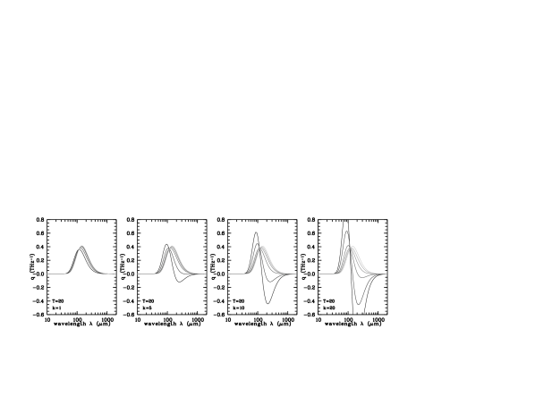
Figure 1: Examples of the adjustment PDF (14), corresponding to an opacity function $\kappa_{\nu}\propto\nu^{2}$ and $T=20$ K. The four different panels show the adjustment PDF for various values of $k$. In each panel, the different curves correspond to different values of the temperature increase, corresponding to $\Delta T=0.02$ K (light grey), 0.1 K, 0.2 K, 0.4 K, 1 K and 2 K (black). For small values of $k$ and $\Delta T$, the adjustment PDF is a positive function, and adjustment is possible. For large values of $k$ and/or $\Delta T$, the adjustment PDF is negative at long wavelengths, and adjustment is not possible.

4 Application to radiative equilibrium Monte Carlo radiative transfer

4.1 Determination of the adjustment PDF

With the general theorem from the previous section, we can return to the radiative equilibrium problem addressed in Section 2.2. What we need to do is to adjust a sample of $k$ frequencies drawn randomly from the PDF

$$p(\nu){\text{d}}\nu=\frac{\kappa_{\nu}B_{\nu}(T)\,{\text{d}}\nu}{\int_{0}^{\infty}\kappa_{\nu}B_{\nu}(T)\,{\text{d}}\nu}$$ (12)

to a sample of $k+1$ frequencies drawn from the PDF

$$r(\nu){\text{d}}\nu=\frac{\kappa_{\nu}B_{\nu}(T+\Delta T)\,{\text{d}}\nu}{\int_{0}^{\infty}\kappa_{\nu}B_{\nu}(T+\Delta T)\,{\text{d}}\nu},$$ (13)

by just adding one single frequency $L$-packet. Applying the general formula (11), we find that the last emitted $L$-packet should have a frequency drawn from the adjustment PDF

$$q(\nu){\text{d}}\nu=(1+k)\,\frac{\kappa_{\nu}B_{\nu}(T+\Delta T)\,{\text{d}}\nu}{\int_{0}^{\infty}\kappa_{\nu}B_{\nu}(T+\Delta T)\,{\text{d}}\nu}-k\,\frac{\kappa_{\nu}B_{\nu}(T)\,{\text{d}}\nu}{\int_{0}^{\infty}\kappa_{\nu}B_{\nu}(T)\,{\text{d}}\nu}.\qquad\quad$$ (14)

This formula can be easily interpreted in a physical way. When the $(k+1)$’th $L$-packet is absorbed, the temperature rises from $T$ to $T+\Delta T$. This last $L$-packet should then be re-emitted with a frequency sampled from the PDF corresponding to the new temperature, i.e.

$$P_{k+1}(\nu){\text{d}}\nu=\frac{\kappa_{\nu}B_{\nu}(T+\Delta T)\,{\text{d}}\nu}{\int_{0}^{\infty}\kappa_{\nu}B_{\nu}(T+\Delta T)\,{\text{d}}\nu}.$$ (15)

Additionally, we should account for the $L$-packets that were emitted previously with the incorrect frequency. Thus, we should re-emit the previous $k$ $L$-packets with a frequency sampled from the difference between the new and the old PDF,

$$P_{j}(\nu){\text{d}}\nu=\frac{\kappa_{\nu}B_{\nu}(T+\Delta T)\,{\text{d}}\nu}{\int_{0}^{\infty}\kappa_{\nu}B_{\nu}(T+\Delta T)\,{\text{d}}\nu}-\frac{\kappa_{\nu}B_{\nu}(T)\,{\text{d}}\nu}{\int_{0}^{\infty}\kappa_{\nu}B_{\nu}(T)\,{\text{d}}\nu}.\qquad(j=1\ldots k)$$ (16)

The above procedure is equivalent to emitting just one $L$-packet with the combined PDF as given by equation (14).

However, it is not guaranteed that this function corresponds to a valid PDF, because it can be negative. This is illustrated in figure 1, where we plot the adjustment PDF $q(\nu)$ for $T=20$ K and different values of the parameters $\Delta T$ and $k$. The opacity function adopted is a simple power law of frequency, $\kappa_{\nu}\propto\nu^{2}$. For small values of $k$, the adjustment PDF is positive for a large range of temperature shifts. However, when the number of previously generated frequencies $k$ is high, the adjustment PDF will be positive only for the smallest values of $\Delta T$. This behavior is also illustrated in figure 2, where we explicitly show the region in $(k,T,\Delta T)$ parameter space where adjustment is possible. The solid diagonal lines (different lines are shown for different values of $T$, but there is hardly any dependence on $T$) mark the border between positive and negative adjustment PDFs. For each number of data points $k$ and each temperature $T$, there is a maximum temperature increase $\Delta T_{\text{max}}(T,k)$ that can be allowed for adding one $(k+1)$’th frequency $L$-packet. As expected, this maximum temperature increase strongly decreases with increasing $k$.

4.2 Comparison with the BW adjustment PDF

The calculation in the previous subsection showed that the adjustment PDF (7) proposed by BW is in general not the same as the adjustment PDF (14). Moreover, we have shown that the latter does not represent a proper PDF for all of the parameters $(k,T,\Delta T)$. Indeed, for a given $k$ and $T$ there is a critical value of $\Delta T$, above which the adjustment PDF becomes negative. This observation suggests that the method by BW is an approximation rather than a rigorous solution, and even that the exact FDA procedure in Monte Carlo radiative transfer might not always be possible.

It is important to realize however, that not the entire $(k,T,\Delta T)$ parameter space will be covered during a simulation. Indeed, if a dust cell has a given temperature $T$ after absorbing and re-emitting $k$ $L$-packets, and the $(k+1)$’th $L$-packet is absorbed, the temperature rise $\Delta T$ is determined by the requirement of radiative equilibrium (3),

$$\int_{0}^{\infty}\kappa_{\nu}B_{\nu}(T+\Delta T)\,{\text{d}}\nu=\frac{(k+1)\,\delta L}{4\pi M}.$$ (17)

For the opacity function $\kappa_{\nu}\propto\nu^{2}$, the temperature increase $\Delta T$ can be calculated explicitly for each $T$ and $k$. Using the expression

$$\int_{0}^{\infty}\nu^{2}B_{\nu}(T)\,{\text{d}}\nu\propto T^{6},$$ (18)

one obtains after some algebra

$$\Delta T(T,k)=T\left[\left(1+\frac{1}{k}\right)^{1/6}-1\right].$$ (19)

This function is plotted as the dotted line in figure 2. This plot shows that $\Delta T(T,k)<\Delta T_{\text{max}}(T,k)$, i.e. at every step in the Monte Carlo simulation, the temperature increase is always small enough such that the adjustment PDF is positive. This proves that the FDA method in radiative equilibrium Monte Carlo radiative transfer works.

Knowing that the adjustment PDF (14) will always be positive for the expected temperature increase, we can compare the results with those of BW. From equation (17), we obtain that

$$\frac{\int_{0}^{\infty}\kappa_{\nu}B_{\nu}(T+\Delta T)\,{\text{d}}\nu}{\int_{0}^{\infty}\kappa_{\nu}B_{\nu}(T)\,{\text{d}}\nu}=\frac{k+1}{k}.$$ (20)

If we use this expression to eliminate $k$ from the adjustment PDF (14), we obtain

$$q(\nu){\text{d}}\nu=\frac{\kappa_{\nu}[B_{\nu}(T+\Delta T)-B_{\nu}(T)]{\text{d}}\nu}{\int_{0}^{\infty}\kappa_{\nu}[B_{\nu}(T+\Delta T)-B_{\nu}(T)]{\text{d}}\nu}\equiv\tilde{q}(\nu){\text{d}}\nu,$$ (21)

i.e. we recover the adjustment PDF proposed by BW.

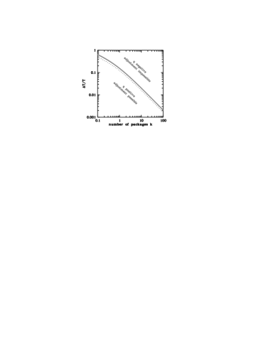
Figure 2: Region in $(k,T,\Delta T)$ parameter space in which the adjustment PDF (14) is positive. The opacity function is again $\kappa_{\nu}\propto\nu^{2}$. Different solid grey lines correspond to different values of the temperature $T$, but there is hardly any dependence on $T$. Each line shows for a given $T$ and $k$ the maximum temperature increase $\Delta T$ such that the adjustment PDF is positive. Hence, underneath the solid grey lines, adjustment is possible, above these lines, adjustment is impossible. The dotted line indicates the relative temperature increase expected from the radiative equilibrium requirement (see section 4.2).

5 Discussion

5.1 Efficiency of the method

The analysis in the previous section demonstrates that the FDA procedure proposed by BW provides the correct distribution of frequencies of the re-emitted $L$-packets. This demonstrates that the FDA algorithm is robust, and that at every step in the Monte Carlo simulation, the spectrum of the re-emitted $L$-packets is in agreement with the temperatures of the dust medium. As it avoids computationally costly iteration, the method is probably the most efficient way of doing thermal equilibrium radiative transfer calculation for arbitrary geometries.

One competitor might be the method pioneered by Niccolini et al. (2003), in which the determination of the temperature structure is separated from the Monte Carlo radiative transfer procedure. With the results of a single radiative transfer run with an initially guessed temperature distribution, they determine the correct temperature distribution and then scale the radiation field by the corresponding factors. Although their method also avoids performing several Monte Carlo simulation runs in an iterative loop, it still contains an iterative procedure to determine the temperature distribution. When the number of cells is small, this iteration is fairly quick, and this method is probably competitive with the FDA method of BW. When the number of cells is large, however, which may be necessary in realistic three-dimensional geometries without obvious symmetries, this iterative loop to determine the temperature distribution might be very difficult and time-consuming. This probably makes the FDA method the most efficient method for the general three-dimensional radiative equilibrium radiative transfer problem.

5.2 Extensions and optimizations

Although we have demonstrated that the method presented by BW represents the correct way to adjust the frequency distribution of the previously emitted $L$-packets, it should be kept in mind that the correct behavior is due to the additional requirement of local thermal and radiative equilibrium, as given in equation (17). Whenever deviations are made from this requirement, the extended technique might fail.

5.2.1 Photon weighting

We have assumed so far that all $L$-packets are luminosity packets with the same luminosity $\delta L$. When such an $L$-packet is absorbed, a new $L$-packet with a different frequency but with the same luminosity must be re-emitted. As such, the Monte Carlo simulation can be very inefficient in regions with low density. One option is to make the cells bigger such that more absorptions occur, but this decreases the spatial resolution. A more intelligent option is to drop the requirement that all $L$-packets must have the same luminosity, or equivalently, to introduce $L$-packet weights. By doing this, devices which reduce Poisson noise can be built into the Monte Carlo code, such as the principle of forced interaction or a peel-off technique (e.g. Cashwell & Everett 1959; Witt 1977; Yusef-Zadeh, Morris & White 1980; Niccolini et al. 2003).

We should consider whether such techniques are compatible with the FDA technique. To answer this question, assume that $k$ $L$-packets with luminosity $\delta L$ have been absorbed in a cell, that the temperature of the cell is $T$, and that a $k+1$’th $L$-packet is absorbed with a different luminosity, $w\,\delta L$. Clearly, an $L$-packet with this luminosity will have to be re-emitted, but what will be the shape of the adjustment PDF in this case ? In section 3 we saw that the adjustment PDF corresponding to adding $m$ data points to a set of $n$ existing data points only depends on the relative number $k=m/n$ of existing data points. Translating this to the current case means that the adjustment PDF corresponding to adding an $L$-packet with luminosity $w\,\delta L$ to a set of $k$ $L$-packets with luminosity $\delta L$, is equivalent to adding one $L$-packet with luminosity $\delta L$ to a set of $k/w$ $L$-packets with luminosity $\delta L$. The same formula (14) will be appropriate but with $k$ replaced by $k/w$. We should in general not consider $k$ as an integer number corresponding to the number of $L$-packets absorbed by the dust cell before the last absorption event, but rather as a real number corresponding to the ratio of the luminosity of the last absorbed $L$-packet to the total luminosity absorbed by the dust cell before the last absorption event. Because $k$ has naturally the same meaning in equation (1) for the absorption rate, the BW adjustment PDF will still be valid. $L$-packet weighting can therefore be combined easily with the FDA method.

5.2.2 Additional heating sources

The technique described in this paper considers the calculation of the temperature distribution of dust grains, which are in radiative equilibrium with the radiation field. In realistic astrophysical situations, heating by the ambient radiation field is often not the only source of dust heating. Dust grains can be heated by a variety of other astrophysical processes, such as viscous or compressional heating, collisions with hot electrons in an X-ray halo or collisions with cosmic rays. In this case, the condition of radiative equilibrium (3) is not satisfied, and should now be replaced by a more general equation

$$\Gamma_{\text{em}}=\Gamma_{\text{abs}}+\Gamma_{\text{add}},$$ (22)

where $\Gamma_{\text{add}}$ represents the amount of energy per unit time (the luminosity) gained by the dust cell due to other processes. If we assume that this factor in general depends on the position, size, etc. of the dust cell, but not on its temperature, it remains constant during the Monte Carlo simulation.

Although radiative equilibrium is not satisfied, it is straightforward to see that the FDA method is fully compatible with such additional heating sources. Indeed, it suffices, as in section 5.2.1, to consider $k$ as the ratio of the luminosity of the last absorbed $L$-packet to the total luminosity gained by the dust cell before the last absorption event. In particular, this means that the temperature $T_{0}$ of the dust cell at the beginning of the simulation is not zero, but is determined by

$$\int_{0}^{\infty}\kappa_{\nu}B_{\nu}(T_{0})\,{\text{d}}\nu=\frac{\Gamma_{\text{add}}}{4\pi\,M}.$$ (23)

The FDA method can therefore be combined easily with additional heating sources.

5.2.3 Very small dust grains

Another case where condition (17) is not satisfied occurs when the contribution of small dust grains is important. These dust grains undergo transient heating to temperatures well beyond the equilibrium temperature (Guhathakurta & Draine 1989). This means that the grains within a dust cell have a range of time-dependent temperatures characterized by a temperature probability function $P(T)$ rather than a single equilibrium temperature. Although more complex physics are involved here, their inclusion in Monte Carlo radiative transfer calculation is in principle similar to the normal radiative equilibrium radiative transfer (e.g. Misselt et al. 2001). So in principle, the FDA technique could also be applied to this more difficult problem. However, it can be expected that the relative temperature increase of small dust grains may be so large that negative adjustment PDFs are obtained. Therefore, in the case of transient heating by small dust grains, iteration can probably not be avoided.

5.2.4 An alternative estimate for the absorption rate

In this Monte Carlo method, we have estimated the absorption rate by multiplying the number of $L$-packets that have been absorbed with the luminosity fraction $\delta L$ per $L$-packet, as in equation (1). However, this way of estimating the absorption rate performs rather poorly in low density environments. A better way of estimating the absorption rate is to use its direct link to the mean intensity of the radiation field,

$$\Gamma_{\text{abs}}=4\pi\,M\int_{0}^{\infty}\kappa_{\nu}J_{\nu}{\text{d}}\nu.$$ (24)

As Lucy (1999) argues, the mean intensity in a given cell can be estimated through its relation to the energy density of the radiation field. We only have to add a path length counter in each cell and determine the total path length covered by all $L$-packets in the cell (see also Niccolini et al. 2003). The advantage of this method is that all $L$-packets entering the dust cell will contribute to the estimate of the absorption rate. Since generally only a small number of the $L$-packets entering a cell will be absorbed, it is clear that this method will give a better estimate of the absorption rate, and hence of the temperature of the dust cells.

If we estimate the absorption rate in this way however, the relation (17) will not generally be valid anymore, and there is no reason why the adjustment PDF (14) should be equal to the BW PDF (7). Therefore, for the FDA method to work correctly, it is necessary to estimate the absorption rate as in equation (1), which might be rather inefficient in environments with a low density. When performing radiative equilibrium Monte Carlo simulations, it is hence strongly recommended to construct the dust cells in such a way that the absorption probability is more or less equal in each of the cells.

6 Conclusions

We have evaluated critically the frequency distribution adjustment (FDA) method, a technique proposed by Bjorkman & Wood (2001) to optimize radiative equilibrium Monte Carlo radiative transfer simulations.

We first investigated the more general problem of trying to adjust the spectrum of a set of data points sampled from an arbitrary distribution by adding extra data points, such that the combined data set appears to be sampled from an arbitrary third distribution. We have determined the general shape this distribution must have, and shown that it is not always possible to adjust a set of data points in an arbitrary way. Whether this is possible, depends on the shape of the distributions and on the relative number of data points that have already been sampled.

We use this general theorem to investigate the theoretical basis of the FDA method. We demonstrate that the FDA method provides the correct frequency distribution for the re-emitted $L$-packet, because of the additional requirement of radiative equilibrium. We also show that the method can be easily extended with the use of weighted $L$-packets, and that additional heating mechanisms can be included in the simulation without violating the FDA method. However, the method may fail if small dust grains are included, or if the absorption rate is estimated in an alternative way.

Appendix A Example of adjusting a gaussian distribution

Suppose that we have sampled a set of $n$ data points from a gaussian PDF,

$$p(x){\text{d}}x=\frac{1}{\sqrt{2\pi}\sigma}\,\exp\left[-\frac{(x-\mu)^{2}}{2\sigma^{2}}\right]{\text{d}}x,$$ (A1)

and we want to add a number $m=n/k$ data points such that the total data set represents a sample taken from a different gaussian PDF.

First, assume the required PDF is a gaussian with the same dispersion, but we shift the mean over a distance $\Delta\mu>0$

$$r(x){\text{d}}x=\frac{1}{\sqrt{2\pi}\sigma}\,\exp\left[-\frac{(x-\mu-\Delta\mu)^{2}}{2\sigma^{2}}\right]{\text{d}}x.$$ (A2)

Using expression (11), we find the resulting adjustment PDF $q(x){\text{d}}x$. It is a straightforward exercise to see that this function will always be negative in the range

$$x<\mu+\frac{\sigma^{2}}{\Delta\mu}\ln\left(\frac{k}{1+k}\right)-\frac{\Delta\mu}{2}.$$ (A3)

So, no matter how small $k$ or $\Delta\mu$, the function $q(x){\text{d}}x$ will never represent a proper PDF, such that it is (in theory) impossible to shift the mean of a gaussian distribution by adding more data points.

Next, assume the required PDF is a gaussian with the same mean, but with a different dispersion $\sigma^{\prime}=(1+\delta)\sigma$,

$$r(x){\text{d}}x=\frac{1}{\sqrt{2\pi}(1+\delta)\sigma}\,\exp\left[-\frac{(x-\mu)^{2}}{2(1+\delta)^{2}\sigma^{2}}\right]{\text{d}}x.$$ (A4)

Again, the appropriate adjustment PDF $q(x){\text{d}}x$ can be obtained using equation (11). A similar exercise shows that this function becomes negative if,

$$(x-\mu)^{2}<\frac{2(1+\delta)^{2}\sigma^{2}}{(1+\delta)^{2}-1}\ln\left[\frac{(1+\delta)k}{1+k}\right].$$ (A5)

This condition will, however, never be satisfied if the right-hand side of this equation is negative, i.e. when $\delta<1/k$. In this case, the function $q(x)$ will therefore be positive for all values of $x$ and represents a valid PDF.

References

- (1) Baes M., Dejonghe H., 2002, MNRAS, 335, 441
- (2) Baes M., Davies J. I., Dejonghe H., Sabatini S., Roberts S., Evans R., Linder S. M., Smith R. M., de Blok W. J. G., 2003, MNRAS, 343, 1081
- (3) Bianchi S., Ferrara A., Giovanardi C., 1996, ApJ, 465, 127
- (4) Bianchi S., Davies J. I., Alton P. B., 2000a, A&A, 359, 65
- (5) Bianchi S., Ferrara A., Davies J. I., Alton P. B., 2000b, MNRAS, 311, 601
- (6) Bjorkman J. E., Wood K., 2001, ApJ, 554, 615 [BW]
- (7) Boissé P., 1990, A&A, 228, 483
- (8) Cashwell E. D., Everett C. J., 1959, A Practical Manual on the Monte Carlo Method for Random Walk Problems, Pergamom, New York
- (9) Code A. D., Whitney B. A., 1995, ApJ, 441, 400
- (10) Efstathiou A., Rowan-Robinson M., 1990, MNRAS, 245, 275
- (11) Efstathiou A., Rowan-Robinson M., 1991, MNRAS, 252, 528
- (12) Ercolano B., Barlow M. J., Storey P. J., Liu X.-W., 2003a, MNRAS, 340, 1136
- (13) Ercolano B., Morisset C., Barlow M. J., Storey P. J., Liu X.-W., 2003b, MNRAS, 340, 1153
- (14) Guhathakurta P., Draine B. T., 1989, ApJ, 345, 230
- (15) Ivezić Ž, Elitzur M., 1997, MNRAS, 287, 799
- (16) Ivezić Ž, Groenewegen M. A. T., Men’shchikov A., Szczerba R., 1997, MNRAS, 291, 121
- (17) Lefevre J., Bergeat J., Daniel J. Y., 1982, A&A, 114, 341
- (18) Lefevre J., Daniel J. Y., Bergeat J., 1983, A&A, 121, 51
- (19) Matthews L. D., Wood K., 2001, ApJ, 548, 150
- (20) Misselt K. A., Gordon K. D., Clayton G. C., Wolff W. J., 2001, ApJ, 551, 277
- (21) Lucy L. B., 1999, A&A, 344, 282
- (22) Men’shchikov A. B., Henning Th., 1997, A&A, 318, 879
- (23) Misselt K. A., Gordon K. D., Clayton G. C., Wolff M. J., 2001, ApJ, 551, 277
- (24) Niccolini G., Woitke P., Lopez B., 2003, A&A, 399, 703
- (25) Rogers C., Martin P. G., 1986, ApJ, 311, 800
- (26) Rowan-Robinson M., 1980, ApJS, 44, 403
- (27) Sonnhalter C., Preibisch T., Yorke H. W., 1995, A&A, 299, 545
- (28) Stamatellos D., Whitworth A. P., 2003, A&A, 407, 941
- (29) Steinacker J., Henning Th., Bacmann A., Semenov D., 2003, A&A, 401, 405
- (30) Witt A. N., 1977, ApJS, 35, 1
- (31) Witt A. N., Gordon K. D., 1996, ApJ, 463, 681
- (32) Wolf S., Henning Th., Stecklum B., 1999, A&A, 349, 839
- (33) Wolfire M. G., Cassinelli J. P., 1986, ApJ, 310, 207
- (34) Wood K., Wolff M. J., Bjorkman J. E., Whitney B., 2002, ApJ, 564, 887
- (35) Yorke H. W., 1980, A&A, 86, 286
- (36) Yusef-Zadeh F., Morris M., White R. L., 1984, ApJ, 278, 186