Gemini and Chandra observations of Abell 586, a relaxed strong-lensing cluster.

Abstract

We analyze the mass content of the massive strong-lensing cluster Abell 586 ($z=0.17$). We use optical data (imaging and spectroscopy) obtained with the Gemini Multi-Object Spectrograph (GMOS) mounted on the 8-m Gemini-North telescope, together with publicly available X-ray data taken with the Chandra space telescope. Employing different techniques – velocity distribution of galaxies, weak gravitational lensing, and X-ray spatially resolved spectroscopy – we derive mass and velocity dispersion estimates from each of them. All estimates agree well with each other, within a 68% confidence level, indicating a velocity dispersion of 1000 – 1250 km s^-1. The projected mass distributions obtained through weak-lensing and X-ray emission are strikingly similar, having nearly circular geometry. We suggest that Abell 586 is probably a truly relaxed cluster, whose last major merger occurred more than $\sim 4$ Gyr ago.

1 Introduction

In a Universe where structures are formed hierarchically, as the current $\Lambda$CDM paradigm predicts, larger objects are formed through merging and/or accretion of smaller systems and the most massive structures should be the youngest. In the present era of evolution of the universe, massive clusters of galaxies occupy the upper limit of the mass function of (nearly) virialized structures. This special characteristic makes clusters privileged objects for the study of structure formation and the nature of dark matter, which is believed to play a major role in this process (e.g. White & Rees, 1978; Kauffmann et al., 1999).

Cluster masses can be measured by several techniques, each one relying on different principles and simplifying assumptions, Consequently, their biases are also different. Two techniques – the kinematics of the member galaxies and the X-ray emission from the hot gas that fills the intra-cluster medium (ICM) – assume dynamical equilibrium. On the other hand, gravitational lensing, in its strong and weak regime, does not require such an assumption, depending directly of the cluster surface mass (see the reviews by, e.g., Fort & Mellier, 1994; Mellier, 1999).

The use of different techniques to measure mass distributions will likely give different mass estimates. This was first demonstrated by Miralda-Escudé & Babul (1995), who have found a systematic difference by a factor of $\sim 2$–3 between strong lensing and X-ray mass measurements, with the second method systematically producing smaller values. Allen (1998) claimed to have solved this problem after comparing results for clusters with and without cooling flows. He found that, for the former, X-ray and lensing mass estimates tend to agree, whereas for the latter the opposite happens. With the assumption that cooling flow clusters are dynamically more evolved, he concluded that this discrepancy is due to non-thermal processes (such as merger of sub-components) affecting the ICM in the central regions of non-cooling flow clusters.

Gravitational lensing is often claimed to be a more reliable method for cluster mass estimation, because it does not depend on equilibrium assumptions about the dynamical state of the cluster. Among dynamical mass estimators, the X-ray emission of the intra-cluster gas is preferred to galaxy dynamics, since the gas is a collisional component that reaches equilibrium faster than galaxies. In other words, gas is considered a better tracer of the gravitational potential than galaxies (see, e.g., Sarazin, 1988, Sect. 5.5).

On the other side, there are growing evidences that lensing masses for some clusters can be overestimated due to the presence of other massive components along the line of sight (Metzeler et al., 1999; Hoekstra, 2003). This seems to be the case for the strong lensing clusters A2744 (AC118) (Girardi & Mezzeti, 2001; Cypriano et al., 2004) and CL0024+16 (Czoske et al., 2002; Kneib et al., 2003). In these cases, distance information is needed (e.g., from redshift surveys) to disentangle clearly two or more components along the line of sight.

Therefore, the use of a multi-technique approach to investigate galaxy clusters (e.g., Smail et al., 1997; Valtchanov et al., 2002; Ferrari et al., 2003; Proust et al., 2003; Smith et al., 2003, 2004) is ideal for the study of these objects. Not only it does allow more reliable mass estimations, but it may also offer several hints on the physical state of such complex and evolving systems. The goal of this paper is to apply this approach to investigate the mass distribution and the dynamical state of the cluster Abell 586.

Abell 586 is a Bautz-Morgan type I cluster, at $z=0.17$, with Abell richness class 3. It presents copious X-ray emission ($L_{X}=1.11\times 10^{45}h_{50}^{-1}$ erg s^-1; Ebeling et al., 1998), with its peak coincident with the position of the brightest cluster galaxy (BCG). We have chosen this particular cluster for this study because of its high X-ray luminosity and the presence of strong lensing features, both implying a high mass content.

Dahle et al. (2002) reported a long faint blue arc at the northwest of the cluster central galaxy, and our optical observations with Gemini revealed a fainter arc at the opposite direction with respect to the BCG.

Recent X-ray studies of this cluster (Allen, 2000; White, 2000), using ROSAT images and ASCA spectra, have found ICM temperatures ranging from 6.1 to 8.7 keV, depending on the adopted model. A de-projection analysis made by Allen (2000) predicts a velocity dispersion of $1050^{+450}_{-250}$km s^-1 for this cluster. However, a weak-lensing mass measurement by Dahle et al. (2002) leads to a much larger velocity dispersion: $\sigma=1680^{+160}_{-170}$ km s^-1.

In this paper we present new optical and X-ray observations (Section 2) that allowed us to estimate the cluster mass based on galaxy dynamics, weak and strong lensing, and ICM temperature and surface brightness profiles (Section 3). In Section 4 we compare and discuss the results obtained with the different methods and, finally, we summarize our results and present our main conclusions in Section 5. We adopt hereafter $H_{0}=70~{}h_{70}$ km s^-1 Mpc^-1, $\Omega_{M}=0.3$ and $\Omega_{\Lambda}=0.7$. At the distance of Abell 586, one arcsecond corresponds to 2.9 kpc. All quoted uncertainties are for a confidence level of 1-$\sigma$, or 68%, unless stated otherwise.

2 Observations and data reduction

In this section we present the optical and X-ray data used in our analysis and describe the main steps in their reduction.

2.1 Gemini-North optical data

All optical observations discussed here were obtained using the Frederick C. Gillett Telescope (Gemini North) at Mauna Kea operating in queue mode. Imaging and multi-object spectroscopy were carried out with GMOS (Hook et al., 2002). Image and spectroscopic basic reductions (de-biasing, flat-fielding, wavelength calibration, etc.) were done in a standard way, with the GMOS package running under the IRAF environment.

2.1.1 Imaging

We observed the cluster Abell 586 on two occasions. The first time (period 2001B) as part of a survey for gravitational arcs in 8 clusters with X-ray luminosities larger than $10^{45}h_{50}^{-1}$erg s^-1 in the BCS catalog (Ebeling et al., 1998).

This imaging consisted of three single exposures with the g^′, r^′ and i^′ Sloan filters (Fukugita et al., 1996), the integration times being 300, 250 and 250 seconds, respectively. Atmospheric conditions were nearly photometric and the seeing, as measured by the FWHM of point sources, was $\sim$0.7″. With these observations we detected gravitational arcs in Abell 586, that had already been reported by Dahle et al. (2002).

During Gemini period 2002B, follow-up observations of the cluster were performed, comprising deeper r^′ imaging and also multi-object spectroscopy. The total exposure time for imaging was 20 minutes (4 $\times$ 300s). These new images were taken in photometric conditions, and the seeing of the combined image is again $\sim$0.7″.

In both cases we have used GMOS with $2\times 2$ binned pixels, leading to a pixel size of 0.145″. The observed field of view has 5.5′ on a side.

We use the program SExtractor (Bertin & Arnouts, 1996) to build galaxy catalogs, adopting, as detection criterion, that objects should have at least 10 contiguous pixels with values above the background plus 1.5 times its dispersion. For the first run, the galaxy catalogs start to become incomplete (i.e., the logarithmic number counts start to departure from a linear behavior) at 22.5, 22.5 and 22.0 mag, for g^′, r^′ and i^′ bands, respectively. The magnitude completeness limit for the second run data is r${}^{\prime}=24.5$ magnitudes.

2.1.2 Spectroscopy

The GMOS spectroscopic observations were done using a 400 line mm^-1 red optimized grating, with a central wavelength of 7000Å. This configuration resulted in spectra with a resolution of 7Å, or nearly five spectral pixels (as measured from the FWHM of calibration lamp lines), covering the range 5000–9200Å.

The observations were done with two masks, each one with roughly 30 slits, with single integration times of 34 minutes each. Slits in the central part of the mask were placed over the large gravitational arcs and other candidate lensed objects. The remaining slits were positioned over bright galaxies in the GMOS field.

Redshifts for galaxies with absorption lines were determined using the cross-correlation technique (Tonry & Davis, 1979) as implemented by the software RVSAO (Kurtz & Mink, 1998). We have used as templates the spectra of the NGC galaxies 1700, 1426, 3096, 4087, 4472, and 4751, observed with the 2.5-m Du Pont telescope of the Las Campanas Observatory, and a synthetic spectrum built from the stellar library of Jacoby, Hunter & Christian (1984).

All these templates were observed and reduced by Rodrigo Carrasco. More details can be found in Carrasco, Mendes de Oliveira & Infante (2005). Only object-template matches with the correlation coefficient parameter $R>3$ were considered successful. Typical formal errors in the radial velocities are smaller than 30 km s^-1.

For galaxies having prominent emission lines, the redshifts were also determined directly from these lines, but these measurements were adopted only when the velocity determinations by cross-correlation were doubtful ($R<5$). In all cases, the differences between the two determinations were both results are smaller than 150 km s^-1. In total, we obtained 44 reliable redshifts. The resulting redshifts for the cluster galaxies are summarized in Table 1, and for the other galaxies in Table 2.

Objects are identified using their J2000.0 coordinates, in the same fashion as Cohen & Kneib (2002), so that C088_3712 has coordinates R.A. = 07^h32^m08.^s8, DEC. = $+31\arcdeg 37\arcmin 12\arcsec$. The prefix “C” in the name means that the galaxy is a cluster member, otherwise the prefix is a “G”.

Table 1: Spectral data for Abell 586 galaxies.

(1)	(2)	(3)	(4)	(5)	(6)	(7)
Name	RA (2000)	DEC (2000)	z	R	r′ (AB Mag.)	Emission lines
C088_3712	07 32 08.81	31 37 12.5	0.1686	7.7	18.82	H$\beta$, [OIII], [OI], [NII], H$\alpha$, [SII]
C093_3835	07 32 09.33	31 38 35.1	0.1687	6.7	20.12	$\cdots$
C094_3542	07 32 09.39	31 35 42.1	0.1739	6.2	19.75	$\cdots$
C107_3616	07 32 10.68	31 37 24.8	0.1744	13.7	18.84	$\cdots$
C107_3725	07 32 10.74	31 36 16.5	0.1728	7.4	18.86	H$\beta$, [OIII], [OI], [NII], H$\alpha$, [SII]
C118_3731	07 32 11.79	31 37 31.2	0.1699	12.9	18.34	$\cdots$
C123_3605	07 32 12.35	31 36 04.7	0.1665	6.5	20.62	$\cdots$
C127_3828	07 32 12.74	31 38 27.8	0.1655	6.0	20.86	$\cdots$
C131_3619	07 32 13.13	31 36 18.6	0.1597	$\cdots$	20.14	H$\beta$, [OIII], [HeI], [OI], [NII], H$\alpha$, [SII]
C137_3845	07 32 13.70	31 38 44.5	0.1714	12.8	18.87	$\cdots$
C144_3717	07 32 14.42	31 37 17.3	0.1730	13.0	18.04	$\cdots$
C156_3838	07 32 15.56	31 38 37.7	0.1767	10.4	19.65	$\cdots$
C157_3723	07 32 15.65	31 37 22.7	0.1802	14.4	18.53	$\cdots$
C163_3727	07 32 16.32	31 37 27.2	0.1698	10.8	19.75	$\cdots$
C169_3839	07 32 16.86	31 38 39.3	0.1683	14.4	18.54	$\cdots$
C171_3650	07 32 17.07	31 36 50.0	0.1738	5.9	18.23	H$\beta$, [OIII], [OI], [NII], H$\alpha$, [SII]
C176_3744	07 32 17.56	31 37 43.8	0.1658	5.5	20.41	$\cdots$
C177_3857	07 32 17.69	31 38 57.3	0.1679	13.0	18.06	$\cdots$
C186_3846	07 32 18.64	31 38 46.5	0.1673	$\cdots$	20.96	H$\beta$, [OIII], [NII], H$\alpha$, [SII]
C187_3846	07 32 18.71	31 38 46.0	0.1595	4.9	20.96	$\cdots$
C197_3726	07 32 19.74	31 37 26.3	0.1754	7.2	21.70	$\cdots$
C223_3818	07 32 22.27	31 38 17.9	0.1720	16.3	19.02	$\cdots$
C231_3752	07 32 23.08	31 37 51.9	0.1700	13.1	18.59	$\cdots$
C233_3800	07 32 23.26	31 38 00.3	0.1780	6.2	20.68	$\cdots$
C257_3708	07 32 25.75	31 37 07.7	0.1758	8.8	19.61	$\cdots$
C266_3652	07 32 26.61	31 36 52.2	0.1666	4.4	21.38	$\cdots$
C268_3631	07 32 26.77	31 36 31.0	0.1714	14.0	20.03	$\cdots$
C273_3618	07 32 27.29	31 36 17.9	0.1715	8.0	19.58	$\cdots$
C276_3652	07 32 27.57	31 36 51.5	0.1725	21.3	18.52	$\cdots$
C281_3813	07 32 28.14	31 38 12.6	0.1686	8.8	17.67	$\cdots$
C291_3557	07 32 29.11	31 35 56.5	0.1710	$\cdots$	20.52	[OIII], H$\alpha$, [SII]

Table 2: Spectral data for non-cluster members in the field of Abell 586.

(1)	(2)	(3)	(4)	(5)	(6)	(7)
Name	RA (2000)	DEC (2000)	z	R	r′ (AB Mag.)	Emission lines
G137_3635	007 32 13.67	31 36 35.2	0.2203	14.1	19.64	$\cdots$
G147_3845	007 32 14.72	31 38 45.1	0.2123	7.5	18.78	[NII], H$\alpha$
G181_3850	007 32 18.07	31 38 49.9	0.3050	5.3	18.66	$\cdots$
G194_3816	007 32 19.40	31 38 15.8	0.6093	$\cdots$	18.86	[OII], H$\beta$, [OIII]
G199_3734	007 32 19.92	31 37 33.6	1.4302	$\cdots$	21.87	[OII]
G208_3842	007 32 20.76	31 38 41.7	0.8973	$\cdots$	21.89	[OII]
G243_3809	007 32 24.29	31 38 08.7	0.2453	3.6	22.25	$\cdots$
G257_3837	007 32 25.69	31 38 37.1	0.3050	7.4	18.54	$\cdots$
G283_3604	007 32 28.33	31 36 04.2	0.8563	$\cdots$	21.06	[OII]
G288_3703	007 32 28.78	31 37 03.3	0.1921	$\cdots$	20.56	[OIII], [NII], H$\alpha$
G298_3552	007 32 29.79	31 36 23.3	0.1912	4.3	19.21	[NII], H$\alpha$
G298_3623	007 32 29.80	31 35 51.6	0.2141	8.1	19.31	$\cdots$
G305_3734	007 32 30.52	31 37 34.1	0.0596	$\cdots$	19.16	H$\beta$, [OIII], [NII], H$\alpha$, [SII]

2.2 Chandra X-ray observation and data reduction

Abell 586 was observed in September 2000 by the Chandra satellite in a single 11.83 ksec exposure with ACIS-I camera (observation ID 530, P.I. Leon Van Speybroeck). The data were taken in Very Faint mode with a time resolution of 3.24 sec. The CCD temperature was $-120^{\circ}$C. The data was reduced using CIAO version 3.0.1 following the Standard Data Processing, producing new level 1 and 2 event files.

The level 2 event file was further filtered, keeping only ASCA grades 0, 2, 3, 4 and 6. We checked that no afterglow was present and applied the Good Time Intervals (GTI) supplied by the pipeline. No background flares were observed and the total livetime is 10.04 ksec.

We have used the CTI-corrected ACIS background event files (“blank-sky”), produced by the ACIS calibration team, available from the calibration data base (CALDB). The background events were filtered, keeping the same grades as the source events, and then were reprojected to match the sky coordinates of Abell 586 ACIS observation.

We restricted our analysis to the range [0.3–8.0 keV], because above 8.0 keV, the X-ray emission is largely background-dominated.

2.2.1 X-ray Imaging

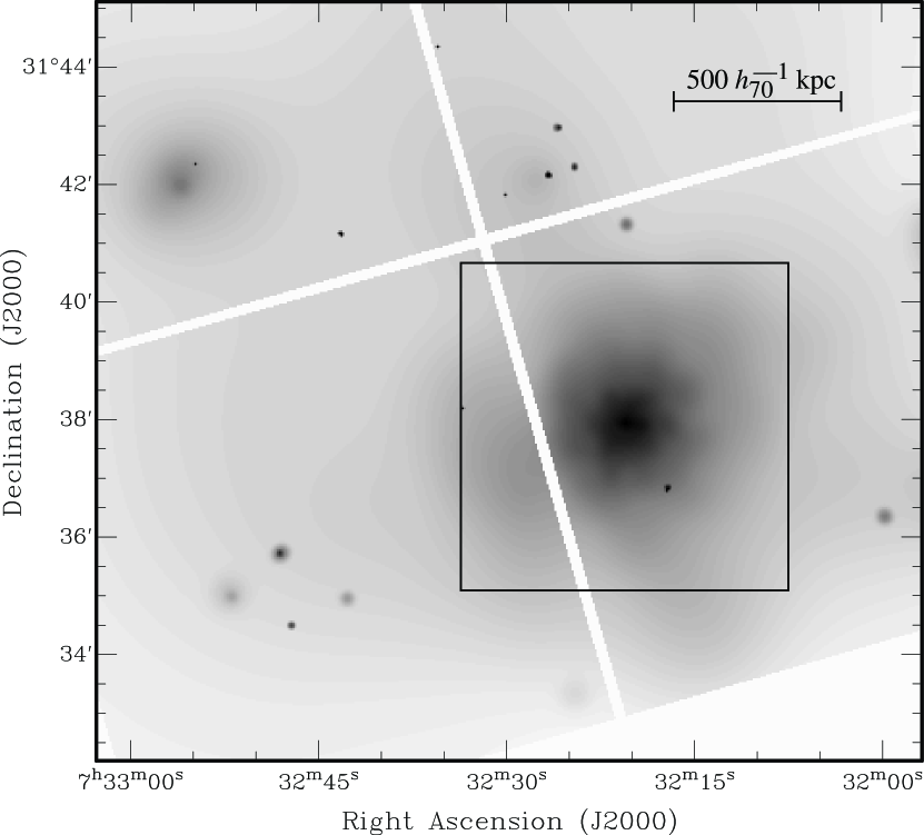
Figure 1: Chandra ACIS-I X-ray adaptively smoothed image of Abell 586 in the [0.3–8.0 keV] band, corrected by the exposure map and binned by a factor of 4. The center of the cluster is on the I3 chip (bottom right). There are also a number of point sources and a faint, extended source on the I0 chip (top left). The square ($5.5^{\prime}$ on a side) centered on the cluster shows the GMOS field of view.

We have constructed an adaptively smoothed image in the [0.3–8.0 keV] band using the csmooth tool from CIAO. The exposure map was generated by the script merge_all, where we have calculated the spectral weights, needed for the instrument map, using the cluster total spectrum, i.e., the spectrum obtained inside a circle concentric with the cluster, with a radius of 5 arcmin (about the GMOS field of view). We first smoothed the raw image, then the exposure map, using the scale map produced by the smoothing of the raw image, and finally divided the smoothed raw image by the smoothed exposure map. The result is shown in Figure 1.

The X-ray cluster emission can be detected up to 5 arcmin ($0.87h_{70}^{-1}$ Mpc) and is fairly symmetric. There is a strong point source at 78 arcsec from the center toward the Southwest that we identify with an active galaxy C171_3650 (cf. Table 1).

The absence of significant substructure in the X-ray map suggests that the last major merger with clusters with masses larger than 1/4 the Abell 586 mass occurred on a timescale longer than the cluster relaxation time. Roughly, the relaxation time is of the order of the dynamical time, $\tau_{d}\sim(G\overline{\rho})^{-1/2}$ where $\overline{\rho}\sim 340\Omega_{M}\rho_{c}$ inside the virial radius for a $\Lambda$CDM cosmology. Thus, $\tau_{d}\sim 4h_{70}^{-1}$Gyr and we suggest that the last major merger was at least 4 Gyr ago. Such a rough estimate usually agrees with $N$-body simulation results (e.g. Roettiger et al., 1998; Rowley et al., 2004).

2.2.2 X-ray Spectroscopy

For the spectral analysis, we have computed the weighted redistribution and ancillary files (RMF and ARF) using the tasks mkrmf and mkwarf from CIAO. These tasks take into account the extended nature of the X-ray emission. Background spectra were constructed from the blank-sky event files and were extracted at the same regions (in detector coordinates) as the source spectra that we want to fit.

The spectral fits were done using xspec v11.3, restricting to the range [0.3–8.0 keV]. The X-ray spectrum of each extraction region was modeled as being produced by a single temperature plasma and we employed the mekal (Kaastra & Mewe, 1993; Liedahl et al., 1995) model. The photoelectric absorption – mainly due to neutral hydrogen – was computed using the cross-sections given by Balucinska-Church & McCammon (1992), available in xspec.

The overall spectrum was extracted within a circular region of 1.4 arcmin (243 kpc) centered on the X-ray emission peak. It was re-binned with the grppha task, so that there are at least 30 counts per energy bin. This radius was chosen because almost all emission is in this region, we can avoid the CCDs gaps, and we have all the spectrum extracted in a single ACIS-I CCD. Figure 2 shows the overall spectrum fitted to an absorbed mekal plasma.

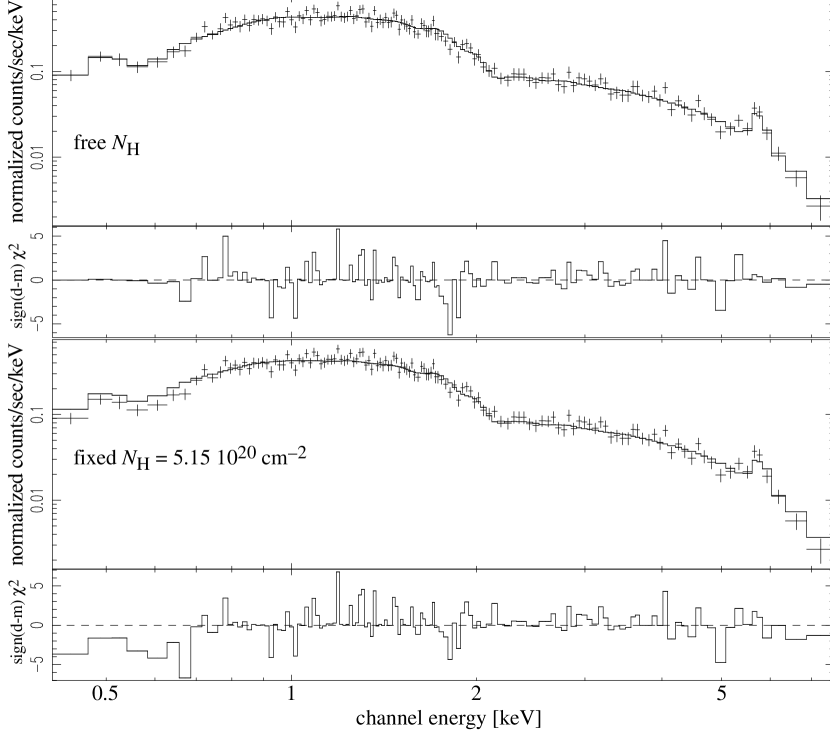
Figure 2: Chandra ACIS-I X-ray spectrum extracted in the central 1.4 arcmin ($245h_{70}^{-1}\,$kpc) superposed with a mekal plasma spectrum. Top: fit with $N_{\rm H}$ free. Bottom: fit with $N_{\rm H}$ fixed at the galactic value. Below each spectrum the residuals are shown expressed as the $\chi^{2}$ contribution of each binned energy channel.

A single-temperature gas fits well the overall spectrum; the reduced $\chi^{2}$ is $\chi^{2}/$d.o.f.$=132.7/133$. The temperature thus obtained is $kT=7.8_{-0.8}^{+1.0}$ keV (90% confidence level), in agreement with previous estimates; the metal abundance (hereafter, metallicity) is $Z=0.51_{-0.17}^{+0.18}~{}Z_{\odot}$ and the hydrogen column density is $N_{\rm H}=9.1_{-1.3}^{+1.4}\times 10^{20}$ cm^-2. The metallicity is higher than the average value of $1/3Z_{\odot}$ for clusters of galaxies.

The value of $N_{\rm H}$ obtained from the spectral fit is above the galactic value (Dickey & Lockman, 1990) which is $N_{\rm H}=5.15\times 10^{20}$ cm^-2 for the region of Abell 586. Not considering the uncertainties of the galactic $N_{\rm H}$ measurements, this excess is significant at a $3\sigma$ level. Such a level of significance may indicate that we are indeed detecting an X-ray absorption excess. The origin of such an absorption is controversial (Allen, 2000, and references therein), the most promising hypotheses being very cool molecular gas and/or dust grains that survives in the intracluster medium (ICM).

If we fix $N_{\rm H}$ at the galactic value, we obtain a much worst fit, $\chi^{2}/$d.o.f.$=157.6/134$ and a higher temperature, $kT=9.8_{-1.0}^{+1.3}$keV [this anti-correlation between the temperature and hydrogen column density is well-known, cf. Pislar et al. (1997)]. As can be seen in the residual plot of figure 2, this higher value of $\chi^{2}$ is mainly due to a poor fit at low energies ($E<0.7$keV). At high energies ($E>6.5$ keV), the fit is also a bit poorer than when $N_{\rm H}$ is considered as a free parameter.

2.2.3 Flux and luminosity

Table 3 summarizes the non-absorbed fluxes and luminosities obtained inside the central 1.4 arcmin field. We give the results in “soft” and “hard” bands, as well as the rest-frame bolometric luminosity (computed by extrapolating the plasma emissivity from 10 eV to 100 keV).

Table 3: Non-absorbed fluxes and luminosities in different energy bands. The energy band limits are given in keV.

flux	flux	flux	$L_{X}$	$L_{X}$	$L_{X}$
[0.5–2.0]	[2.0–10.0]	bolom.	[0.5–2.0]	[2.0–10.0]	bolom.
2.8	5.4	11.3	2.08	4.38	9.18

Note: flux units are $10^{-12}$erg cm${}^{-2}\,$s^-1.

Luminosity units are $10^{44}\,h^{-2}_{70}\,$erg s^-1.

Using the empirical relation $L_{X}$–$T_{X}$ obtained by Xue & Wu (2000), the bolometric X-ray luminosity (converted to $H_{0}=50\,$km s^-1 Mpc^-1) implies $kT=6.7\pm 0.7$, slightly cooler but in agreement (within the error bars) with the spectroscopically determined temperature.

3 Data analysis

3.1 Dynamics of galaxies

We obtained accurate redshifts for forty-four galaxies in the GMOS field of Abell 586, whose properties are summarized in Tables 1 and 2. Thirty-one of them, with redshifts between 0.16 and 0.18, constitute our spectroscopic sample of cluster galaxies. In Figure 3 we show examples of these spectra, and in Figure 4 their velocity distribution. The redshifts of the remaining galaxies have either $z<0.07$ or $z>0.19$.

Figure 3: Examples of spectra of cluster member galaxies. The upper and lower panels shows, respectively, the spectra of the galaxy with the best correlation coefficient (C276_3652) and the worst one (C266_3652). Both spectra have not been flux calibrated and have been smoothed using a boxcar filter with 6.8 Å (5 pixels) of length, for the sake of clarity.

Figure 4: Redshift distribution for the 31 galaxies in Table 1 with $0.16<z<0.18$. The bin size is 500 km s^-1. The tick-marks on the top of the panel represent individual galaxy velocities. The continuous line is a Gaussian function with bi-weighted location and scale values equal to $\langle z\rangle=0.1708$ and $\sigma=1161$ km s^-1, respectively.

We estimated the systemic redshift and the velocity dispersion of the cluster using the bi-weight estimators of the ROSTAT program (Beers, Flynn & Gebhartd, 1990). The resulting mean redshift is $\langle z\rangle=0.1708\pm 0.0006$ and the velocity dispersion is $\sigma=1161\pm 196$ km s^-1.

This value of $\langle z\rangle$ compares very well with the value obtained by Bottini (2001) using only 7 radial velocities of galaxies with very small projected distances to the BCG, $0.170\pm 0.001$. His determined velocity dispersion, $313\pm 70$ km s^-1, is much smaller than our value; this is not unexpected given his small sample.

There is a noticeable gap in the velocity histogram of $\sim 1500$ km s^-1 (in the cluster rest frame) between the two galaxies at $z\sim 0.160$ and the others. Excluding these two galaxies from our sample, the inferred values are $\langle z\rangle=0.1711\pm 0.0006$ and $\sigma=977\pm 130$ km s^-1. However, we consider that these galaxies should be kept in our sample because of the following reasons. Firstly, these galaxies are not excluded by a 3-sigma clipping selection. Secondly, the velocity histogram becomes too asymmetric after exclusion of the two galaxies (the ROSTAT asymmetry index increases from 0.48 to 0.96). Finally, because the difference between the BCG velocity and the systemic velocity which is normally small in cD clusters (Quintana & Lawrie, 1982), becomes larger, increasing from 121 to 221 km s^-1   in the cluster rest-frame.

We also verified the effect on the velocity dispersion caused by the 6 emission line galaxies, concluding that their removal from the calculation does not cause any appreciable change in $\sigma$.

Despite the internal robustness of the velocity dispersion found here, a word of caution is warranted. All galaxies used in this analysis lie within a radius of $570\,h_{70}^{-1}\,$kpc from the cluster center ($\sim 0.4R_{\rm vir}$; see Section 3.3). In order to understand more clearly the dynamics of this cluster, a larger set of velocities obtained over a larger field is required, as has been clearly demonstrated by, e.g., Czoske et al. (2002).

3.2 Weak Gravitational Lensing

3.2.1 Galaxy shape measurements

To estimate the cluster mass distribution through weak lensing, it is necessary to measure accurately the ellipticity of the background galaxies, which includes the effects of distortions introduced by the cluster gravitational potential.

The determination of galaxy shapes was performed using the method described in detail by Cypriano et al. (2004). Here we only summarize the main steps of this procedure.

The program im2shape (Bridle et al., 2002) is the basic tool we used for shape measurements. This program uses Bayesian methods to fit astronomical images as a sum of two-dimensional Gaussian functions with elliptical bases. Each of them is fully defined by six parameters: two Cartesian center coordinates, ellipticity, position angle, semi-major axis size and the amplitude. Moreover, im2shape deconvolves the fitted result by using a PSF, given also in terms of a sum of two-dimensional Gaussians, thus recovering an unbiased and accurate estimation of the object’s shape.

im2shape was first used to map the PSF over the whole GMOS field of view, by determining the shape of unsaturated stars, which have been selected based on their FWHM. For the stars, we prevented im2shape to do any deconvolution by using a Dirac’s delta function as the input PSF.

¿From the original sample of stars we kept only those that actually sample the local PSF. This has been done through a sigma-clipping process, where stars with too deviant ellipticities or position angles were removed. The remaining stars map a PSF which is nearly constant over the field, with average ellipticity of 0.056 (or 5.6%) and major axis oriented nearly East-West.

The next step is to run im2shape for galaxies. As galaxy images have more complex shapes than stars, they were modeled by a sum of two two-dimensional elliptical Gaussians with the same center, ellipticity and position angle. For each galaxy, the input PSF was calculated using their five closest stars.

3.2.2 Sample selection

Once we have measured the galaxy shapes, we need to identify the background galaxies, which can be used as probes of the cluster shear field. These galaxies constitute what we call the weak-lensing sample. Since their redshift is unknown, they were selected by their magnitudes and colors (when available). We have included in the weak-lensing sample only galaxies fainter than r${}^{\prime}=23.5$ and with (r^′ - i^′) colors not closer than 0.2 mag to the cluster red sequence. These criteria are adequate because the number density radial profile of the weak-lensing sample is nearly flat and does not decrease with increasing radius, as one would expect if there was significant contamination by cluster members.

In order to select a good quality weak-lensing sample, we kept only objects having errors on the tangentially projected ellipticities (with respect to the cluster center) smaller than 0.35. The resulting weak-lensing sample has 276 galaxies; the faintest has r${}^{\prime}=25.6$ mag., and the average magnitude in this sample is r${}^{\prime}=24.8$.

3.2.3 Mass distribution

The information on the shape of these galaxies (and the corresponding errors) was used to feed the software LensEnt (Bridle et al., 1998; Marshall et al., 2002) which, based on a maximum entropy method, reconstructed the projected mass density distribution of Abell 586. The resulting mass contours can be viewed in Figure 5. This map has been smoothed with a two-dimensional Gaussian with FWHM = 2.0′, that maximizes the likelihood of the reconstructed mass density given the data.

The mass distribution presented in this figure, showing a single mass clump associated with the BCG, is qualitatively very similar to the X-ray emission. This strongly suggests that the central region of Abell 586 is indeed in dynamical equilibrium. It is also worth noticing an extension towards the SE direction of the cluster, which is present both in the X-ray and weak-lensing contours. Our map is also in qualitative agreement with the weak-lensing mass map produced by Dahle et al. (2002), despite of a small offset in the peak position which, however, is within the resolution of both maps.

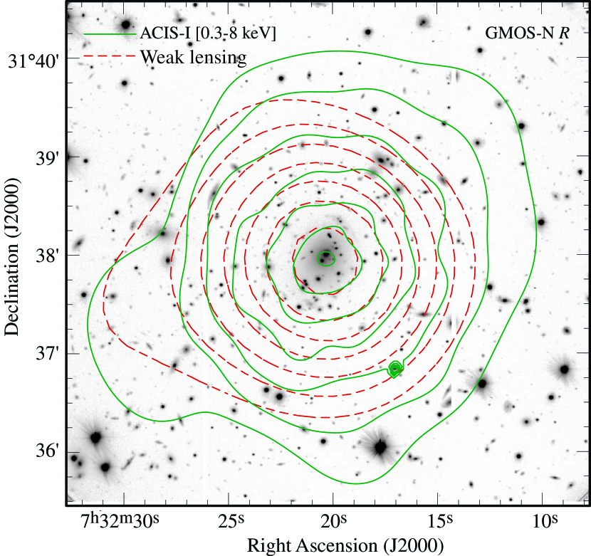
Figure 5: GMOS image of the central region of Abell 586 superimposed with logarithmically spaced X-ray isophotes (continuous lines) and weak lensing reconstructed mass density (dashed lines). The X-ray point source near the southwest corner is the Seyfert 1 galaxy C171_3650.

3.2.4 Radial shear profile

Very often the shear profile is fitted by a singular isothermal profile (SIS; e.g. Mellier, 1999). This model is very convenient because it has a single parameter, the Einstein radius, $\theta_{E}$, and allows direct comparisons with results already obtained for this and other clusters. Besides, it offers a rough approximation when only the central part of the cluster can be accessed, as in the present case. In this model, $\theta_{E}$ is directly related to the cluster velocity dispersion by the expression:

$$\theta_{E}=4\pi{\sigma^{2}\over c^{2}}\beta\,,$$ (1)

where $\beta$ is the ratio of $D_{ls}$, the angular diameter distance between the lens and the source, over $D_{s}$, the angular diameter distance to the source.

We adopt a simple parametric model for the mass distribution, the singular isothermal profile (SIS). More complex models are not appropriate, because our data has a rather high noise level due to the small number of galaxies to probe the shear field. Additionally, this kind of profile is widely used in studies of this type, allowing a simple comparison with other clusters.

To estimate the average $\beta$ of our sample we have used the catalog of photometric redshifts for the HDF of Fernández-Soto, Lanzetta & Yahil (1999). From this catalog, we selected a sample with the same bright limit and average magnitude as the present weak lensing sample. This catalog, however, does not have r^′ magnitudes; thus we have used I magnitudes, adopting the color (r${}^{\prime}-$ I) = 1.55. This color is typical for a Sbc galaxy at $z=0.8$ (Fukugita, Shimasaku & Ichikawa, 1995). This procedure resulted in an average value $\langle\beta\rangle=0.678$, corresponding to an average redshift of $0.78\pm 0.05$.

The best-fit shear profile (Figure 6) gives an Einstein radius of $30\pm 3$″, which translates into $\sigma=1243\pm 58$ km s^-1. The uncertainty of 58 km s^-1 is the statistical error of the fitting. It is important to mention that the determination of $\langle\beta\rangle$ is the major source of systematic uncertainties on the derived velocity dispersion and thus on absolute mass determinations through weak-lensing. For instance, if we adopt the color of a typical Sab or Scd galaxy, instead of a Sbc, the resulting velocity dispersion changes about $\pm 50$ km s^-1.

The value of the velocity dispersion we obtain here is significantly smaller than the one found by Dahle et al. (2002), $1680^{+160}_{-170}$ km s^-1. It is difficult to figure out the reasons of this discrepancy. One possible reason is that Dahle et al. have used the approximation $g\sim\gamma$ instead of $g=\gamma/(1-\kappa)$ used on the present work. Here, $g$ is the distortion, which is directly related to background-galaxy ellipticities, $\gamma$ is the gravitational shear, and $\kappa$ is the convergence or the projected mass density normalized with respect to a critical mass density:

$$\kappa\equiv{\Sigma\over\Sigma_{c}}=\Sigma\left({c^{2}\over 4\pi G}{1\over D_{l}~{}\beta}\right)^{-1}\,.$$ (2)

For strong lensing clusters like Abell 586, the assumption implicit in the approximation used by Dahle et al., i.e. $\kappa\sim 0$, is too strong, mainly for the cluster central regions. However, adopting this approximation in our sample, we get $\sigma=1353$ km s^-1. This valu is closer to the Dahle et al. result, but it is still significantly smaller. It is worth mentioning that the observations employed by them have similar depth to our observations. Dahle et al. observations were done with the 2.56-m NOT telescope with exposures of 5.4 ks in both $V$ and $I$ filters. After scaling and summing both exposures, the resulting imaging is about the same of the present 1.2 ks r^′ imaging with the 8.1-m Gemini-N telescope. Both detectors have also a similar field-of-view. In terms of image quality, however, our data is better. Dahle et al. reported a seeing FWHM of 1.0 and 0.8 arcsec for their $V$ and $I$ images, respectively, whereas for our data this value is 0.7 arcsec.

Figure 6: The shear profile for the cluster Abell 586. The filled symbols correspond to average ellipticities of the faint background galaxies projected tangentially to the cluster center. Each point represents the average of at least 55 galaxies of the weak-lensing sample. The open squares are the same, but for ellipticities projected in a direction 45° relative to the center. The solid line shows the best-fit SIS profile. The dashed line shows the Dahle et al. (2002) best SIS model ($\sigma$ = 1680 km s^-1).

3.2.5 Total mass

The mass profile can be directly measured from the shear data using the technique called aperture mass densitometry (AMD; Fahlman et al., 1994). This method is based on the single assumption that the surface mass density is circularly symmetric.

The AMD actually measures the difference between the mass density inside a given radius and the ring between this radius and a maximum radius of reference ($r_{max}$):

$$M_{AMD}(<r)=\pi~{}r^{2}\Sigma_{c}\,\zeta(r,r_{max})\,,$$ (3)

where $\zeta$ is defined by:

$$\zeta(r_{1},r_{max}) =\bar{\kappa}(r<r_{1})-\bar{\kappa}(r_{1}<r<r_{max})$$ (4)

$$={2\over 1-(r_{1}/r_{max})^{2}}\int^{r_{max}}_{r_{1}}{g_{t}(r)~{}d\ln{r}}\,,$$

where $g_{t}$ is the tangentially projected distortion, $r_{1}$ the radius in which the mass is measured, and $\bar{\kappa}$ the mean convergence.

We choose $r_{max}=150\,$arcsec (437 kpc at $z=0.17$), which is the largest radius fully contained within the field of view. Therefore, the total mass inside 422 kpc ($145\arcsec$) estimated by AMD is $(4.3\pm 0.7)\times 10^{14}\,M_{\odot}$. The mass profile can be seen, together with X-ray mass profiles, in Section 3.3.3.

¿From equation (3) it can be seen that the mass measured using the AMD method depends on $\Sigma_{c}$ and thus on $\beta$. Therefore the same systematical uncertainties related to the poorly known redshift distribution of the background sources, as previously discussed, applies here.

3.2.6 Strong-Lensing Features

The central region of Abell 586 (see Figure 7) shows several low surface brightness structures oriented tangentially to the cluster center, most of them with (g^′–i^′) colors up to 0.5 mag bluer than cluster ellipticals with similar brightness.

A prominent giant arc, already reported by Dahle et al. (2002), can be seen in the Northwest direction, distant 22 arcsec of the BCG center. There are several high surface brightness galaxies superimposed on this arc. At the opposite side of the central galaxy another giant arc, although fainter, can be appreciated in Figure 7 at 20 arcsec from the cluster center. Unfortunately, we could not determine the redshift of these arcs and, therefore, could not confirm whether they are multiple images of the same source.

We succeeded, however, to measure the redshifts of two arclets in the vicinity of the BCG, at 26.8 arcsec and 19.7 arcsec from the BCG center, whose orientations are nearly tangential to the direction of the cluster center. The spectra of these objects present emission and interstellar absorption lines, both typical of late-type galaxies. Their measured redshifts are 1.43 and 0.61, respectively (cf. Figure 7). No other objects with colors similar to those of these arclets were found, so no additional candidates for multiple images could be identified.

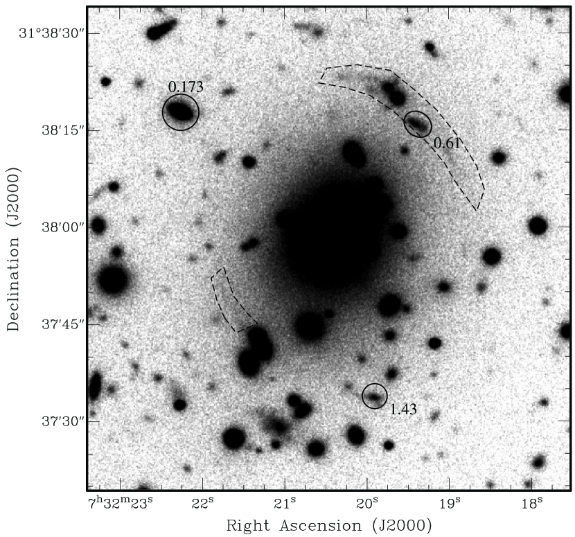
Figure 7: Optical image of central region of Abell 586. Objects with redshifts measured by us inside this field are marked. The dashed lines surround the gravitational arcs. This image shows a square region of 1.2′ on a side.

In the absence of multiple gravitational images it is not possible to model the cluster potential using the position of the arcs (like in Kneib et al., 1996). However, a rough estimate of the cluster mass inside the region enclosed by the arclets can be obtained assuming that they put a limit on the position of the Einstein radius. Under this assumption, we obtain, from the higher and lower redshift arclets, $\sigma$ equal to 1056 km s^-1 and 998 km s^-1, respectively.

This cluster shows another strong-lensing-like feature that deserves be mentioned. In Figure 8 we present a close-up of the spiral galaxy and cluster member C281_3813, that is at 1.7′ from the cluster center. What is remarkable in this figure is the presence of an arc-like object (indicated by an arrow). If this object has indeed a gravitational origin, it would be an uncommon example of strong-lensing by a late-type galaxy.

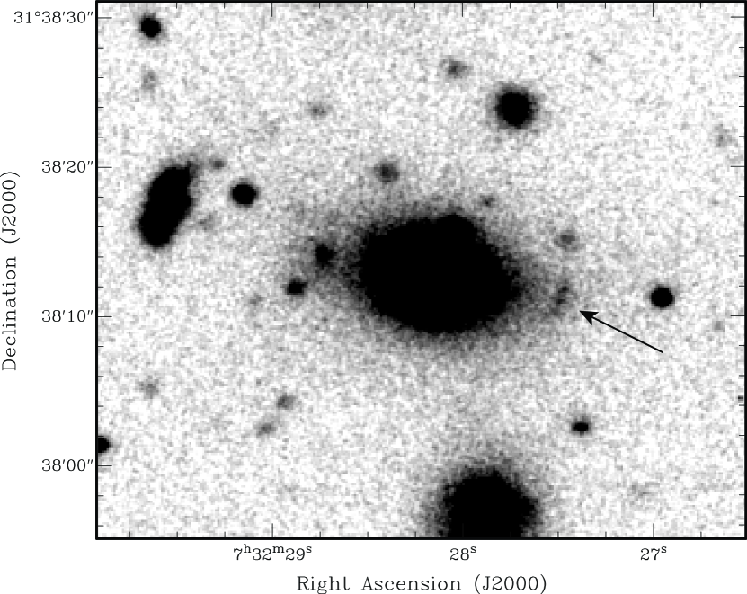
Figure 8: Image of the galaxy C281_3813, showing an arc-like object.

3.3 X-ray

3.3.1 X-ray brightness profile

The X-ray brightness profile of Abell 586 was obtained with the STSDAS/IRAF task ellipse. We have used the exposure map corrected image in the [0.3–8.0 keV] band, binned by a factor 4 (one X-ray image pixel has 2 arcsec). We have masked the CCDs gaps and source points. The brightness profile, shown in Figure 9, could be measured up to 500 arcsec ($1.46\,h_{70}^{-1}$Mpc) from the cluster center.

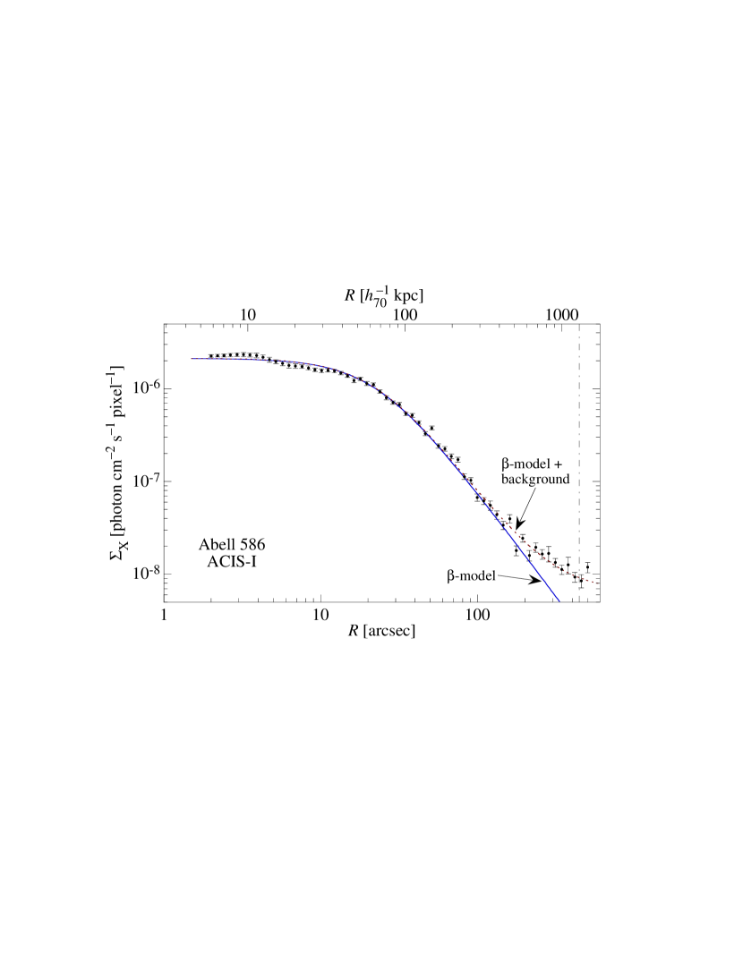
Figure 9: X-ray brightness profile. The full line shows the best fit $\beta$-model with $\beta=0.518\pm 0.006$ and $R_{c}=23.1\pm 0.6$ arcsec ($67\pm 2\,h_{70}^{-1}$kpc); the dotted line shows the $\beta$-model plus a constant background brightness (which was actually fitted). The vertical dotted-dashed line indicates the virial radius (cf. Section 11).

Using the $\beta$-model (Cavaliere & Fusco-Femiano, 1976) to describe the surface brightness radial profile,

$$\Sigma_{X}(R)=\Sigma_{0}\left[1+\left(\frac{R}{R_{c}}\right)^{2}\right]^{-3\beta/2}\,,$$ (5)

a least-squares fitting gives $\beta=0.518\pm 0.006$ and $R_{c}=23.1\pm 0.6$ arcsec ($67\pm 2\,h_{70}^{-1}$kpc). If we assume that the gas is approximately isothermal and distributed with spherical symmetry, there is a simple relation between the brightness profile and the gas number density, $n(r)$, i.e.,

$$n(r)=n_{0}\left[1+\left(\frac{r}{r_{c}}\right)^{2}\right]^{-3\beta+1/2}\,,$$ (6)

where $R_{c}=r_{c}$ (capital indicates projected 2D coordinates, lower case indicates 3D coordinates).

In order to estimate the central electronic density, $n_{0}$, we integrate the bremsstrahlung emissivity along the line-of-sight, in the central region, and compare with the flux obtained by spectral fitting of the same region. We obtain thus $n_{0}=(18.4\pm 1.5)\times 10^{-3}\,$cm^-3.

3.3.2 Temperature profile

We have computed the radial temperature profile using concentric circular annuli. For each annulus, defined by approximately the same number of counts (2000 counts, background corrected), a spectrum was extracted and fitted following the method described above, except that the hydrogen column density and metallicity were kept fixed at the mean best-fit value found inside 1.4 arcmin (i.e., $N_{\rm H}=9.1_{-1.3}^{+1.4}\times 10^{20}$cm^-2 and the metallicity $Z=0.5~{}Z_{\odot}$). Figure 10 shows the temperature profile.

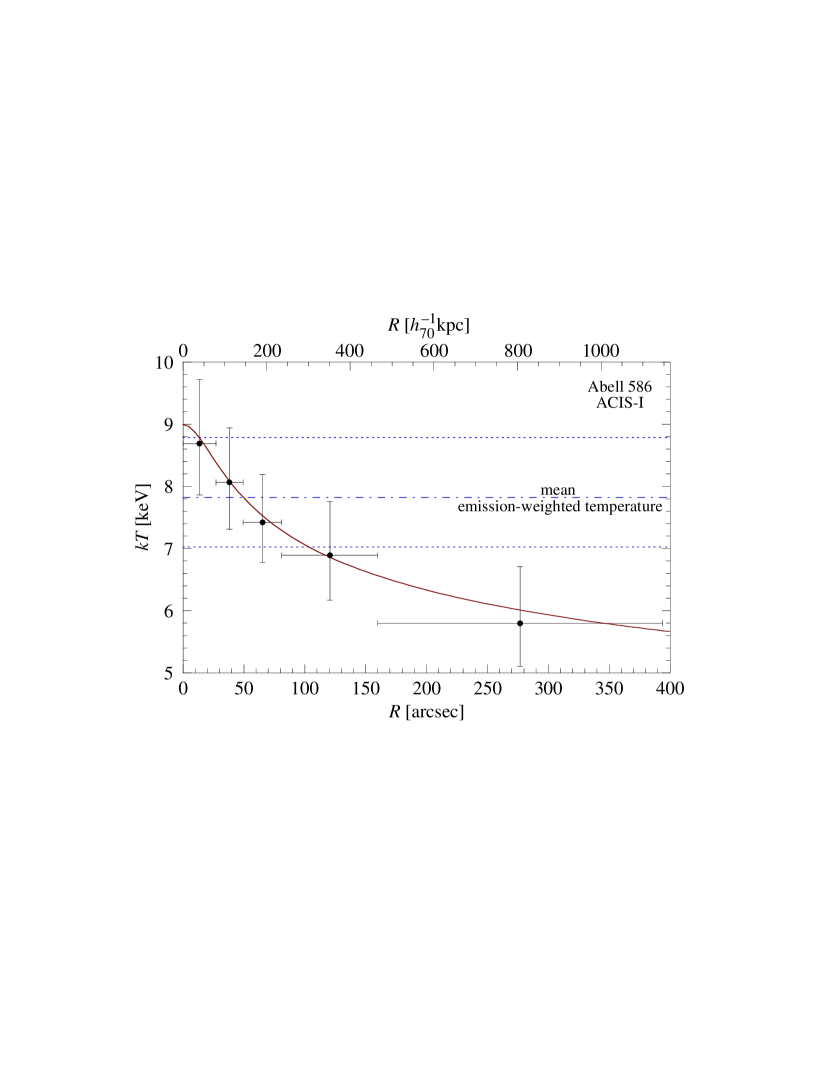
Figure 10: Temperature profile. The error bars are $1\sigma$ confidence level. The horizontal dotted-dashed line is the mean temperature inside 1.4 arcmin, $kT=7.8^{+1.0}_{-0.8}$ keV, the horizontal dotted lines correspond to 90% confidence level of the mean temperature. The full line shows the best-fit of the polytropic model (see text).

Since the temperature profile shows a clear gradient, we have tried a simple parametric form of the ICM temperature using a polytropic equation of state. It is not clear whether a polytropic model describes well the ICM. Indeed, Irwin et al. (1999) and De Grandi & Molendi (2002) argue that this is not a good description of the gas temperature profile in clusters. However, hydrodynamic simulations (Suto et al., 1998), theoretical models (e.g., Komatsu & Seljak, 2001; Dos Santos & Doré, 2002) and some observations (e.g., Markevitch et al., 1999; Finoguenov et al., 2001a) suggest that the gas may be described by a polytropic model, with polytropic index $\gamma$ roughly in the range $1.1\lesssim\gamma\lesssim 1.2$.

Therefore, we have fitted a polytropic temperature profile:

$$T(r)=T_{0}\left[1+\left(\frac{r}{r_{c}}\right)^{2}\right]^{-3\beta(\gamma-1)/2}\,,$$ (7)

where $r_{c}$ and $\beta$ are the values obtained with the $\beta$-model fitting of the brightness surface profile, and $T_{0}$ is the central temperature.

A standard least-square fit of Eq. (7) with only two free parameters, $T_{0}$ and $\gamma$, yields a rather good fit: $T_{0}=8.99\pm 0.34$ keV and $\gamma=1.10\pm 0.03$, cf. Figure 10. This value agrees with those found by Finoguenov et al. (2001b) and, being well below 5/3 (the ideal gas value), suggests that the gas may be in adiabatic equilibrium (see, eg., Sarazin, 1988, Sect. 5.2).

We note that this cluster does not present any sign of cooling in the very central part, at $R\approx 70\,h_{70}^{-1}\,$kpc, the smallest radius where we can extract a meaningful spectrum and measure the temperature. Either we lack the resolution to detect an eventual drop in temperature or the intracluster gas is not cooling. Since the central cooling-time is roughly

$$t_{\rm cool}\approx 5.8\times 10^{9}\frac{T_{\rm keV}^{1/2}}{n_{3}}\approx 10^{9}\,\mbox{years}\,,$$ (8)

then, if the gas is indeed not cooling, something must be heating it (as it was already realized for some clusters, e.g., Peterson et al., 2001). Heating by cluster merging seems improbable, given the apparent spherical symmetry of the X-ray emission. Other possibilities, like heating by AGN, thermal conduction, etc., may be playing a role in the energy budget of this cluster (e.g., Markevitch et al., 2003).

However, we may be simply not detecting an eventual drop in temperature because we lack the resolution. Using a sample of 20 clusters, Kaastra et al. (2004) show that the radius ($r_{c}$ in their paper) where the temperature drops in cooling-flow clusters is, with 2 exceptions, smaller than $70h_{70}^{-1}\,$kpc.

3.3.3 Gas and total masses

We estimate the gas mass simply by integrating the density given by Eq. (6), assuming spherical symmetry which, in this case, seems a good approximation (cf. Figure 5). The integrated gas mass is shown in the top panel of Figure 11.

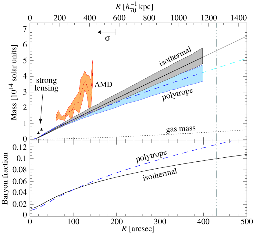
Figure 11: Top: X-ray dynamical mass profile assuming isothermal profile (full line), polytropic profile (dashed), weak-lensing mass profile using the AMD method (small dashed) and strong-lensing mass estimates (triangles). The shaded areas represents 1-$\sigma$ uncertainties. The arrow on the top of the panel marks the radius that contains all the galaxies used for the dynamical analysis. Bottom: Baryon fraction for isothermal (full line) and polytropic (dashed) temperature profiles. The vertical line indicates the virial radius.

Having the temperature profile, we also compute the “X-ray” dynamical mass (i.e., the dynamical mass determined from an X-ray observation, not to be confused with the mass of the X-ray emitting gas). Supposing hydrostatic equilibrium and polytropic temperature profile, the dynamical mass is given by:

$$M(r)=\frac{3kT_{0}\beta\gamma r_{c}}{G\mu m_{\rm p}}\left(\frac{r}{r_{c}}\right)^{3}\left(1+\left[\frac{r}{r_{c}}\right]^{2}\right)^{-1-\frac{3}{2}(\gamma-1)\beta}\,.$$ (9)

If $\gamma=1$, we have the usual isothermal mass profile. Here, $\mu\,m_{p}$ is the mean mass per particle ($\mu=0.6$ for a fully ionized gas with primordial He abundance) and $m_{\rm p}$ is the proton mass. The top panel of Figure 11 shows the dynamical mass profile estimated both with an isothermal ($\gamma=1$) and polytropic temperature profile ($\gamma=1.1$).

The gas mass at $R=400^{\prime\prime}$ ($1.16\,h_{70}^{-1}$Mpc) is $0.43\times 10^{14}M_{\odot}$. Depending on the assumed temperature profile, $M_{\rm dyn}=5.3\times 10^{14}M_{\odot}$ (isothermal case) and $M_{\rm dyn}=4.25\times 10^{14}M_{\odot}$ (polytropic case) within the same radius.

Virial radius and baryon fraction

We can now compute the radius corresponding to the density ratio $\delta=\bar{\rho}(r_{\delta})/\rho_{\rm c}(z)$. For $\delta=200$, we have the usual $r_{200}$; for the SCDM and $\Lambda$CMD cosmological models, $\delta=180$ and 340 correspond, respectively, to the virial radius (cf. Lacey & Cole, 1993; Bryan & Norman, 1998).

Taking into account the polytropic temperature profile, we use the formula in the appendix of Lima Neto et al. (2003) to compute the various $r_{\delta}$. Table 4 shows the results, where each column corresponds to a density ratio and the lines with “poly” and “isoth” refer to the polytropic and isothermal temperature profiles, respectively. Then, assuming a polytropic profile and the $\Lambda$CDM scenario, the virial radius is $r_{\rm vir}=1.26h_{70}^{-1}\,$Mpc, which corresponds to $R=430^{\prime\prime}$.

Table 4: Radius at different density contrast.

$\qquad\delta$:	180	200	340	500	2500	Model
$r_{\delta}$:	1.69	1.61	1.26	1.05	0.49	poly
arcsec	1.97	1.83	1.40	1.16	0.51	isoth

Obs.: $r_{\delta}$ is in units of $h_{70}^{-1}$Mpc.

Using the dynamical and gas mass profiles, we can derive the baryon fraction profile, $f(r)\equiv M_{\rm baryon}/M_{\rm total}$, assuming that the bulk of the baryons are in the ICM (i.e., $M_{\rm baryon}\approx M_{\rm gas}$). The galactic contribution to the baryon mass is taken into account following White et al. (1993) and Allen et al. (2002):

$$M_{\rm baryon}=M_{\rm gas}(1+0.16\,h_{70}^{0.5})\,,$$ (10)

where $M_{\rm gas}$ is the intracluster gas mass.

At $R=400$ arcsec, the baryon fraction is still rising. Its value at this point depends on the assumed temperature profile: for the isothermal and polytropic cases we have $f=0.10$ and 0.12, respectively. The baryon fraction determined here agrees with the usual values found in rich clusters (e.g. White & Fabian, 1995; Allen et al., 2002).

At the virial radius, defined above, we have $M_{\rm gas}=0.48\times 10^{14}M_{\odot}$, $M_{\rm dyn}=4.53\times 10^{14}M_{\odot}$, and $f=0.12$ (assuming a polytropic temperature profile).

4 Discussion

The mass determinations resulting from the application of four distinct techniques, based on different types of data, to the cluster Abell 586 are compared in this section discussed within the context of eventual deviations from a relaxed state.

In Table 5 are listed the velocity dispersions either measured or deduced in this paper through strong-lensing, X-ray, redshift survey, and weak-lensing methods, together with results of other authors.

Except for the velocity dispersion determined by Bottini (2001) and Dahle et al. (2002), all estimations agree well within at least a 68% confidence level. This result is strengthened when we compare the mass profiles provided by each technique (see Figure 11), although systematic differences within 2$\sigma$ between the (model dependent) measurements are noticed.

Table 5: Cluster velocity dispersion derived with different methods.

(1)	(2)	(3)
$\sigma$ [km s-1]	Method	Notes
998–1056	strong-lensing	$\theta_{E}$ 19.7″–26.8″, sources $z=0.61$ and 1.43
$1015\pm 500$	X-ray luminosity	$L_{X}=18\times 10^{44}\,$erg s-1
$1174\pm 130$	X-ray temperature	$kT=7.8$ keV
1050 $\pm$ 350	X-ray	Allen (2000)
$1161\pm 196$	velocity distribution	31 galaxies
313 $\pm$ 70	velocity distribution	7 galaxies Bottini (2001)
$1243\pm 58$	weak lensing
1680 $\pm$ 170	weak lensing	Dahle et al. (2002)

Note. — Italic entries are quoted results from the literature.

Recently, Cypriano et al. (2004) compared mass estimates obtained through different techniques for a sample of 24 X-ray luminous clusters with $z<0.3$ and with homogeneous weak-lensing determinations. Adopting the criteria that the agreement, or disagreement, between dynamical (velocity dispersion and X-ray) and non-dynamical (weak-lensing) mass estimators in a particular cluster is indicative that the cluster is relaxed, or not, we have found that clusters with ICM temperatures above $\sim$8.0 keV show strong evidences of dynamical activity, while cooler clusters tend to be nearly relaxed.

Our study of this cluster suggests that Abell 586 is a well relaxed object that has not experienced a major merger in the last few Gyr; notice that its ICM temperature is just below the upper $\sim$8.0 keV limit found for quasi-relaxed systems, so that this indicator may have a valid predictive character.

Gravitational arcs are often found in clusters that are not relaxed. This behavior can be understood not only because the more massive clusters are in general young structures, but also because the presence of substructures and other features associated with dynamical activity, enhance the strong-lensing cross-section, as shown, for example, in ray-tracing simulations by Bartelmann, Steinmetz & Weiss (1995).

Indeed, a recent study by Smith et al. (2004) of a sample of 10 strong-lensing clusters, selected by X-ray luminosities, using HST and high quality X-ray data, concluded that only 30% of them can be classified as truly relaxed clusters. Actually, the Cypriano et al. criteria successfully predicts the dynamical state of 80% of this sample.

Given that cluster inner mass profiles are often determined by strong-lensing analysis (e.g., Tyson, Kochanski & dell’Antonio, 1998; Smith et al., 2001; Sand, Treu & Ellis, 2002; Kneib et al., 2003; Sand et al., 2004), and possibly the majority of these systems are non-relaxed, then, the disagreement between these observed profiles and the theoretical dark matter profiles, derived from relaxed halos found in numerical simulations (e.g. Navarro, Frenk & White, 1997; Ghigna et al., 1998; El-Zant et al., 2004), might be due to the fact that the physical state of the observed and modelled systems are not consistent.

The identification and detailed mass reconstruction of a representative sample of clusters like Abell 586, using several techniques like gravitational lensing, X-ray emission and galaxy velocities, is a promising way towards a better understanding of the behavior of baryonic and dark matter components in the center of galaxy clusters.

5 Conclusion

Using optical data taken with the 8-m Gemini-North telescope and available Chandra X-ray data for the A586 galaxy cluster, we have derived its mass distribution and content using a multi-technique analysis. Our main results can be summarized as follows:

1. Radial velocity measurements for 31 cluster galaxies resulted on a systemic redshift of $\langle z\rangle=0.1708\pm 0.0001$ and a velocity dispersion $\sigma=1161\pm 196$ km s^-1.

2. We detected weak gravitational shear, whose best fit through an isothermal mass profile gives $\sigma=1243\pm 58$ km s^-1.

3. We identified a system of gravitational arcs and determined the redshifts for two arclets ($z=$ 0.61 and 1.43) belonging to this system.

4. We determined the mass distribution in the central region of the cluster through two techniques: weak-lensing and X-ray emission; they are found to be very similar and having almost circular geometry.

5. The ICM gas is distributed very smoothly; it has a mean temperature of $7.8^{+1.0}_{-0.8}\,$keV and a mean metallicity of $0.51^{+0.18}_{-0.17}Z_{\odot}$, both values being slightly higher than the averages reported in the literature for rich clusters.

6. The gas temperature profile is well described by a polytropic model with $\gamma=1.1$.

7. The cluster virial radius is approximately $1.3h_{70}^{-1}$ Mpc, and the gas and dynamical mass within this radius are $M_{\rm gas}=0.48\times 10^{14}M_{\odot}$ and $M_{\rm dyn}=4.53\times 10^{14}M_{\odot}$; the baryon fraction at the same radius is $f=0.12$, assuming a polytropic temperature profile.

The ensemble of our observational results, derived with different techniques and wavelenght ranges, indicate consistently that A586 is a massive cluster, characterized by a velocity dispersion that is in the range 1000–1250 km s^-1. Several pieces of evidence suggest that this cluster is dynamically well relaxed, namely: $i$) The near circular mass and X-ray luminosity distribution, both concentric with the BCG; $ii$) The agreement, uncertainties taken into account, between dynamical (X-ray, galaxies velocity dispersion) and non-dynamical (gravitational lensing) mass estimators; $iii$) An ICM temperature profile well described by a polytrope with index $\gamma=1.1$.

As a final remark, it is interesting to note that Abell 586 is found to follow the Cypriano et al. (2004) criteria to diagnose the dynamical state of luminous X-ray clusters. Its ICM temperature is just below the upper $\sim$8.0 keV limit claimed by Cypriano et al. for quasi-relaxed systems.

References

- Allen (1998) Allen, S. W. 1998 MNRAS, 296, 392
- Allen (2000) Allen, S. W. 2000 MNRAS, 315, 269
- Allen et al. (2002) Allen S.W., Schmidt R.W. & Fabian A.C., 2002, MNRAS 334, L11
- Balucinska-Church & McCammon (1992) Balucinska-Church M. & McCammon D., 1992, ApJ 400, 699
- Bartelmann, Steinmetz & Weiss (1995) Bartelmann, M., Steinmetz, M. & Weiss, A. 1995, A&A, 291, 1
- Beers, Flynn & Gebhartd (1990) Beers, T. C., Flynn K. & Gebhardt 1990, AJ, 100, 32
- Bertin & Arnouts (1996) Bertin, E. & Arnouts, S. 1996, A&AS, 117, 393
- Bottini (2001) Bottini, D. 2001, AJ, 121, 1294
- Bridle et al. (1998) Bridle, S. L., Hobson, M. P., Lasenby, A. N. & Saunders, R. 1998, MNRAS, 299, 895
- Bridle et al. (2002) Bridle, S., Kneib, J.-P., Bardeau, S. & Gull, S.F., 2002, in:“The shapes of Galaxies and their Dark Halos”, Yale Cosmology Workshop, 28-30 May 2001, World Scientific
- Bryan & Norman (1998) Bryan G.L. & Norman M.L., 1998, ApJ, 495, 80
- Carrasco, Mendes de Oliveira & Infante (2005) Carrasco, E. R. D., Mendes de Oliveira, C. L. & Infante, L. 2005, in preparation
- Cavaliere & Fusco-Femiano (1976) Cavaliere A. & Fusco-Femiano R., 1976, A&A, 49, 137
- Cohen & Kneib (2002) Cohen, J. G. & Kneib, J.-P. 2002, ApJ, 573, 524
- Cypriano et al. (2004) Cypriano, E. S., Sodré Jr., L., Kneib, J.-P. & Campusano, L. E. 2004, ApJ, 613, 95
- Czoske et al. (2002) Czoske, O., Moore, B., Kneib, J.-P. & Soucail, G. 2002, A&A, 386, 31
- Dahle et al. (2002) Dahle, H., Kaiser, N., Irgens, R. J., Lilje, P. B. & Maddox, S. J. 2002, ApJS, 139, 313
- De Grandi & Molendi (2002) De Grandi, S. & Molendi, S., 2002, ApJ, 567, 163
- Dickey & Lockman (1990) Dickey, J.M. & Lockman, F.J., 1990, Ann. Rev. Ast. Astr., 28, 215
- Dos Santos & Doré (2002) Dos Santos S. & Doré O., 2002, A&A, 383, 450
- Ebeling et al. (1998) Ebeling, H., Edge, A. C., Bohringer, H., Allen, S. W., Crawford, C. S., Fabian, A. C., Voges, W. & Huchra, J. P. 1998, MNRAS, 301, 881
- El-Zant et al. (2004) El-Zant, A. A., Hoffman, Y., Primack, J., Combes, F. & Shlosman, I. 2004, ApJ, 607, 75
- Fahlman et al. (1994) Fahlman, G., Kaiser, N., Squires, G. & Woods, D. 1994, ApJ, 437, 56
- Fernández-Soto, Lanzetta & Yahil (1999) Fernández-Soto, A., Lanzetta, K. M. & Yahil, Amos 1999, ApJ, 513, 34
- Ferrari et al. (2003) Ferrari C., Maurogordato, S., Cappi, A. & Benoist, C., 2003, A&A, 399, 813
- Finoguenov et al. (2001a) Finoguenov A., Reiprich T.H. & Böhringer H., 2001a, A&A, 368, 749
- Finoguenov et al. (2001b) Finoguenov A., Arnaud M. & David L.P., 2001b, ApJ, 555, 191
- Fort & Mellier (1994) Fort, B. & Mellier Y. 1994, A&A Rev., 5, 239
- Fukugita, Shimasaku & Ichikawa (1995) Fukugita, M., Shimasaku, K. & Ichikawa, T. 1995, PASP, 107, 945
- Fukugita et al. (1996) Fukugita, M., Ichikawa, T., Gunn, J. E., Doi, M., Shimasaku, K. & Schneider, D. P. 1996, AJ, 111, 1748
- Girardi & Mezzeti (2001) Girardi, M & Mezzeti, M. 2001, ApJ, 548, 79
- Ghigna et al. (1998) Ghigna, S., Moore, B., Governato, F., George. L., Quinn, T. & Stadel J. 1998, MNRAS, 300, 146
- Hattori, Kneib & Makino (1999) Hattori, M., Kneib, J.-P. & Makino, N. 1999, Progress of Theoretical Physics, 133, 1
- Hoekstra (2003) Hoekstra, H. 2003, MNRAS, 339, 1155
- Hook et al. (2002) Hook, Isobel, Allington-Smith, J. R., Beard, S., Crampton, D., Davies, R., Dickson, C. J., Ebbers, A., Fletcher, M., Jorgensen, I., Jean, I., Juneau, S., Murowinski, R., Nolan, R., Laidlaw, K., Leckie, B., Marshall, G.E., Purkins, T., Richardson, I., Roberts, S., Simons, D., Smith, M., Stilburn, J., Szeto, K., Tierney, C. J., Wolff, R. & Wooff, R. 2002, SPIE, 4841, Power Telescopes and Instrumentation into the New Millennium
- Irwin et al. (1999) Irwin J.A., Bregman J.N. & Evrard A.E., 1999, ApJ, 519, 518
- Jacoby, Hunter & Christian (1984) Jacoby, G. H., Hunter, D. A. & Christian, C. A. 1984, ApJS, 56, 257
- Kaastra & Mewe (1993) Kaastra, J.S., Mewe, R., 1993, A&AS 97, 443
- Kaastra et al. (2004) Kaastra, J. S., Tamura T., Peterson J. R., Bleeker, J. A. M., Ferrigno, C., Kahn, S. M., Paerels, F. B. S., Piffaretti, R. & Branduardi-Raymont G., Böhringer H., 2004, A&A 413, 415
- Kauffmann et al. (1999) Kauffmann G., Colberg, J. M., Diaferio, A. & White, S. D. M., 1999, MNRAS, 303, 188
- Komatsu & Seljak (2001) Komatsu, E. & Seljak, U., 2001, MNRAS, 327, 1353
- Kurtz & Mink (1998) Kurtz, M. J. & Mink, D. J. 1998, PASP, 110, 934
- Kneib et al. (1996) Kneib, J.-P., Ellis, R. S., Smail, I., Couch, W. J. & Sharples, R. M. 1996 ApJ, 471, 643
- Kneib et al. (2003) Kneib, J.-P., Hudelot, P. Ellis, R. S., Treu, T., Smith, G. P., Marshall, P., Czoske, O., Smail, I. & Natarajan, P. 2003, ApJ, 598, 804
- Lacey & Cole (1993) Lacey C. & Cole S., 1994, MNRAS, 271, 676
- Liedahl et al. (1995) Liedahl, D.A., Osterheld, A.L. & Goldstein, W.H., 1995, ApJ, 438, 115
- Lima Neto et al. (2003) Lima Neto, G. B., Capelato, H. V., Sodré, L., Jr.& Proust, D., 2003, A&A 398, 31
- Markevitch et al. (1999) Markevitch, M., Vikhlinin, A., Forman, W. R. & Sarazin, C. L., 1999, ApJ527, 545
- Markevitch et al. (2003) Markevitch, M., Vikhlinin, A. & Forman, W. R., 2003, in: “Matter and Energy in Clusters of Galaxies”, ASP Conf. Series 301, 37 (Eds. S. Bowyer, C.-Y. Hwang)
- Marshall et al. (2002) Marshall, P. J., Hobson, M. P., Gull, S. F. & Bridle, S. L. 2002, MNRAS, 335, 1037
- Mellier (1999) Mellier, Y. 1999, ARA&A, 37, 127
- Metzger & Ma (2000) Metzger, M. R. & Ma, C.-P. 2000, AJ, 120, 2879
- Metzeler et al. (1999) Metzler, C. A., White, M., Norman & M., Loken, C. 1999, ApJ, 520, 9
- Miralda-Escudé & Babul (1995) Miralda-Escudé & J. Babul, A. 1995, ApJ, 449, 18
- Navarro, Frenk & White (1997) Navarro, J. F., Frenk, C. S. & White, S. D. M. 1997, ApJ, 490, 493
- Tyson, Kochanski & dell’Antonio (1998) Tyson, J. A., Kochanski, G. P. & dell’Antonio, I. P. 1998, ApJ498, 107
- Peterson et al. (2001) Peterson, J.R., Kahn, S. M. & Paerels, F. B., S., et al., 2001, ApJ, 590, 207
- Pislar et al. (1997) Pislar, V., Durret, F., Gerbal, D., Lima Neto, G. B. & Slezak, E., 1997, A&A, 322, 53
- Proust et al. (2003) Proust, D., Capelato, H. V., Hickel, G., Sodré, L., Jr., Lima Neto, G. B. & Cuevas, H., 2003, A&A, 407, 31
- Quintana & Lawrie (1982) Quintana, H. & Lawrie, D. G. 1982, AJ, 87, 1
- Roettiger et al. (1998) Roettiger, K., Stone, J.M., Mushotzky, R.F., 1998, ApJ, 493, 62
- Rowley et al. (2004) Rowley, D.R., Thomas, P.A., Kay, S.T., 2004, MNRAS, 352, 508
- Sand, Treu & Ellis (2002) Sand, D. J., Treu, T. & Ellis, R. S., 2002, ApJ, 574, 129
- Sand et al. (2004) Sand, D. J., Treu, T. Smith, G. P. & Ellis, R. S., 2004, ApJ,604, 88
- Sarazin (1988) Sarazin C.L., 1988, “X-ray emissions from cluster of galaxies”, Cambridge Astrophysics Series
- Smail et al. (1997) Smail, I., Ellis, R. S., Dressler, A., Couch, W. J., Oemler, A. Jr., Sharples, R. M. & Butcher, H. 1997, ApJ, 479, 70
- Smith et al. (2001) Smith, G. P., Kneib, J.-P., Ebeling, H., Czoske & O. Smail, I. 2001 ApJ, 552, 493
- Smith et al. (2003) Smith, G. P., Edge, A. C., Eke, V. R., Nichol, R. C., Smail, I. & Kneib, J.-P. 2003, ApJ, 590, 79
- Smith et al. (2004) Smith, G. P., Kneib, J.-P., Smail, I., Mazzotta, P., Ebeling, H. & Czoske, O., submitted to MNRAS, astro-ph(0403588)
- Suto et al. (1998) Suto, Y., Sasaki, S. & Makino, N., 1998, ApJ, 509, 544
- Tonry & Davis (1979) Tonry, J. & Davis, M. 1979, AJ, 84, 1511
- Valtchanov et al. (2002) Valtchanov, I., Murphy, T., Pierre, M., Hunstead, R. & Lémonon, L. 2002, A&A, 392, 795
- White et al. (1993) White, S. D. M., Navarro, J. F. & Evrard, A. E., Frenk, C. S., 1993, Nature 366, 429
- White & Fabian (1995) White, D. A. & Fabian, A. C., 1995, MNRAS, 273, 72
- White & Rees (1978) White, S. D. M. & Rees, M. J., 1978, MNRAS, 183, 341
- White (2000) White, D. A. 2000, MNRAS, 312, 663
- Xue & Wu (2000) Xue, Y.J. & Wu, X.P., 2000, ApJ, 538, 65