The orbital statistics of stellar inspiral and relaxation near a massive black hole: characterizing gravitational wave sources

Abstract

We study the orbital parameters distribution of stars that are scattered into nearly radial orbits and then spiral into a massive black hole (MBH) due to dissipation, in particular by emission of gravitational waves (GW). This is important for GW detection, e.g. by the Laser Interferometer Space Antenna (LISA). Signal identification requires knowledge of the waveforms, which depend on the orbital parameters. We use analytical and Monte Carlo methods to analyze the interplay between GW dissipation and scattering in the presence of a mass sink during the transition from the initial scattering-dominated phase to the final dissipation-dominated phase of the inspiral. Our main results are (1) Stars typically enter the GW-emitting phase with high eccentricities. (2) The GW event rate per galaxy is $\mathrm{few\!\times\!10^{-9}}\,\mathrm{yr^{-1}}$ for typical central stellar cusps, almost independently of the relaxation time or the MBH mass. (3) For intermediate mass black holes (IBHs) of $\sim\!10^{3}\,M_{\odot}$ such as may exist in dense stellar clusters, the orbits are very eccentric and the inspiral is rapid, so the sources are very short-lived.

1. Introduction

Dissipative interactions between stars and massive black holes (MBHs; $M_{\bullet}\!\gtrsim\!10^{6}\,M_{\odot}$) in galactic nuclei (e.g. Gebhardt et al. Geb00 2000, Geb03 2003), or intermediate mass black holes (IBHs; $10^{2}\!<\!M_{\bullet}\!\lesssim\!10^{4}\,M_{\odot}$), which may exist in dense stellar clusters, have been in the focus of several recent studies. The interest is mainly motivated by the possibility of using the dissipated power to detect the BH, or to probe General Relativity. Examples of such processes are tidal heating (e.g. Alexander & Morris AM03 2003; Hopman, Portegies Zwart & Alexander HPZA04 2004) and gravitational wave (GW) radiation (Hils & Bender HB95 1995; Sigurdsson & Rees SR97 1997; Ivanov IV02 2002; Freitag FR01 2001, FR03 2003).

A statistical characterization of inspiral orbits is of interest in anticipation of GW observations by the Laser Interferometer Space Antenna (LISA). LISA  will be able to observe GW from stars at cosmological distances during the final, highly relativistic phase of inspiral into a $\sim\!10^{6}\,M_{\odot}$ MBH, thereby opening a new non-electromagnetic astronomical window. GW from inspiraling compact objects (COs) is one of the three major targets of the LISA mission (Barack & Cutler BC04a 2003, BC04b 2004; Gair et al. Gai04 2004), together with cosmological MBH–MBH mergers and Galactic CO–CO mergers.

LISA can detect GW emission from stars with orbital period shorter than $P_{L}\!\sim\!10^{4}\,\mathrm{s}$. In order for the shortest possible period to be small enough to be detectable by LISA , the MBH has to be of moderate mass, $M_{\bullet}\!\lesssim\!5\!\times\!10^{6}\,M_{\odot}$ (Sigurdsson & Rees SR97 1997). LISA is expected to be able to detect inspiral into MBHs of $10^{6}\,M_{\odot}$ to distances as far as $\gtrsim$ 1 Gpc.

The detailed time-evolution of the GW depends on the eccentricity of the stellar orbit, and therefore probes both General Relativity and the statistical predictions of stellar dynamics theory. Due to the low signal to noise ratio, knowledge of the wave forms is required in advance. For this purpose, it is necessary to estimate the orbital characteristics of the GW-emitting stars, and in particular the distribution function (DF) of their eccentricities (Pierro et al. PPSLR01 2001; Glampedakis, Hughes & Kennefick GHK02 2002), as the wave forms are strong functions of the eccentricity (e.g. Barack & Cutler BC04a 2003; Wen & Gair WG05 2005). This study focuses on inspiral by GW emission. However, it should be emphasized that inspiral is a general consequence of dissipation, and the formalism presented below can be extended in a straight-forward way to other dissipation processes, such as tidal heating.

The prompt infall of a star into a MBH and its destruction have been studied extensively (§2.1). Here we analyze a different process, the slow inspiral of stars (Alexander & Hopman AH03 2003). A star on a highly eccentric orbit with small periapse $r_{p}$, repeatedly loses some energy $\Delta E$ every periapse passage due to GW emission, and its orbit gradually decays. At a distance $r_{0}$ from the MBH, where the orbital period is $P_{0}$, the time-scale $t_{0}$ for completing the inspiral (i.e. decaying to a $P\!\rightarrow\!0$ orbit) is much longer than the time-scale $P_{0}$ needed to reach the MBH directly on a nearly radial orbit. While the orbit decays, two-body scatterings by other stars continually perturb it, changing its orbital angular momentum $J$ by order unity on a timescale $t_{J}$. Because $t_{0}\!\gg\!P_{0}$, inspiraling stars are much more susceptible to scattering than those on infall orbits. If $t_{0}\!>\!t_{J}$, either because $r_{0}$ is large or $r_{p}$ is large (small $\Delta E$), then the orbit will not have time to decay and reach an observationally interesting short period. Before that can happen, the star will either be scattered to a wider orbit where energy dissipation is no longer efficient, or conversely, plunge into the MBH. Inspiral is thus much rarer than direct infall. The stellar consumption rate, and hence the properties of the stellar distribution function (DF) at low $J$, are dominated by prompt infall, with inspiral contributing only a small correction. This DF describes the parent population of the inspiraling stars.

We show below that the DF of the small subset of stars on low-$J$ orbits that complete the inspiral and are GW sources is very different from that of the parent population (Fig. 2). This results from the interplay between GW dissipation and scattering in the presence of a mass sink during the transition ($t_{0}\!\sim\!t_{J}$) from the initial scattering-dominated phase to the final dissipation-dominated phase of the inspiral.

This paper is organized as follows. In §2 we recapitulate some of the results of loss cone theory for the prompt infall, and extend it to slow inspiral. In §3 and §4 we present a detailed analytical discussion of the main effects that determine the rates of GW events and their statistical properties. In §4 we describe three different approaches for studying the problem: by Monte Carlo simulations, by solving numerically the 2D diffusion / dissipation equation in $E$ and $J$, and by a simplified analytical model, which mimics the behavior of a typical star. In §5 we apply the MC simulation to a MBH in a galactic nucleus, and an IBH in a stellar cluster. We summarize our results in §6.

2. The loss-cone

The rate at which stars are consumed by an MBH and the effect this has on the stellar DF near it have been studied extensively (Peebles P72 1972; Frank & Rees FR76 1976; Bahcall & Wolf BW76 1976, BW77 1977; Lightman and Shapiro LS77 1977; Cohn & Kulsrud CK78 1978; Syer & Ulmer SU99 1999; Magorrian & Tremaine MT99 1999; Miralda-Escudé & Gould MG00 2000; Freitag & Benz FB01 2001; Alexander & Hopman AH03 2003; Wang & Merritt WM04 2004; see Sigurdsson S03 2003 for a comparative review). Self-consistent N-body simulations with stellar captures were recently performed by Baumgardt, Makino, & Ebisuzaki (2004a , 2004b ) and by Preto, Merritt & Spurzem (P04 2004).

We begin by summarizing these results, neglecting dissipative processes. We then extend the formalism to include dissipative processes.

2.1. Prompt infall

The stellar orbits are defined by a specific angular momentum $J$ and relative specific energy $\varepsilon\!=\!\psi(r)\!-\!v^{2}/2$ (hereafter “angular momentum” and “energy”), where $\psi$ is the relative gravitational potential, and $v$ is the velocity of a star with respect to the MBH. A spherical mass distribution and a nearly spherical velocity distribution are assumed.

Orbits in the Schwarzschild metric (unlike Keplerian orbits) can escape the MBH only if their angular momentum is high enough, $J\!>\!J_{lc}(\varepsilon)$. The phase space volume $J\!<\!J_{lc}$ is known as the “loss-cone”. As argued below, stars that are scattered to low-$J$ orbits are typically on nearly zero-energy orbits. For such orbits

$$J_{lc}(\varepsilon\!=\!0)=\frac{4GM_{\bullet}}{c}\,,$$ (1)

The size of the loss-cone $J_{lc}$ is nearly constant over the relevant range of $\varepsilon$. Only during the very last in-spiral phase the energy of the star becomes non-negligible compared to its rest-mass, in which case the loss-cone is slightly modified (see section [4.1]). Deviations from geodetic motion due to tidal interactions are neglected here. This assumption is justified for COs orbiting $\sim\!10^{6}\,M_{\odot}$ MBHs, where the tidal radius is much smaller than the event horizon. For main-sequence (MS) stars where the tidal radius lies outside the event horizon, the loss-cone is similarly defined as the minimal $J$ required to avoid tidal disruption.

Stars that are initially on orbits with $J\!<\!J_{lc}$ will promptly fall into the MBH on an orbital timescale. Subsequently, the infall flow in $J$-space, $\mathcal{F}(\varepsilon;J)$, is set by the rate at which relaxation processes (here assumed to be multiple two-body scattering events) re-populate the loss-cone orbits.

Diffusion in $\varepsilon$-space occurs on the relaxation timescale, $t_{r}\!\sim\!\varepsilon/\dot{\varepsilon}$, whereas diffusion in $J$-space occurs on the angular momentum relaxation timescale,

$$t_{J}\sim J^{2}/\dot{\left(J^{2}\right)}\sim[J/J_{m}(\varepsilon)]^{2}t_{r}\,,$$ (2)

where $J_{m}(\varepsilon)$ is the maximal (circular orbit) angular momentum for specific energy $\varepsilon$.The square root dependence of $J$ on $t_{J}$ reflects the random walk nature of the process. Typically, $J_{lc}\!\ll\!J_{m}$. In principle, stars can enter the loss-cone, $J\!<\!J_{lc}(\varepsilon)$ either by a decrease in $J$, or by an increase in $\varepsilon$ (up to the last stable orbit). In practice, diffusion in $J$-space is much more efficient: the energy of a star must increase by many orders of magnitude in order for it to reach the loss-cone, which takes many relaxation times. The angular momentum of the star, on the other hand, needs only to change by order unity in order for the star to be captured, which happens on a much shorter time $t_{J}\leq t_{r}$.

The ratio between $J_{lc}$ and the mean change in angular momentum per orbit, $\Delta J$, defines two dynamical regimes of loss-cone re-population (Lightman & Shapiro LS77 1977). In the “Diffusive regime” of stars with large $\varepsilon$ (tight orbits), $\Delta J\!\ll\!J_{lc}$ and so the stars slowly diffuse in $J$-space. The loss-cone remains nearly empty at all times since any star inside it is promptly swallowed. At $J\!\gg\!J_{lc}$ the DF is nearly isotropic, but it falls logarithmically to zero at $J\gtrsim J_{lc}$ (Eq. 10). In the “full loss-cone regime” (sometimes also called the “pinhole” or “kick” regime) of stars with small $\varepsilon$ (wide orbits), $\Delta J\!\gg\!J_{lc}$ and so the stars can enter and exit the loss-cone many times before reaching periapse. As a result, the DF is nearly isotropic at all $J\!\gtrsim\!J_{lc}$. We argue below that only the diffusive regime is relevant for inspiral.

The DF in the diffusive regime is described by the Fokker-Planck equation. We follow Lightman & Shapiro (LS77 1977), who neglect the small contribution of energy diffusion to $\mathcal{F}$, and write the Fokker-Planck equation for the number density of stars $N(\varepsilon,J;t)$ as

$$\frac{\partial N(\varepsilon,J;t)}{\partial t}=-\frac{\partial\mathcal{F}(\varepsilon;J)}{\partial J},$$ (3)

where

$$\mathcal{F}(\varepsilon;J)=N(\varepsilon,J)\langle\Delta J\rangle-\frac{1}{2}\frac{\partial}{\partial J}N(\varepsilon,J)\langle\Delta J^{2}\rangle.$$ (4)

The diffusion coefficients $\langle\Delta J\rangle$ and $\langle\Delta J^{2}\rangle$ obey the relation

$$\langle\Delta J^{2}\rangle=2J\langle\Delta J\rangle\qquad(J\!\ll\!J_{m})\,,$$ (5)

(Lightman & Shapiro LS77 1977; Magorrian & Tremaine MT99 1999). Much of the difficulty in obtaining an exact solution for the Fokker-Planck equation stems from the dependence of the diffusion coefficients on the DF; self-consistency requires solving a set of coupled equations. For many practical applications the diffusion coefficients are estimated in a non-self-consistent way, for example by assuming local homogeneity and isotropy (e.g. Binney & Tremaine BT87 1987). Irrespective of its exact form, $\langle\Delta J^{2}\rangle$ describes a random-walk process, and is therefore closely related to the relaxation time. In anticipation of the eventual necessity of introducing such approximations, we forgo from the outset the attempt to write down explicit expressions for the diffusion coefficients. Instead, we use them to define the relaxation time $t_{r}$ as the time required to diffuse in $J^{2}$ by $J_{m}^{2}$,

$$t_{r}(\varepsilon)=\frac{J_{m}^{2}(\varepsilon)}{\langle\Delta J^{2}\rangle}\,.$$ (6)

We then treat the relaxation time as a free parameter that characterizes the system’s typical timescale for the evolution of the DF, and whose value can be estimated by Eqs. (25, 26) below. For simplicity, the relaxation time $t_{r}$ is assumed to be independent of angular momentum, but can generally be a function of energy.

At steady state, the stellar current $\mathcal{F}(\varepsilon)$ is independent of $J$,

$$\mathcal{F}(\varepsilon)=\frac{1}{2}\frac{J_{m}^{2}(\varepsilon)}{t_{r}}\left[\frac{N(\varepsilon,J)}{J}-\frac{\partial N(\varepsilon,J)}{\partial J}\right]\,.$$ (7)

Solving this equation yields

$$N(\varepsilon,J)=-\frac{2\mathcal{F}t_{r}}{J_{m}(\varepsilon)^{2}}J\ln J+CJ\,.$$ (8)

The integration constants $C$ and $\mathcal{F}$ that are determined by the boundary conditions $N(\varepsilon,J_{lc})\!=\!0$ and $N(\varepsilon,J_{m})\!=\!N_{\mathrm{iso}}(\varepsilon,J_{m})$. The isotropic DF is separable in $\varepsilon$ and $J$,

$$N_{\mathrm{iso}}(\varepsilon,J)\mathrm{d}\varepsilon\mathrm{d}J=\frac{2N_{\mathrm{iso}}(\varepsilon)J}{J_{m}^{2}(\varepsilon)}\mathrm{d}\varepsilon\mathrm{d}J\,.$$ (9)

Applying these boundary conditions to equation (8), the DF is given by

$$N(\varepsilon,J)=\frac{2N_{\mathrm{iso}}(\varepsilon)J}{J_{m}^{2}(\varepsilon)}\frac{\ln(J/J_{lc})}{\ln(J_{m}/J_{lc})},$$ (10)

and the stellar current into the MBH per energy interval is

$$\mathcal{F}(\varepsilon)=\frac{N_{\mathrm{iso}}(\varepsilon)}{\ln(J_{m}/J_{lc})t_{r}(\varepsilon)}\,.$$ (11)

Note that the capture rate in the diffusive regime depends only logarithmically on the size of the loss cone.

The prompt infall rate $\Gamma_{p}$ in the diffusive regime is then given by

$$\Gamma_{p}=\int_{\varepsilon_{p}}^{\infty}\frac{\mathrm{d}\varepsilon N_{\mathrm{iso}}(\varepsilon)}{\ln(J_{m}/J_{lc})t_{r}(\varepsilon)}\,,$$ (12)

where the energy $\varepsilon_{p}$ separates the diffusive and full loss-cone regimes. A star samples all angular momenta $J_{lc}\!<\!J\!<\!J_{m}$ in a relaxation time, and it is promptly captured once $J\!<\!J_{lc}$. The total rate is therefore of order $\Gamma_{p}\!\sim\!N_{\mathrm{iso}}(<\!a_{p})/t_{r}(a_{p})$, where $a_{p}$ is the typical radius associated with orbits of energy $\varepsilon_{p}$ ($a_{p}$ is the semi-major axis for Keplerian orbits, see §2.2) and $N_{\mathrm{iso}}(<\!a_{p})$ is the number of stars within $a_{p}$. The rate is logarithmically suppressed because of the diluted occupation of phase space near the loss cone.

2.2. Keplerian orbits in a power-law cusp

The MBH dominates the stellar potential within the radius of influence,

$$r_{h}=\frac{GM_{\bullet}}{\sigma^{2}},$$ (13)

where $\sigma^{2}$ is the 1D stellar velocity dispersion far from the MBH. The mass enclosed within $r_{h}$ is roughly equal to $M_{\bullet}$. Various formation scenarios predict that the spatial stellar number density at $r\!<\!r_{h}$ should be approximately a power law (e.g. Bahcall & Wolf BW76 1976; Young You80 1980)

$$n_{\star}(r)=\frac{(3/2-p)N_{h}}{4\pi r_{h}^{3}}\left(\frac{r}{r_{h}}\right)^{-3/2-p}\,,$$ (14)

where $N_{h}$ is the number of stars inside $r_{h}$. This corresponds to an energy distribution $N(\varepsilon)\mathrm{d}\varepsilon\!\propto\!\varepsilon^{p-5/2}\mathrm{d}\varepsilon$. A stellar cusp with $p\!\sim\!0$ has been observed in the Galactic Center (Alexander TA99 1999; Genzel et al. Genzelea03 2003). For a single mass population, it was shown by analytical considerations that $p=1/4$ (Bahcall & Wolf BW76 1976). This has been confirmed recently by N-body simulations (Baumgardt et al. 2004a ; Preto et al. P04 2004).

Mass segregation drives the heavy stars in the population to the center. The radial distribution of the different mass components can be then approximated as average power-laws, steeper ($p\!>\!0$) for the heavier masses and flatter ($p\!\lesssim\!0$) for the lower masses (Bahcall & Wolf BW77 1977; Baumgardt et al. 2004b ).

Typically, the diffusive regime is within the radius of influence. We therefore assume from this point on that the stars move on Keplerian orbits ($\psi\!=\!GM_{\bullet}/r$) in a power-law density cusp. The stellar orbits are characterized by a semi-major axis $a$, eccentricity $e$, periapse $r_{p}$ and period $P$,

$$a\!=\frac{GM_{\bullet}}{2\varepsilon}\,,\qquad\>\>\>\>\>\> e^{2}\!=\!1-\frac{J^{2}}{GM_{\bullet}a}\,,$$

$$r_{p}\!=\!a(1-e)\,,\qquad P\!=\!\frac{2\pi a^{3/2}}{\sqrt{GM_{\bullet}}}\,.$$ (15)

During most of the inspiral $1\!-\!e\!\ll\!1$, and the periapse can be approximated by $r_{p}\!\approx\!J^{2}/2GM_{\bullet}$. This remains valid until the last phases of the inspiral.

The prompt infall rate (Eq. 12) can be expressed in terms of the maximal semi-major axis,

$$\Gamma_{p}=\int_{0}^{a_{p}}\frac{\mathrm{d}aN_{\mathrm{iso}}(a)}{\ln(J_{m}/J_{lc})t_{r}(a)}\,.$$ (16)

We will assume Keplerian orbits throughout most of this paper except for section (4.1), where we employ the general relativistic potential of the MBH.

2.3. Slow inspiral

The derivations of the conditions necessary for slow inspiral and of the inspiral rate follow closely those of prompt infall, but with two important differences. (1) The time to complete the inspiral is not the infall time $P_{0}$, but rather $t_{0}\!\gg\!P_{0}$. (2) There is no contribution from the full loss-cone regime, where stars are scattered multiple times each orbit. This is because inspiral in this regime would require that the very same star that was initially deflected into an eccentric orbit, be re-scattered back into it multiple times. The probability for this happening is effectively zero.

In analogy to the radial scale $a_{p}$ of prompt infall, which delimits the volume where stars can avoid scattering for a time $P_{0}\!<\!t_{J}$, and thus maintain their infall orbit until they reach the MBH, the inspiral criterion $t_{0}\!<\!t_{J}$ defines a critical radius $a_{c}\!\ll\!a_{p}$ (or equivalently, a critical energy $\varepsilon_{c}\!\gg\!\varepsilon_{p}$). Stars starting the inspiral from orbits with $a_{0}\!<\!a_{c}$ ($\varepsilon_{0}\!>\!\varepsilon_{c}$) will complete it with high probability, whereas stars starting with $a_{0}\!>\!a_{c}$ ($\varepsilon_{0}\!<\!\varepsilon_{c}$), will sample all $J$ values before they spiral in significantly, regardless of $J_{0}$ and ultimately either (1) fall in the MBH, (2) diffuse in energy to much wider orbits or (3) into the much tighter orbits of the diffusive regime. Since we assume a steady state DF, outcomes (2) and (3) represent a trivial, DF-preserving redistribution of stars in phase space, which does not affect the statistical properties of the system. Whether stars spiral in or fall in depends, statistically, only on $a_{0}$ ($\varepsilon_{0}$). We use below Monte Carlo simulations (§4.1, Fig. 3) to estimate the inspiral probability function, $S(a_{0})$, which describes the probability of completing inspiral when starting from an orbit with semi-major axis $a_{0}$ ($S\!\rightarrow\!1$ for $a_{0}\!\ll\!a_{c}$, $S\!\rightarrow\!0$ for $a_{0}\!\gg\!a_{c}$). The inspiral rate for stars of type $s$ with number fraction $f_{s}$ is then

$$\Gamma_{i}=f_{s}\int_{0}^{\infty}\!\frac{\mathrm{d}aN(a)S(a)}{\ln(J_{m}/J_{lc})t_{r}(a)}\simeq f_{s}\int_{0}^{a_{c}}\!\frac{\mathrm{d}aN(a)}{\ln(J_{m}/J_{lc})t_{r}(a)}\,,$$ (17)

where roughly $S(a_{c})\!\sim\!0.5$.

3. Parameter dependence of the inspiral rate

In this section we derive some analytical results for the inspiral rate. In order to keep the arguments transparent, we neglect relativistic deviations from Keplerian motion. Relativistic orbits are discussed in section (4.1).

Consider a star of mass $M_{\star}$ orbiting a MBH of mass $M_{\bullet}$ on a bound Keplerian orbit with semi-major axis $a$ and angular momentum $J$. When the star arrives at periapse, it loses some orbital energy $\Delta E$ by GW emission. As a result, the orbit shrinks and its energy increases. For highly eccentric orbits the periapse of the star is approximately constant during inspiral in absence of scattering. We define the inspiral time $t_{0}$ as the time it takes the initial energy $\varepsilon_{0}$ to grow formally to infinity. If the energy loss per orbit is constant, then for $e\rightarrow 1$

$$t_{0}=\int_{\varepsilon_{0}}^{\infty}\frac{\mathrm{d}\varepsilon}{(\mathrm{d}\varepsilon/\mathrm{d}t)}\approx\frac{1}{\Delta E}\int_{\varepsilon_{0}}^{\infty}\mathrm{d}\varepsilon P(\varepsilon)=\frac{2\varepsilon_{0}P_{0}}{\Delta E},$$ (18)

or

$$t_{0}(r_{p},a)=\frac{2\pi\sqrt{GM_{\bullet}a}}{\Delta E}.$$ (19)

For GW, $\Delta E$ is given by (Peters Pe64 1964)

$$\Delta E_{\mathrm{GW}}=\frac{8\pi}{5\sqrt{2}}f(e)\frac{M_{\star}c^{2}}{M_{\bullet}}\left(\frac{r_{p}}{r_{S}}\right)^{-7/2}\,,$$ (20)

where

$$f(e)=\frac{1+\frac{73}{24}e^{2}+\frac{37}{96}e^{4}}{(1+e)^{7/2}}\,,$$ (21)

and $r_{S}=2GM_{\bullet}/c^{2}$ is the Schwarzschild radius.

During all but the last stages of the inspiral $e\!\sim\!1$, in which case $r_{p}/r_{S}=4(J/J_{lc})^{2}$ and

$$\Delta E_{\mathrm{GW}}=E_{1}(J/J_{lc})^{-7}\,,\qquad E_{1}\equiv\frac{85\pi}{3\!\times\!2^{13}}\frac{M_{\star}c^{2}}{M_{\bullet}}\,.$$ (22)

Gravity waves also carry angular momentum,

$$\Delta J_{\mathrm{GW}}=-\frac{16\pi}{5}g(e)\frac{GM_{\star}}{c}\left(\frac{r_{p}}{r_{S}}\right)^{-2}\,,$$ (23)

$$g(e)=\frac{1+\frac{7}{8}e^{2}}{(1+e)^{2}}\,.$$ (24)

Generally, the change in $J$ in the course of inspiral is dominated by two-body scattering, and $\Delta J_{\mathrm{GW}}$ can be neglected until $a$ becomes very small.

It is convenient to refer the timescales in the system to the relaxation time at the MBH radius of influence,

$$t_{h}=A_{p}\left(\frac{M_{\bullet}}{M_{\star}}\right)^{2}\frac{P(r_{h})}{N_{h}\mathrm{log}\Lambda_{1}}\,,$$ (25)

where $\Lambda_{1}\!=\!M_{\bullet}/M_{\star}$ $(r_{S}/r_{h})^{1/4}$ (Miralda-Escudé & Gould MG00 2000), and $A_{p}\!\simeq\!0.2$ for $p\!=\!0$ (Alexander & Hopman AH03 2003). The relaxation time at any radius is then

$$t_{r}(a)=t_{h}\left(\frac{a}{r_{h}}\right)^{p}\,,$$ (26)

where we associate the typical relaxation time on an orbit with that at its semi-major axis. This is a good approximation, since theoretical arguments (Bahcall & Wolf BW76 1976; BW77 1977) and simulations (Freitag & Benz Fre02 2002; Baumgardt et al. 2004a 2004b ; Preto et al. P04 2004) indicate that $0\lesssim p\lesssim 0.25$, and so $t_{r}$ is roughly independent of radius. The angular momentum relaxation time is

$$t_{J}=\left[\frac{J}{J_{m}(a)}\right]^{2}\left(\frac{a}{r_{h}}\right)^{p}t_{h}\,.$$ (27)

Dissipational inspiral takes place in the presence of two-body scattering. When $t_{0}\!\sim\!t_{J}$, both effects have to be taken into account. It is useful to parametrize the relative importance of dissipation and scattering by the dimensionless quantity

$$s(J,a)\equiv\frac{t_{0}(J,a)}{t_{J}(J,a)}=\left(\frac{a}{d_{c}}\right)^{3/2}\left(\frac{a}{r_{h}}\right)^{-p}\left(\frac{J}{J_{lc}}\right)^{5},$$ (28)

where we introduce the ($p$-independent) length scale

$$d_{c}\equiv\left(\frac{8\sqrt{GM_{\bullet}}E_{1}t_{h}}{\pi c^{2}}\right)^{2/3}\,,$$ (29)

which is of the same order as $a_{c}$ (Eq. 30) and is $\ll\!r_{h}$. We define some critical value $s_{\mathrm{crit}}\!\ll\!1$ such that the inspiral is so rapid that the orbit is effectively decoupled from the perturbations.

The three phases of inspiral can be classified by the value of $s$. In the “scattering phase” the star is far from the region in phase space where GW emission is efficient and $s\!\gg\!1$. With time it may scatter to a lower-$J$ orbit, enter the “transition phase”, where $s\!\sim\!1$, and start to spiral in. If it is not scattered into the MBH or to a wide orbit, it will eventually reach the stage where $s\!<\!s_{\mathrm{crit}}$. It will then enter the “dissipation phase” where it spirals-in deterministically according to equations (20–24). Note that eventually the $e\!\rightarrow\!1$ approximation is no longer valid.

Here we are mainly interested in understanding how the interplay between two-body scattering and energy dissipation in the first two phases sets the initial conditions for the GW emission in the final phase. It should be emphasized that the onset of the dissipation phase does not necessarily coincide with the emission of detectable GW. For example, while a star is well into the dissipation phase by the time $s\!<\!s_{\mathrm{crit}}\!\sim\!10^{-3}$, the orbit has still to decay substantially before the GW frequency becomes high enough to be detected by LISA.

We derive an analytical order of magnitude estimate for the critical semi-major axis $a_{c}$ by associating it with $s\!=\!1$ orbits in the transition phase. Since $s$ falls steeply with $J$, we set $J\!=\!J_{lc}$ and solve $s(J_{lc},a_{c})\!=\!1$ for $a_{c}$, obtaining

$$\frac{a_{c}}{r_{h}}=\left(\frac{d_{c}}{r_{h}}\right)^{3/(3-2p)}.$$ (30)

The MC simulations below (§4.1) confirm that this analytical estimate corresponds within a factor of order unity to the semi-major axis where the inspiral probability $S(a_{c})\!\sim\!0.5$, for a wide range of masses (see table [2]). Expression (17) for the rate can then be approximated by

$$\Gamma_{i}\sim\frac{f_{s}N_{h}}{t_{h}\ln[J_{m}(a_{c})/J_{lc}]}\left(\frac{a_{c}}{r_{h}}\right)^{3/2-2p},$$ (31)

where $N_{h}$ is the number of stars within $r_{h}$.

The dependence of the inspiral rate on $p$ (at fixed $d_{c}/r_{h}$ and neglecting the logarithmic terms) can be examined by writing $\Gamma_{i}\!\simeq\!g(p)f_{s}(N_{h}/t_{h})$, where

$$g(p)=\left(\frac{d_{c}}{r_{h}}\right)^{\left.3(3-4p)\right/2(3-2p)}.$$ (32)

The pre-factor $g(p)$ grows with $p$ over the relevant range (see also Ivanov IV02 2002). This reflects the fact that the inspiral rate is determined by the number of stars within $a_{c}$, rather than the total number of stars within $r_{h}$ . The concentration of the cusp increases with $p$, so that there are more stars within $a_{c}$. This result suggests qualitatively that in a mass-segregated population, the heavier stars (higher $p$) will have an enhanced GW event rate compared to the light stars (lower $p$).

¿From equations (29–32) it follows that

$$\Gamma_{i}\propto t_{h}^{-2p/(3-2p)}.$$ (33)

Since $p\!\sim\!0$ for typical stellar cusps around MBHs, this means that the inspiral rate is nearly independent of the relaxation time for such cusps. This counter-intuitive result reflects the near balance between two competing effects. When scattering is more efficient, stars are supplied to inspiral orbits at a higher rate, but are also scattered off them prematurely at a higher rate, so the volume of the diffusive regime, which contributes stars to the inspiral ($\sim\!a_{c}^{3}$), decreases. This is in contrast to the prompt disruption rate $\Gamma_{p}$, which increases as the relaxation time becomes shorter. It then follows that enhanced scattering, such as by massive perturbers (e.g. clusters, giant molecular clouds; Zhao, Haehnelt & Rees ZHR02 2002) increases the prompt disruption rate, but will not enhance the rate of inspiral events.

The dependence of the GW event rate on the mass of the MBH can be estimated from Eq. (31) and the empirical $M_{\bullet}$–$\sigma$ relation

$$M_{\bullet}=1.3\times 10^{8}M_{\odot}\left(\frac{\sigma}{200\,\mathrm{km\,s^{-1}}}\right)^{\beta},$$ (34)

where $\beta\!\sim\!4$ (Ferrarese & Merritt FM00 2000; Gebhardt et al. Geb00 2000; Tremaine et al. Tr02 2002). Note that the $M_{\bullet}$–$\sigma$ relation implies that the stellar number density at the radius of influence, $n_{h}$ is larger for lighter MBHs: for example, for $\beta\!=\!4$, $n_{h}\!\propto\!N_{h}r_{h}^{-3}\!\propto\!M_{\bullet}^{-1/2}$, where we assumed that $N_{h}\!\propto\!M_{\bullet}$; the consequences of this for the dependence of the rate for prompt tidal disruptions on the MBH mass were discussed by Wang & Merritt (WM04 2004).

The GW event rate depends on $M_{\bullet}$ as

$$\Gamma_{i}\propto M_{\bullet}^{3/\beta-1}\,.$$ (35)

This dependence is weak, e.g. $\Gamma_{i}\!\propto\!M_{\bullet}^{-1/4}$for $\beta=4$. Thus, the rate becomes higher for lower mass MBHs. If $M_{\bullet}\sim 10^{3}\,M_{\odot}$ IBHs indeed exist in stellar clusters and the $M_{\bullet}$–$\sigma$ relation can be extrapolated to these masses, then they may be more likely to capture stars than MBHs. This, however, does not necessarily translate into more GW sources. The strain $h$ of GW decreases with the mass of the MBH, so that these sources have to be closer by in order to observe their GW emission. Another restriction is that for IBHs the tidal force is so strong that white dwarfs are tidally disrupted well outside the event horizon, which precludes them from being LISA sources. These issues are further discussed in §5.

4. Orbital evolution with dissipation and scattering

We present three different methods for analyzing inspiral in the presence of scattering. The first approach is based on Monte Carlo (MC) simulations, which follow a star on a relativistic orbit, described by $\varepsilon$ and $J$, and add small perturbations to simulate energy dissipation and random two-body scattering. The second approach consists of direct numerical integration of the time dependent diffusion-dissipation equation. The third approach is a heuristic semi-analytical effective model that can describe the “effective” trajectory of a star through phase space, as well as the statistical properties of an ensemble of such trajectories.

The three approaches are complementary. The MC simulations allow a direct realization of the micro-physics of the system, since they follow the perturbed orbits of individual stars. They also offer much flexibility in setting the initial conditions of the numerical experiments, but the results are subject to statistical noise and are not easy to generalize. The diffusion-dissipation equation on the other hand deals directly with the DF, and allows an analytical formulation of the problem in terms of partial differential equations, which are solved numerically. However, computational limitations do not allow covering as large a dynamical range as in the MC simulations. Finally, the heuristic effective model has the advantage of its intuitive directness and relative simplicity of use. We find that all three methods give the same results for the same underlying assumptions (Fig. 2). This inspires confidence in the robustness of the analysis.

To compare the three methods, we stop the simulation at the point where $s=s_{{\rm crit}}=10^{-3}$, and we plot the DF of the angular momenta of the stars. From that point on the stars are effectively decoupled from the cluster and can spiral in undisturbed. We then use the MC method, which can be easily extended to follow the stars in the dissipation phase (section 5), to find the DF of the eccentricities of stars which enter the LISA band.

4.1. Monte Carlo simulations

The MC simulations generally follow the scheme used by Hils & Bender (HB95 1995) to study the event rate of GW. The star starts on an initial orbit with $(\varepsilon_{0},J_{0})$ such that dissipation by GW emission is negligible. The initial value of $J$ is not of importance as the angular momentum is quickly randomized in the first few steps of the simulation. Every orbital period $P(\varepsilon)$, the energy and angular momentum are modified by $\delta\varepsilon$ and $\delta J$, and the orbital period and periapse are recalculated (this diffusion approach is justified as long as $P\!\ll\!t_{J}$). The simulation stops when the star decays to an orbit with $s\!<\!s_{\mathrm{crit}}\!=\!10^{-3}$ or when $J\!<\!J_{lc}$ and it falls in the MBH (escape to a less bound orbit is not an option here since energy relaxation is neglected and only dissipation is considered; see §2.3).

When stars reach high eccentricities as a result of scattering, the periapse approaches the Schwarzschild radius to the point where the Newtonian approximation breaks down.The MC simulations take this into account by integrating the orbits in the relativistic potential of a Schwarzschild MBH. The periapse of the star moving in a Schwarzschild spacetime is related to its angular momentum by one of the three roots of the equation

$$E_{{\rm GR}}^{2}=\left(c^{2}-\frac{2GM_{\bullet}}{r}\right)\left(c^{2}+\frac{J^{2}}{r^{2}}\right)\equiv V_{{\rm GR}}(r,J).$$ (36)

The term on left hand side of this equation is the squared specific relativistic energy of the star (including its rest mass), while the right hand side is the effective GR potential. A star on a bound orbit is not captured by the MBH as long as equation (36) has three real roots for $r$. The smallest root is irrelevant for our purposes. The intermediate root (the turning-point) is the periapse $r_{p}$ of the orbit, and the largest root is the apo-apse $r_{a}$. The semi-major axis $a$ and eccentricity $e$ are defined by $a=(r_{p}+r_{a})/2$ and $e=1-r_{p}/a$ (see Eq. 15). For bound orbits the loss cone $J_{lc}$ is a very weak function of energy and is well approximated by Eq. (1).

For given values of $E$ and $J$, the GR periapse is smaller than the Newtonian one, and therefore the orbits can be more eccentric, and the dissipation can be stronger than implied by the Newtonian approximation. The Keplerian relations between energy, angular momentum and the orbital parameters (Eqs 15) are replaced by

$$E_{{\rm GR}}^{2}=\frac{(q-2-2e)(q-2+2e)}{q(q-3-e^{2})};$$ (37)

$$J^{2}=\frac{q^{2}}{q-3-e^{2}}\left(\frac{GM_{\bullet}}{c}\right)^{2},$$ (38)

where $q=2(1-e^{2})a/r_{S}$ (Cutler, Kennefick & Poisson CKP94 1994). The condition for a non-plunging orbit can also be expressed in terms of the eccentricity and the semi-major axis, $2(1-e^{2})a=(6+2e)r_{S}$ (Cutler et al. CKP94 1994). This corresponds to a maximal eccentricity for a star on a non-plunging orbit

$$e_{{\rm max}}(a)=-\frac{r_{S}}{2a}+\sqrt{(r_{S}/2a)^{2}-3r_{S}/a+1},$$ (39)

which increases with $a$. If $a_{L}=(P_{L}^{2}/4\pi^{2}GM_{\bullet})^{1/3}$ is the maximal semi-major axis a star may have in order to be detectable by LISA , the maximal eccentricity of a star detectable by LISA is $e_{\max}(a_{L})$.

The step in $J$-space per orbit is the sum of three terms

$$\delta J(\varepsilon,J)=\Delta_{1}J_{{\rm scat}}(\varepsilon,J)+\chi\Delta_{2}J_{\mathrm{scat}}(\varepsilon,J)-\Delta J_{\mathrm{GW}}(\varepsilon,J)\,.$$ (40)

The first and second terms represent two-body scattering (Eqs. 2,5,6), with $\Delta_{1}J_{{\rm scat}}\!=\!\left\langle\Delta J\right\rangle P\!=\!J_{m}^{2}P(\varepsilon)/(2t_{r}J)$ and $\Delta_{2}J_{\mathrm{scat}}\!=\!\sqrt{\left\langle\Delta J^{2}\right\rangle P}\!=\!\sqrt{P(\varepsilon)/t_{r}}J_{m}(\varepsilon)\!=\!\sqrt{P(\varepsilon)/t_{J}}J$. The random variable $\chi$ takes the values $\pm 1$ with equal probabilities. The third term is the deterministic angular momentum loss due to GW emission (Eq. 23).The energy step per orbit is deterministic (diffusion in energy is neglected)

$$\delta E(\varepsilon,J)=\Delta E_{\mathrm{GW}}(\varepsilon,J)\,.$$ (41)

In order to increase the speed of the simulation we use an adaptive time-step. We checked for some cases that taking a smaller time-step does not affect the results.

The DF of inspiraling stars is generated by running many simulations (typically $3\!\times\!10^{4}$) of stellar trajectories through phase space with the same initial value for $J_{0}$ for given initial semi-major axis $a_{0}$, but with different random perturbations. We verified that the initial value of $J_{0}$ is irrelevant, as long as $J_{0}\gg J_{lc}$. We record the fraction of stars that avoid falling in the MBH, $S(a_{0})$, and the value of $J$ at $s_{\mathrm{crit}}$ for those stars that reach the dissipation-dominated phase, thereby obtaining the DF $W(J;a_{0})$. This is repeated for a range of $a_{0}$ values. The integrated DF over all cusp stars, $W(J)$, is then obtained by taking the average of all DFs, weighted by $N(a_{0})S(a_{0})\mathrm{d}a_{0}$ (cf Eq. 17).

4.2. Diffusion equation with GW dissipation

The DF of the inspiraling stars at the onset of the dissipation dominated phase can be obtained directly by solving the diffusion-dissipation equation. This approach was taken by Ivanov (IV02 2002), who included a GW dissipation term and obtained analytic expressions for the GW event rate for $J\!\gg\!J_{lc}$ under various simplifying assumptions. Here we are interested DF of stars very near the loss-cone, and so we integrate the diffusion-dissipation equation numerically with two simplifying assumptions. (1) We neglect the drift term in the diffusion-dissipation equation. This can be justified by noting that the drift grows linearly with time, $\delta J_{1}(t)=J_{m}^{2}t/(2t_{r}J)$, while the change due to the random walk grows as $\delta J_{2}(t)=(t/t_{r})^{1/2}J_{m}$. For a star with initial angular momentum $J$ the drift becomes important only for $t\!>\!t_{{\rm drift}}=4(J/J_{m})^{2}t_{r}\!=\!4t_{J}$. Since we are interested in the timescales $t\!\sim\!t_{0}\leq\!t_{J}$, the drift is only a small correction. (2) We assume Keplerian orbits. These approximations are validated by the very good agreement with the MC simulation results (section 4.4).

With these two assumptions, the diffusion-dissipation is (cf Eqs. 3, 7)

$$\frac{\partial N(\varepsilon,J;t)}{\partial t} = \frac{J_{m}^{2}(\varepsilon)}{2t_{r}}\frac{\partial^{2}}{\partial J^{2}}N(\varepsilon,J;t)$$ (42)

$$+ \frac{\partial}{\partial\varepsilon}\left[\dot{E}_{\mathrm{GW}}(J)N(\varepsilon,J;t)\right],$$

where $\dot{E}_{\mathrm{GW}}=\Delta E_{\mathrm{GW}}/P$ is the rate at which energy is lost to GW. The first term accounts for diffusion in $J$-space and the second represents the energy dissipated by GW emission. As with the MC simulations, the diffusion coefficient $\left\langle\Delta J^{2}\right\rangle\!=\!J_{m}^{2}/t_{r}$ is an input parameter rather than resulting from a self-consistent calculation.

The initial conditions consist of an isotropic cusp DF, $N(\varepsilon,J)\propto\varepsilon^{p-5/2}J$ and the boundary condition that the DF vanish on the loci $s\!=\!s_{\mathrm{crit}}\!=\!10^{-3}$ and $J\!=\!J_{lc}$ in the ($\varepsilon$,$J$)-grid. The initial DF is evolved in time over the $(\varepsilon,J)$-grid until $t\!\sim\!t_{J}$, when a relaxed steady state is achieved. The integration is done using a Forward Time Centered Space (FTCS) representation of the diffusion term, and an ’upwind’ differential scheme for the dissipation term (see e.g. Press et al. PTVF77 1992). After each time step (which are chosen small enough to obey the Courant condition) the DF is re-normalized so that captured stars are replenished.

After relaxation, the DF is non-zero up to the boundary $s\!=\!s_{\mathrm{crit}}$, as stars are redistributed in phase space by diffusion at large $J$ and by dissipation at small $J$. The DF at $s_{\mathrm{crit}}$ is then extracted to construct the angular momentum DF, $W(J)$. Although the stars continue their trajectory in phase space beyond $s_{\mathrm{crit}}$ all the way to the last stable orbit, this does not change $W(J)$ because the rapid energy dissipation does not allow much $J$-diffusion.

4.3. Analytical model of effective orbit

Stars follow complicated stochastic tracks in $(J,a)$ space; due to scattering they move back and forth in $J$, while they always drift to smaller $a$ due to GW dissipation (energy diffusion by scattering is neglected). The drift rate depends strongly on $J$. Figure (1) shows some examples of stellar tracks in phase space, taken from the MC simulations.

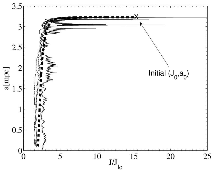
Figure 1.— Examples of tracks of stars from the MC simulation (solid lines), and a track from the effective model (dashed line) with $\xi=1$. The effective track represents the stochastic tracks well. The tracks extend to the point where $s\!=\!10^{-3}$. The relevant parameters are given in the first line of table (2), i.e. inspiral of a white dwarf into a MBH.

In this section we propose a heuristic analytical model, which captures some essential results of the MC simulations, while providing a more intuitive understanding.

In this model we define the equations of motion of an “effective track” of a star, which is deterministic and can be solved analytically. With this method we follow stars that start at some given initial semi-major axis $a_{0}$ and angular momentum $J_{0}$, and follow the star during its first two stages of inspiral, i.e., until the moment that $s\!<\!s_{\mathrm{crit}}$.

The DF of stars which reach $s\!=\!s_{\mathrm{crit}}$ is determined by the evolution of the orbital parameters ($J,a$) in the region where energy dissipation is efficient. Because of the strong dependence of the energy $\Delta E$ which is dissipated per orbit on angular momentum (or, equivalently, periapse), this is a small region $\Delta J$ in $J$-space, the size of which is of order of the loss-cone, $\Delta J\!\sim\!J_{lc}$. The time $\Delta t$ it typically takes a star with semi-major axis $a_{0}$ performing a random walk in $J$ to cross this region is $\Delta t\!=\![\Delta J/J_{m}(a_{0})]^{2}t_{h}$ ($t_{r}\!=\!t_{h}$ assumed). This can be used to introduce an effective $J$-“velocity” $\Delta J/\Delta t\!=\!-J_{m}^{2}(a_{0})/J_{lc}t_{h}$.

The effective velocity of the semi-major axis is given by

$$\frac{\mathrm{d}a(J,a)}{\mathrm{d}t}=\frac{da}{dE}\dot{E}=-\frac{2a^{2}}{GM_{\bullet}}\frac{\Delta E_{\mathrm{GW}}(J)}{P(a)}.$$ (43)

These two equation define a deterministic time evolution in ($J,a$) space from given initial values ($J(0)\!=\!J_{0},\,a(0)\!=\!a_{0}$), to a final point ($J_{f},a_{f}$), where $s\!=\!s_{\mathrm{crit}}$. To recover $W(J;a_{0})$ at $s_{\mathrm{crit}}$, we introduce some scatter in the effective velocities $\mathrm{d}J/\mathrm{d}t$,

$$\frac{\mathrm{d}j}{\mathrm{d}t}=-\xi y\frac{j_{m}^{2}(a_{0})}{t_{h}},$$ (44)

where $j$ denotes angular momentum in terms of $J_{lc}$, $y$ is drawn from the positive wing of the normalized Gaussian distribution, $G_{1}(y)$, and $\xi\!\sim\!1$ (a free parameter) is the width of the distribution, which can vary depending on the system’s parameters. Equations (43,44) can be solved analytically,

$$j(t)\!=\!j_{0}\!-\!y\xi j_{m}^{2}(a_{0})\frac{t}{t_{h}}\,,\qquad a(t)\!=\!\left[1\!-\!\frac{(d_{c}/a_{0})^{3/2}}{6\xi yj^{6}}\right]^{2}a_{0}\,.$$ (45)

The stopping condition $s(j,a)=s_{\textrm{crit}}$ gives an additional relation between $j$ and $a$, so that the final values are related by $a_{f}=s_{\mathrm{crit}}^{2/3}j_{f}^{-10/3}d_{c}.$ This ties the initial and final values through the equations of motions

$$y(j_{f})=\frac{(6\xi)^{-1}(d_{c}/a_{0})^{3/2}j_{f}^{-6}}{1-s_{\mathrm{crit}}^{1/3}(d_{c}/a_{0})^{1/2}j_{f}^{-5/3}}.$$ (46)

The relation between the initial distribution of $j$-velocities and the final $j$ distribution at is $W(j_{f};a_{0})=G_{1}(y)[\mathrm{d}y(j_{f})/\mathrm{d}j_{f}]\,.$ The integrated DF over all the cusp stars is

$$W(j_{f})\mathrm{d}j_{f}=\frac{\int^{a_{c}}N(a)W(j_{f};a)\,\mathrm{d}a}{\int^{a_{c}}N(a)\,\mathrm{d}a}\,.$$ (47)

4.4. Comparison of the different methods

We compare the results of the MC simulation, the diffusion-dissipation equation and an integration of equations (44) and (43). In all cases the calculation is stopped when $s\!=\!10^{-3}$; at that point the eccentricity is still approximately unity, but scattering becomes entirely negligible so that even in the MC simulation the quantities evolve essentially deterministically according to equations (20-24). The calculations assume a cusp with slope $p\!=\!0$, $M_{\bullet}\!=3\!\times\!10^{6}\,M_{\odot}$ and $M_{\star}\!=\!0.6$ (corresponding to WDs).

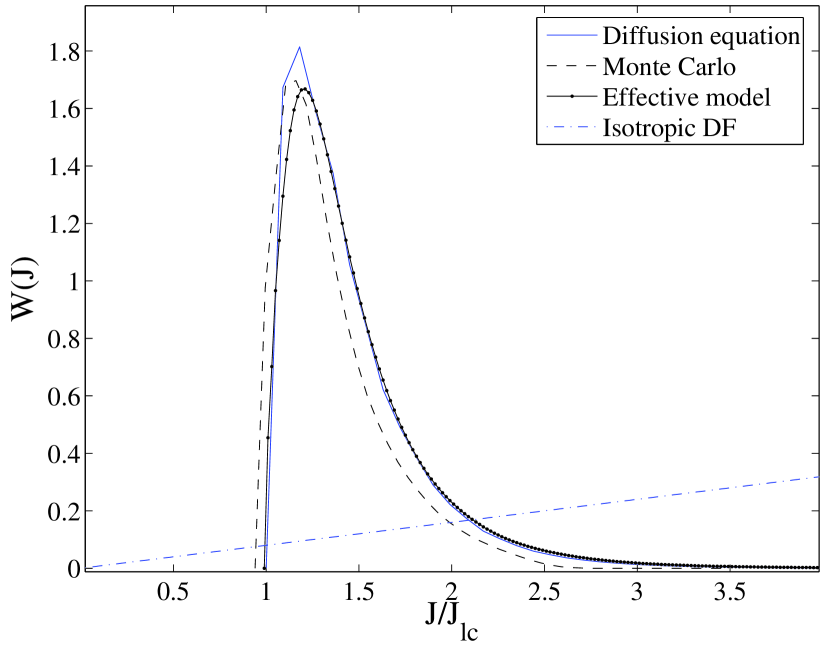
Figure 2.— A comparison of the DFs of angular momenta for inspiraling stars in a $p\!=\!0$ stellar cusp, derived from (1) MC simulations, (2) direct integration of the diffusion-dissipation equation (Eq. 42) and (3) the effective model (Eq. 47, with $\xi\!=\!0.6$). The DFs are normalized over the displayed $J$-range. The DFs are shown at $s\!=\!10^{-3}$, when the dynamics are dominated by dissipation and scattering no longer plays a role, but the orbits are still well outside the LISA band, $P\!\gg\!P_{L}$ and $e\!\rightarrow\!1$. This DF sets the initial conditions for the dissipation phase. The DF of the isotropic parent population (no sink, no dissipation; Eq. 9) is also shown for contrast. Unlike the DF of the inspiraling stars, it is dominated by high-$J$ stars.

Figure (2) shows the very good correspondence between the three approaches, whose underlying assumptions and approximations are summarized in table (1). One important conclusion is that all stars enter the dissipation phase with very small angular momenta, $1\!\lesssim\!J/J_{lc}\!\lesssim 2$. For a suitable choice of $\xi\!\sim\!1$, the actual complicated stochastic tracks are well mimicked by the tracks of the “effective stars”. The semi-analytical approach not only identifies the correct scale of angular momentum of inspiraling stars, but reproduces the DF. Its practical value lies in the relative ease of its application compared to the time consuming MC simulations or the integration of the diffusion-dissipation equation.

Table 1Comparison of assumptions in the 3 methods

Method	GR potential	$\Delta_{1}J_{{\rm scat}}$	$\Delta J_{{\rm GW}}$	Stop at $s_{{\rm crit}}$
Monte Carlo	yes	yes	yes	noa
Diffusion/Dissipation	no	no	no	yes
Effective track	no	no	no	yes
a For the purpose of comparison to the other two methods,
the MC simulation was terminated at $s_{\rm crit}$.

5. Inspiral rates and distribution of orbital parameters

We now proceed to apply the MC simulation to different types of COs inspiraling into a $3\!\times\!10^{6}\,M_{\odot}$ MBH in a galactic center, and into a $10^{3}\,M_{\odot}$ IBH in a stellar cluster. We find from the simulations the critical semi-major axis $a_{c}$ and calculate the DF of the eccentricities of LISA  sources. We stop the simulations when the orbital period falls below the longest period detectable by LISA  , $P_{L}\!=\!10^{4}\,\mathrm{s}$, which corresponds to a semi-major axis of

$$a_{L}=23.5M_{6}^{-2/3}r_{S},$$ (48)

where $M_{\bullet}=10^{6}M_{6}\,M_{\odot}$.We record the eccentricity at that point and construct the DF of the eccentricity at $P_{L}$. It is straightforward to integrate the orbits in the eccentricity histograms backward (forward) in time to larger (smaller) values of $P$, see e.g. Barack & Cutler (BC04a 2003).

The stars are distributed according to a powerlaw distribution with different values for $p$. The total number of stars within $r_{h}$ was assumed to be $N_{h}=2M_{\bullet}/M_{\odot}$, with different number fractions for the respective species. See table (2) for the assumed parameters of the stellar populations.

5.1. Massive black holes in galactic centers

We assume a $M_{\bullet}\!=\!3\!\times\!10^{6}\,M_{\odot}$ MBH as a representative example and make the simplifying assumption that the MBH is not spinning. Real MBHs probably have non-zero angular momentum (e.g. see for evidence of spin of the MBH in our Galactic Center Genzel et al. GS03 2003). An important qualitative difference is that in the Schwarzschild case the eccentricity of a GW-emitting star decreases monotonically with time, which this is not so for non-zero angular momentum (e.g. Glampedakis et al. GHK02 2002). We conducted several MC simulations with Kerr metric orbits and verified that in spite of changes in details, our overall results hold.

The tidal field of MBHs in this mass range disrupts main sequence stars before they can become detectable LISA sources. A possible exception is our own Galactic Center, where the weak GW emission from very low mass main sequence stars (which are the densest and so the most robust against tidal disruption) may be detected because of their proximity (Freitag FR03 2003). However, here we only consider GW from COs. Table (2) summarizes the parameters assumed for the properties of white dwarfs (WDs), neutron stars (NSs) and stellar mass black holes (BHs). The BHs are assumed to be strongly segregated in a steep cusp because of their much heavier mass (Bahcall & Wolf BW77 1977). The total (dark) mass in COs near MBHs is not known, but in future it may be constrained by deviations from Keplerian motions of luminous stars very near the MBH in the Galactic center (Mouawad et al. MO04 2004).

Table 2 Parameters for stellar populations and inspiral rates

Star	$M_{\star}$	$t_{h}$	$r_{h}$	$p$	$f_{s}$	$a_{c}^{c}$	$a_{c}^{d}$	$\Gamma_{i}$
	[$M_{\odot}$]	[Gyr]	[pc]			[mpc]	[mpc]	[$\mathrm{Gyr^{-1}}$]
WDa	0.6	$10$	2	0	$0.1$	30	20	7.8
NSa	1.4	$5$	2	0	0.01	40	20	1.8
BHa	10	$1$	2	1/4	$1(-3)$	20	10	4.7
NSb	1.4	$1(-3)$	0.05	0	0.01	2	1	4.3
BHb	10	$1(-3)$	0.05	1/4	1(-3)	5	2	6.7
a MBH with $M_{\bullet}\!=\!3\times 10^{6}\,M_{\odot}$
b IBH with $M_{\bullet}\!=\!10^{3}\,M_{\odot}$.
cFrom equation (30)
dFrom the MC simulations

Fig. (3) shows the normalized inspiral probability function $S_{s}(a_{0})$ , where $s$ stands for WD, NS, and BH. The critical semi-major axis is similar for WDs and NSs, but much smaller for BHs, because of the smaller relaxation time and the higher central concentration due to mass segregation. The functions $S_{s}(a)$ are used to calculate the inspiral rates (Eq. 17) that are listed in table (2). The rate for WDs is highest, $\Gamma_{\rm WD}=7.8\,{\rm Gyr^{-1}}$. We find that because of mass segregation, the rate for stellar BHs is of the same order of magnitude as that for WDs, $\Gamma_{\rm BH}=4.7\,{\rm Gyr^{-1}}$ although their number fraction is lower by two orders of magnitude. The hierarchy of rates in table (2) is not, of course, necessarily the same as cosmic rates that LISA will observe; NSs and BHs are more massive than WDs, and can be observed at larger distances.

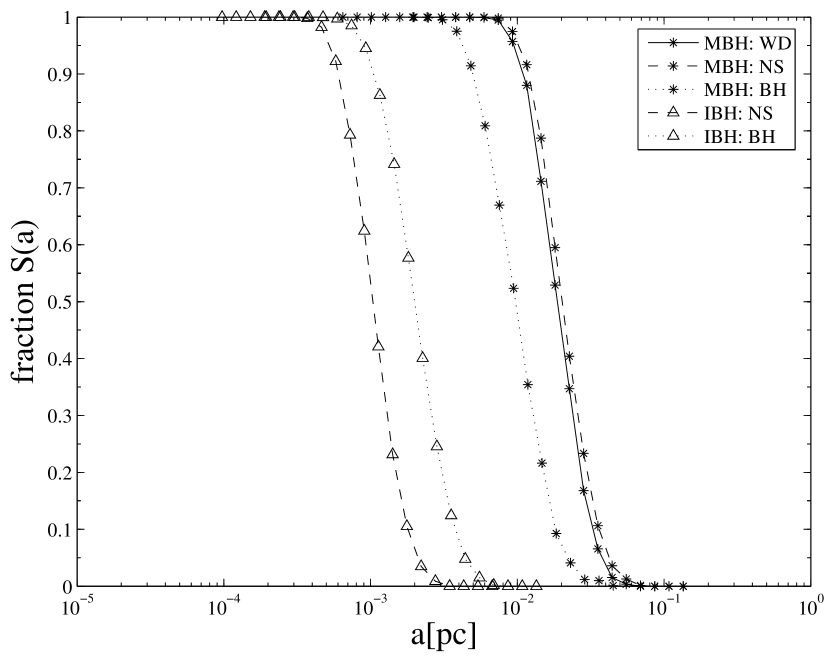
Figure 3.— Dependence of the normalized fraction of inspiral events on initial semi-major axis, for the case of a MBH of $M_{\bullet}\!=\!3\times 10^{6}\,M_{\odot}$ (asterisks) and an IBH (triangles). The solid line is for white dwarfs, the dashed lines for neutron stars, and the dotted lines for stellar mass black holes. For the parameters of these cases see table (2).

Fig. (4) shows the eccentricity DFs of stars on orbits with $P\!=\!P_{L}$; note that since $a\!=\!a_{L}$ is fixed, the orbits are fully determined by $e$. The DFs show a strong bias to large eccentricities. The maximal eccentricity possible for a star orbiting a $3\!\times\!10^{6}\,M_{\odot}$ MBH in the LISA band is $e_{\textrm{max}}\!=\!0.81$ (Eq. 39).

It should be emphasized that the histogram in figure (4) can be obtained deterministically from the DF $W(J;s_{\mathrm{crit}}\!=\!10^{-3})$ in figure (2), because the stars have already reached the point where scattering is negligible. This would not be the case had the MC simulation been terminated at $s_{\mathrm{crit}}=1$ (e.g. Freitag FR03 2003), since then significant scatterings would continue to redistribute the orbital parameters. We find however that the final DF (at $P\!=\!P_{L}$), which is obtained by integrating $W(J;s_{\mathrm{crit}}\!=\!1)$ forward in time according to the GW dissipation equations (Eqs. 20,23) without scattering, is not much different from that shown in Fig. (4). This coincidence is due to the fact that the stars with the largest eccentricities, which typically drop into the MBH, are replenished by the stars with slightly lower eccentricities. The main consequence of choosing $s_{\mathrm{crit}}$ too large is an overestimate of the total event rate; stars which actually fall into the MBH are erroneously counted as contributing to the GW event rate. Incidentally, even though stars that do not complete the inspiral are not individually resolvable, they will contribute to the background noise in the LISA band (Barack & Cutler BC04b 2004).

A premature neglect of the effects of scattering in previous studies (e.g. Freitag FR01 2001) probably explains in part why our derived rates are significantly lower. Those studies usually assumed that stars will spiral in without further perturbations once $s\!=\!1$. We ran a simulation that was stopped at $s_{\mathrm{crit}}\!=\!1$ instead of $s_{\mathrm{crit}}\!=\!10^{-3}$. The event rate in that unrealistic case is about $\sim\!6$ times higher. This does not explain all of the discrepancies, which are hard to track as different methods are used. The different stopping criterion may also explain why our rates are lower than those estimated by Hils & Bender (HB95 1995), who used a method similar to ours, without specifying the criterion for inspiral.

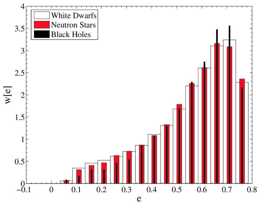
Figure 4.— The probability DF of a CO entering the LISA band with eccentricity $e$ for a MBH of mass $M_{\bullet}\!=\!3\!\times\!10^{6}\,M_{\odot}$. The histograms represent WDs, NSs and BH (from broad to narrow). Note that the maximal possible eccentricity for which $P\!<\!P_{L}$ is $e_{\textrm{max}}\!=\!0.81$. See table (2) for the cusp parameters.

5.2. Intermediate mass black holes in stellar clusters

Unlike MBHs with masses $M_{\bullet}\!\gtrsim\!10^{6}\,M_{\odot}$ , there is little firm observational evidence at this time for the existence of IBHs with masses $M_{\bullet}\!\sim\!10^{3}\,M_{\odot}$ (see review by Miller & Colbert MC04 2004). However, there are plausible arguments arguing in favor of their existence. From a theoretical point of view, these objects are thought to form naturally, such as in population III remnants (Madau & Rees MR01 2001), or in a runaway merger of young stars in dense stellar clusters (Portegies Zwart & McMillan PZM01 2001; Portegies Zwart et al. PZea04 2004). From an observational perspective, IBHs may power some of the ultraluminous X-ray sources (e.g. Miller, Fabian, & Miller MFM04 2004), for example by tidal capture of a main sequence companion star (Hopman et al. HPZA04 2004).

For the purpose of estimating the orbital parameters of GW emitting stars, we assume that IBHs lie at the center of dense stellar clusters (see model parameters listed in table 2). White dwarfs are disrupted by an IBH before entering the LISA band, so that only the most compact sources, neutron stars and stellar mass BHs can emit GW in the LISA frequency band. The same values for the stellar population fractions $f_{s}$ where taken here as for MBHs. We note that this is not necessarily the case. For example, N-body simulations indicate that a large fraction of BHs may be ejected in an early stage of the cluster’s life if a massive stellar object forms a tight binary with the IBH (Baumgardt et el. 2004b ).

Figure (3) shows the inspiral probability functions $S_{s}(a)$, and Fig. (5) shows the eccentricity histograms of stars on orbits with $P=P_{L}$. The maximum eccentricity still observable by LISA is nearly unity, and the IBH case shows even more clearly the strong tendency towards large eccentricities. In general, this effect becomes more prominent for lighter BHs. The high eccentricity makes the GW signal highly non-monochromatic. The star spends most time at apo-apse, emitting a relatively weak, low frequency signal. At periapse short pulses of high frequency GW is emitted. For IBHs of $M_{\bullet}\!\sim\!10^{3}\,M_{\odot}$, the frequency $\nu_{p}$ of these short bursts at periapse is of the order $\nu_{p}\lesssim 100$ Hz. This is too high to be measurable by LISA , but may be measurable by ground based detectors such as LIGO or VIRGO.

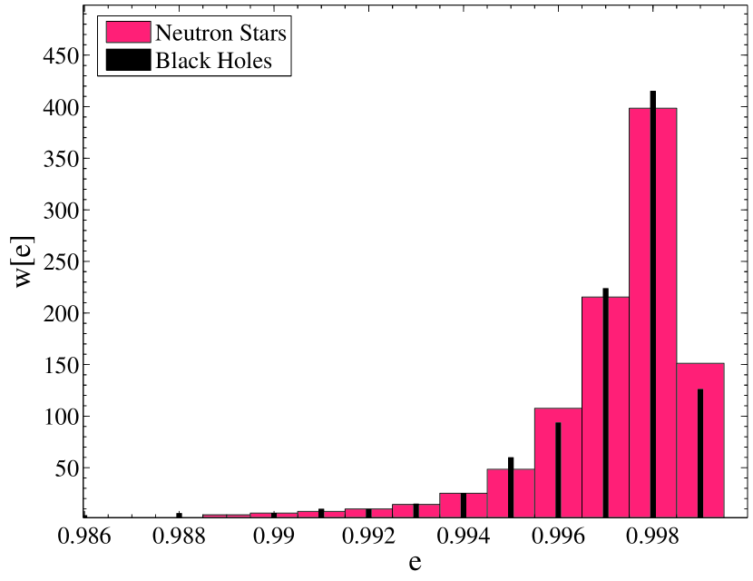
Figure 5.— The probability DF of a compact remnant entering the LISA band with eccentricity $e$ for an IBH of mass $M_{\bullet}\!=\!10^{3}\,M_{\odot}$. Only NSs (broad) and BHs (narrow) are considered; WDs are probably disrupted by the tidal field. For an IBH, the maximal possible eccentricity for which $P\!<\!P_{L}$ is nearly unity, $e_{\textrm{max}}\!=\!0.998$, all inspiraling stars are likely to have eccentricities close to the maximum value. See table (2) for the cusp parameters.

As anticipated (Eq. 35), the rate of inspiraling stars is comparable to that of a MBH (Table 2). However, due to the extremely high eccentricities and small semi-major axes of the orbits, the GW emission is very efficient and they spiral in on a very short time scale (on the order of a year).

6. Summary and discussion

Stars spiraling into MBH due to the emission of GW are an important potential source for future GW detectors, such as LISA. The detection of the signal against the noise will be challenging, and requires pre-calculated wave-forms. The waveforms depend on the orbital parameters of the inspiraling stars. Our main goal in this study was to derive the distribution of eccentricities of inspiraling stars. The orbital statistics of such stars reflect a competition between orbital decay through dissipation by the emission of GW, and scattering, which deflects stars into eccentric orbits but can also deflect them back to wider orbits or straight into the MBH.

Inspiral is a slow process, and unless the stars start close enough to the MBH, they will be scattered off their orbit. We identified a critical length scale $a_{c}$ which demarcates the volume from which inspiral is possible. We obtained an analytical expression for the inspiral rate and showed that it is of the order of a few per Gyr per galaxy, much smaller than the rate for direct capture (Alexander & Hopman AH03 2003), that it is nearly independent of the relaxation time for typical stellar cusps, and that it grows slowly with decreasing MBH mass (assuming the $M_{\bullet}-\sigma$ relation). Throughout we assumed a single powerlaw DF. Generalization to different profiles is straightforward. Qualitatively, the inspiral rate is determined by the stellar density near $a_{c}$, and is not very sensitive to the exact profile far away at radii much smaller or much larger than $a_{c}$. The rate of GW events depends on the number of COs inside $a_{c}$ (which is much smaller than the MBH radius of influence), and so mass-segregation can play an important role in enhancing the event rate by leading to a centrally concentrated distribution of COs.

We obtained a relatively low rate. One important reason for this is our stringent criterion for inspiral. This may also explain why our results deviate from Hils & Bender HB95 1995, although they do not specify their precise criterion for inspiral. Comparison with other works are more complicated. Possible differences may stem from different normalizations of the central density, different CO fractions, different criteria for inspiral, and the way mass segregation is treated. An essential step in the future will be to analyze inspiral processes by N-body simulations, which are feasible already for small systems (Baumgardt et al. 2004a , 2004b ; Preto et al. P04 2004).

The detection rate depends on the inspiral rates, but also on the mass, relaxation time, the orbital parameters (especially the eccentricity) and the details of the detection algorithm (Barack & Cutler BC04a 2003). Here we provide a simple recipe to estimate the number of detectable sources. We assume that the various dependencies above can be expressed by an effective strain $\hat{h}$.

The strain of GW resulting from a star of mass $M_{\star}=mM_{\odot}$ orbiting a MBH of mass $M_{\bullet}=10^{6}M_{\odot}M_{6}\gg M_{\star}$ at a distance $d={\rm Gpc}\,d_{\rm Gpc}$, on a circular orbit of orbital frequency $\nu=10^{-3}{\rm s^{-1}}\nu_{-3}$, is given by

$$h=1.7\times 10^{-23}\nu_{-3}^{2/3}d_{\rm Gpc}^{-1}M_{6}^{2/3}m.$$ (49)

(e.g., Sigurdsson & Rees SR97 1997).

The cosmic rate of LISA events is given by

$$\Gamma_{\rm tot}=\int_{M_{\rm min}}^{M_{\rm max}}dM_{\bullet}{dn_{\bullet}\over dM_{\bullet}}\Gamma_{i}(M_{\bullet})V(M_{\bullet}),$$ (50)

where $dn_{\bullet}/dM_{\bullet}$ is the number of MBHs per unit mass, per unit volume, and $V(M_{\bullet})$ is the volume in which stars can be observed by LISA. Aller & Richstone (AR02 2002) used the $M_{\bullet}-\sigma$ relation to “weigh” the MBHs. The spectrum is roughly approximated by

$${dn_{\bullet}\over dM_{\bullet}}=10^{7}\left({1\over 10^{6}M_{\odot}}\right)M_{6}^{-1}\,{\rm Gpc^{-3}}.$$ (51)

The LISA sensitivity curve at $\nu=10^{-3}$ is $h\sim 10^{-23}$ for one year of observation with signal to noise ratio S/N=1 (see e.g. http://www.srl.caltech.edu/lisa). We adopt this value as a representative detection threshold for $\hat{h}$. If the effective strain has to be be at least $10^{-23}\hat{h}_{-23}$ for the star to be observable, then, for a Euclidean Universe,

$$V(M_{\bullet})=20.6\,{\rm Gpc^{3}}\,\hat{h}_{-23}^{-3}\nu_{-3}^{2}m^{3}M_{6}^{2}.$$ (52)

Finally, the rate per MBH is

$$\Gamma_{i}(M_{\bullet})=\Gamma_{i}(3\times 10^{6}M_{\odot})(3M_{6})^{-1/4},$$ (53)

where we used the expression for the dependence of the inspiral rate on the MBH mass, equation (35), with $\beta=4$. The expression can be calibrated with the MC results for a $3\times 10^{6}M_{\odot}$ MBH.

Integrating (50) from $M_{6}=0.5$ to $M_{6}=5$ gives

$$\Gamma_{\rm tot}=1.5\,{\rm yr^{-1}}\,\left[{\Gamma_{i}(3\times 10^{6}M_{\odot})\over{\rm Gyr^{-1}}}\right]m^{3}\hat{h}_{-23}^{-3}\nu_{-3}^{2}.$$ (54)

The number of sources which LISA can observe at any moment is estimated by $\mathcal{N}=\Gamma_{\rm tot}\times t_{L}(\bar{e},a_{L})$, where $t_{L}$ is the time a star with eccentricity $\bar{e}$ spends in the LISA band before being swallowed; here $\bar{e}$ is the average eccentricity of stars entering the LISA band.

For example, our calculations for WD inspiral indicate that $\Gamma_{i}(3\times 10^{6}M_{\odot})=7.8\,{\rm Gyr^{-1}}$. For a circular orbit with a period of $P=10^{3}\,{\rm s}$ and $M_{6}=1$, the inspiral time is $t_{L}=54\,{\rm yr}$, in which case the number of detectable sources would be $\mathcal{N}\sim\,130\hat{h}_{-23}^{-3}\nu_{-3}^{2}$.

We would like to emphasize that this estimate is to be treated with caution. The number of detectable sources depends strongly on the assumptions. In particular, GWs from eccentric sources are not monochromatic and may be harder to detect. The analysis in this paper can be used for a more detailed analysis of the number of detectable LISA sources.

We used three complementary methods to model the inspiral process, MC simulations, numerical solution of the diffusion/dissipation equation and an analytic effective orbit model. We followed the evolution of the orbital properties of the inspiraling stars to the point where they decoupled from the scattering. All three methods were in excellent agreement. We find that the distribution of orbital angular momenta is strongly peaked near $J\!\gtrsim\!J_{lc}$, with the detailed form of the distribution depending somewhat on the parameters of the stellar system. We demonstrated that estimates that “freeze” the scattering prematurely may lead to erroneously high rates by counting stars that actually plunge into the MBH. We then used the most versatile method, the MC simulations, to continue evolving the orbits in a GR Schwarzschild potential, taking into account energy and angular momentum loss due to GW emission (and residual perturbations by scattering). We derived the distribution of eccentricities of the inspiraling stars as they enter the detection window (orbital period of $P_{L}\!\lesssim\!10^{4}\,\mathrm{s}$ for LISA).

Our main result is that the eccentricities of stars entering the LISA band are strongly skewed toward high values.

References

- 1 Alexander, T., 1999, ApJ, 520, 137
- 2 Alexander, T., & Morris, M., 2003, ApJ, 590, L25
- 3 Alexander, T., & Hopman, C., 2003, ApJ, 590, L29
- 4 Aller, M. C., & Richstone, D., 2002, AJ, 124, 3035
- 5 Bahcall, J. N., & Wolf, R. A., 1976, ApJ, 209, 214
- 6 Bahcall, J. N., & Wolf, R. A., 1977, ApJ, 216, 883
- 7 Barack, L., & Cutler, C., 2004, PRD, 69, 082005
- 8 Barack, L., & Cutler, C., 2004, gr-qc/0409010
- 9 Baumgardt, H., Makino, J., & Ebisuzaki, T., 2004a, ApJ, 613, 1133
- 10 Baumgardt, H., Makino, J., & Ebisuzaki, T., 2004b,ApJ, 613, 1143
- 11 Binney, J. & Tremaine, S., 1987, Galactic Dynamics (Princeton: Princeton Univ. Press)
- 12 Cohn, H., & Kulsrud, R. M. 1978, ApJ, 226, 1087
- 13 Cutler, C., Kennefick, D., & Poisson, E., 1994, PRD, 50, 6
- 14 Ferrarese, L., & Merritt, D., 2000, ApJ, 539, L9
- 15 Figer, D. F., Kim, S. S., Morris, M., Serabyn, E., Rich, R. M., & McLean, I. S. 1999, ApJ, 525, 750
- 16 Frank, J., & Rees, M. J., 1976, MNRAS, 176, 633
- 17 Freitag, M., & Benz, W, 2001, A&A, 375, 711
- 18 Freitag, M., 2001, Class. Quantum Grav., 18, 4033
- 19 Freitag, M., 2003, ApJ, 583, L21
- 20 Freitag, M. & Benz, W., 2002, A&A, 394, 345
- 21 Gair, J. R., Barack, L., Creighton, T., Cutler, C., Larson, S., L., Phinney, E. S., Vallisneri, M., 2004, gr-qc/0405137
- 22 Gebhardt, K., et al., 2000, ApJ, 539, L13
- 23 Gebhardt, K., et al. 2003, ApJ, 583, 92
- 24 Genzel, R. et al., 2003, ApJ, 594, 812
- 25 Genzel, R., Schödel, R., Ott, T., Eckart, A., Alexander, T., Lacombe, F., Rouan, D., & Aschenbach, B., 2003, Nature, 425, 934
- 26 Glampedakis, K., Hughes, S. A., & Kennefick, D., 2002, Phys. Rev. D, 66, 064005
- 27 Hils, D., & Bender, P. L., 1995, ApJ, 445, L7
- 28 Hopman, C., Portegies Zwart, S.F., & Alexander, T., 2004, ApJ, 604, L101
- 29 Ivanov, P. B., 2002, MNRAS, 336, 373, 2002
- 30 Lightman, A. P., & Shapiro, S. L., 1977, ApJ, 211, 244
- 31 Madau, P., & Rees, M. J., 2001, ApJ551, L27
- 32 Magorrian, J., & Tremaine, S., 1999, MNRAS, 309, 447
- 33 Miller, M. C., & Colbert, J. M., 2004, Int.J.Mod.Phys. D13 1-64
- 34 Miller, J. M., Fabian, A., C., & Miller, M. C., 2004, 614, ApJ, L117
- 35 Miralda-Escudé, J., & Gould, A., 2000, ApJ, 545, 847
- 36 Mouawad, N., Eckart, A., Pfalzner, S., Schödel, R., Moultaka, J., Spurzem, R., 2004, Astronomische Nachrichten, Vol. 326, 2, 83-95
- 37 Peebles, P. J. E., 1972, ApJ, 178, 371
- 38 Peters, P. C. 1964, Phys. Rev., 136, 1224
- 39 Pierro, V., Pinto, I. M., Spallicci, A. D., Laserra, E., Recano, F., 2001, MNRAS, 325, 358
- 40 Portegies Zwart, S. F., McMillan, S. L. W. 2002, ApJ, 576, 99
- 41 Portegies Zwart, S. F., Baumgardt, H., Makino, J., McMillan, S. L., & Hut, P., Nature, 428, 724
- 42 Press, W. H., Teukolsky, S. A., Vetterling, W. T., & Flannery, B. P. 1992, (Cambridge: University Press), 2nd ed.
- 43 Preto, M., Merritt, D., Spurzem, R., 2004, ApJ, 613, L109
- 44 Quinlan, G. D., Hernquist, L., & Sigurdsson, S., 1995, ApJ, 440, 554
- 45 Sigurdsson, S., astro-ph/0304251
- 46 Sigurdsson, S., and Rees, M. J., 1997, MNRAS284, 318
- 47 Syer, D., & Ulmer, A., 1999, MNRAS, 306, 35
- 48 Tremaine, S., et al., 2002, ApJ, 574, 740
- 49 Wang, J., & Merritt, D., 2004, ApJ, 600, 149
- 50 Wen & Gair, 2005, pre-print: gr-qc/0502100
- 51 Young, P., 1980, ApJ, 242, 1232
- 52 Zhao, H.-S., Haehnelt, M. G., & Rees, M. J., 2002, New Astron., 7, 385