Quantum corrections to slow roll inflation and new scaling of superhorizon fluctuations.

Abstract

Precise cosmological data from WMAP and forthcoming cosmic microwave background experiments motivate the study of the quantum corrections to the slow roll inflationary parameters. We find the quantum (loop) corrections to the equations of motion of the classical inflaton, to those for the fluctuations and to the Friedmann equation in general single field slow roll inflation. We implement a renormalized effective field theory (EFT) approach based on an expansion in $\left(H/M_{Pl}\right)^{2}$ and slow roll parameters $\epsilon_{V},\;\eta_{V},\;\sigma_{V},\;\xi_{V}$. We find that the leading order quantum corrections to the inflaton effective potential and its equation of motion are determined by the power spectrum of scalar fluctuations. Its near scale invariance introduces a strong infrared behavior naturally regularized by the slow roll parameter $\Delta=\eta_{V}-\epsilon_{V}=\frac{1}{2}(n_{s}-1)+r/8$. To leading order in the (EFT) and slow roll expansions we find $V_{eff}(\Phi_{0})=V_{R}(\Phi_{0})\left[1+\frac{\Delta^{2}_{\mathcal{T}}}{32}\frac{n_{s}-1+\frac{3}{8}\;r}{n_{s}-1+\frac{1}{4}\;r}+\textmd{higher orders}\right]$ where $n_{s}$ and $r=\Delta^{2}_{\mathcal{T}}/\Delta^{2}_{\mathcal{R}}$ are the CMB observables that depend implicitly on $\Phi_{0}$ and $V_{R}(\Phi_{0})$ is the renormalized classical inflaton potential. This effective potential during slow roll inflation is strikingly different from the usual Minkowski space-time result. We also obtain the quantum corrections to the slow roll parameters in leading order. Superhorizon scalar field fluctuations grow for late times $\eta\to 0^{-}$ as $|\eta|^{-1+\Delta-d_{-}}$ where $d_{-}$ is a novel quantum correction to the scaling exponent related to the self-decay of superhorizon inflaton fluctuations $\varphi\rightarrow\varphi\varphi$ and $\eta$ is the conformal time. We find to leading order $-d_{-}=\Delta_{\mathcal{R}}^{2}\frac{\sigma_{V}\;(\eta_{V}-\epsilon_{V})+6\,\xi^{2}_{V}}{4\,(\eta_{V}-\epsilon_{V})^{2}}$ in terms of the CMB observables. These results are generalized to the case of the inflaton interacting with a light scalar field $\sigma$ and we obtain the decay rate $\Gamma_{\varphi\rightarrow\sigma\sigma}$. These quantum corrections arising from interactions will compete with higher order slow-roll corrections in the gaussian approximation and must be taken into account for the precision determination of inflationary parameters extracted from CMB observations.

I Introduction

Inflation is a central part of early Universe cosmology passing many observational tests and becoming a predictive scenario scrutinized by current and forthcoming observations. Originally, inflation was introduced as an elegant explanation for several shortcomings of the standard Big Bang cosmologyguth -riottorev . However, one of the most compelling aspects of inflation is that it provides a mechanism for generating scalar (density) and tensor (gravitational wave) perturbationsmukhanov -bran . A distinct aspect of inflationary perturbations is that these are generated by quantum fluctuations of the scalar field(s) that drive inflation. After their wavelength becomes larger than the Hubble radius, these fluctuations are amplified and grow, becoming classical and decoupling from causal microphysical processes. Upon re-entering the horizon, during the matter era, these classical perturbations seed the inhomogeneities which generate structure upon gravitational collapsemukhanov -bran . While there is a great diversity of inflationary models, most of them predict fairly generic features: a gaussian, nearly scale invariant spectrum of (mostly) adiabatic scalar and tensor primordial fluctuations. These generic predictions of most inflationary models make the inflationary paradigm fairly robust. The gaussian, adiabatic and nearly scale invariant spectrum of primordial fluctuations provide an excellent fit to the highly precise wealth of data provided by the Wilkinson Microwave Anisotropy Probe (WMAP)komatsu ; spergel ; kogut ; peiris . Perhaps the most striking validation of inflation as a mechanism for generating superhorizon (‘acausal’) fluctuations is the anticorrelation peak in the temperature-polarization (TE) angular power spectrum at $l\sim 150$ corresponding to superhorizon scaleskogut ; peiris .

The confirmation of many of the robust predictions of inflation by current high precision cosmological observations is placing inflationary cosmology on solid grounds. Current and forthcoming observations with ever increasing precision measurements will begin to discriminate among different inflationary models, placing stringent constraints on the underlying particle physics model of inflation. There are small but important telltale discriminants amongst different models: non-gaussianity, a running spectral index for either scalar or tensor perturbations (or both), an isocurvature component for scalar perturbations, different ratios for the amplitudes between scalar and tensor modes, etc. Already WMAP reports a hint of deviations from constant scaling exponents (running spectral index)peiris . Amongst the wide variety of inflationary scenarios, slow roll inflationbarrow ; stewlyth provides an appealing, simple and fairly generic description of inflation. The basic premise of slow roll inflation is that the potential is fairly flat during the inflationary stage. This flatness not only leads to a slowly varying Hubble parameter, hence ensuring a sufficient number of e-folds, but also provides an explanation for the gaussianity of the fluctuations as well as for the (almost) scale invariance of their power spectrum. A flat potential precludes large non-linearities in the dynamics of the fluctuations of the scalar field, which is therefore determined by a gaussian free field theory. Furthermore, because the potential is flat the scalar field is almost massless, and modes cross the horizon with an amplitude proportional to the Hubble parameter. This fact combined with a slowly varying Hubble parameter yields an almost scale invariant primordial power spectrum. Upon crossing the horizon the phases of the quantum fluctuations freeze out and a growing mode dominates the dynamics, i.e. the quantum fluctuations become classical (see ref.liddle and references therein). Departures from scale invariance and gaussianity are determined by the departures from flatness of the potential, namely by derivatives of the potential with respect to the expectation value of the scalar field. These derivatives can be combined into a hierarchy of dimensionless slow roll parametersbarrow that allow an assessment of the corrections to the basic predictions of gaussianity and scale invarianceliddle . This slow roll expansion has the important bonus of allowing a reconstruction program that yields details of the inflaton potential from observables extracted from the analysis of CMB data, for example the index of the power spectra of scalar and tensor perturbations, the ratio of their amplitudes, etc.lidsey . While more complicated scenarios can be proposed, the current WMAP data seems to validate the simpler slow roll scenariopeiris . Forthcoming precision CMB data forces a deeper examination of the inflationary predictions, which has motivated an analysis of the power spectra to higher order in the slow roll expansion. A general slow roll approximationstewart ; domi along with WKBmartin ; casa and uniformsalman approximations to study the power spectrum beyond slow roll have been introduced. While progress is being made in obtaining a more precise assessment of the power spectra of scalar and tensor perturbations within the slow roll scenario, it must be noted that all these refinements are still within the gaussian approximation, namely quadratic fluctuations of the scalar field and the metric (or alternatively linear perturbations in the equations of motion for the fluctuations). Interactions of the inflaton with other fields are a necessary ingredient for a post-inflationary reheating stage where the energy stored in the inflaton is transferred to other degrees of freedom which eventually thermalize and lead to a transition from inflation to the standard Hot Big Bang, radiation dominated cosmology.

Even within the simple single field slow roll scenario, higher derivatives of the potential with respect to the homogeneous expectation value of the scalar field will unavoidably lead to non-linearities. The lowest order non-linearity results from a cubic self-interaction of the fluctuations around the homogeneous expectation value. The strength of the cubic self-interaction is determined by a particular slow-roll parameter, (the ‘jerk’ parameter)liddle ; lidsey ; peiris . This slow roll parameter also enters in the running of the spectral index, and the current WMAP data provides a rather loose bound on itpeiris which suggests a small but non-vanishing cubic self-interaction.

Self-interactions of the fluctuations of the scalar field in turn lead to non-gaussianities which are characterized by a non-vanishing bi-spectrumallen -7L . The effect of interactions on the decay of the inflaton in de Sitter space time was studied in refs.prem , and we have implemented a dynamical renormalization group to study the decay of the quantum fluctuations into other fields as well as the self decay of the fluctuations both for sub and super-horizon modes in slow roll inflationultimonuestro1 ; ultimonuestro2 . Inultimonuestro2 the connection between the self-decay of inflaton fluctuations and the bi-spectrum in single field slow roll inflation was established.

In this article we study the effect of the self interactions as well as the interaction of the inflaton with other scalar fields to assess the quantum corrections to the potential reconstruction program based on the slow-roll expansion. In particular, we study the quantum corrections to the equations of motion of the expectation value of the inflaton, and to the fluctuations as well as the quantum corrections to the Friedmann equation and to the slow roll parameters. Such corrections are important for an accurate assessment of the inflationary parameters fit from the WMAP and future CMB data.

Inflation as an effective field theory: Effective field theory provides a useful and physically motivated interpretation of scalar field inflation below a cutoff scale. In this interpretation, inflation is driven by a scalar field (the inflaton) with a fairly flat potential, which justifies the slow roll approximation and is consistent with observational data. The inflaton replaces the microscopic description provided by grand unified models in the cosmological space-time. Such a description as an effective field theory relies on a separation of scales, in this case the scale of inflation, determined by the Hubble parameter, and a high energy scale $M$. We identify $M$ with the Planck scale $M_{Pl}$ since so far, this is the only known energy scale above the inflation scale. Within this effective field theory approach to inflationary cosmology the inflaton model is interpreted as the effective ‘low energy’ field theory resulting from ‘integrating out’ the degrees of freedom with energy scales at or even above the scale $M$ (as advocated in refs.kalohol ). In this interpretation, inflationary models are not fundamental theories but effective descriptions in terms of a condensate, the inflaton field. This type of description is very successful in a wide variety of physically relevant cases: the low energy pion dynamics emerging from full QCD and the Landau-Ginzburg effective theories of superconductivity, superfluidity and critical phenomena. In all these cases the low energy effective field theory allows a systematic study of the universal aspects of the relevant dynamics. In this approach small dimensionless quantities are a result of the ratio between the low and high energy scales. It is a tantalizing possibility that the robustness of the predictions of inflationary theories may be a manifestation of such ‘universality’ of the low energy effective field theory, akin to the robustness of the description of critical phenomena by the Landau-Ginsburg approach to phase transitions. Such point of view for inflationary dynamics as an effective field theory driven by a scalar field has been recently studied quantitatively in ref.hector .

The small parameter that determines the validity of inflation as an effective quantum field theory below the scale $M$ is $H/M$ where $H$ is the Hubble parameter during inflation and therefore the scale at which inflation occurs. The slow roll expansion is in a very well defined sense an adiabatic approximation since the time evolution of the inflaton field is slow on the expansion scale. Thus the small dimensionless ratio $H/M$, which is required for the validity of an effective field theory (EFT) is logically independent from the small dimensionless combinations of derivatives of the potential which ensure the validity of the slow-roll expansion. In particular, since $M=M_{Pl}$, the ratio $H/M_{Pl}$ determines the amplitude of tensor perturbationsliddle . Hence the validity of the effective field theory description of inflation requires a very small amplitude of tensor perturbations (gravitational waves) which is consistent with the WMAP datapeiris .

Therefore, in this article we will invoke two independent approximations, the effective field theory (EFT) and the slow roll approximation. The former is defined in terms of an expansion in the ratio $H/M_{Pl}$, whereas the latter corresponds to small slow roll parameters.

In order to determine the validity of the (EFT) and slow roll expansions, it is important to highlight the main differences between slow roll inflation and the post-inflationary stage. During slow roll inflation the dynamics of the scalar field is slow on the time scale of the expansion and consequently the change in the amplitude of the inflaton is small and quantified by the slow roll parameters. The slow roll approximation is indeed an adiabatic approximation. In striking contrast to this situation, during the post-inflationary stage of reheating the scalar field undergoes rapid and large amplitude oscillations that cannot be studied in a perturbative expansionreheatnuestro ; ramsey . The slow roll approximation during inflation is warranted because of the adiabatic evolution of the scalar field, and the (EFT) is warranted because of the smallness of the ratio $H/M_{Pl}$ as determined by the WMAP data.

The goals of this article: In our previous work in ref.ultimonuestro1 ; ultimonuestro2 we have found that the near scale invariance of the inflaton fluctuations result in quantum corrections that feature an infrared enhancement.

The results of these references suggest that even when quantum (loop) corrections are suppressed by powers of the effective field theory ratio $H/M_{Pl}$, there are enhancements arising from infrared effects, a result of the near scale invariance of the power spectrum of fluctuations.

In this article we focus our study on quantum aspects of inflationary dynamics during the slow roll stage by considering quantum (loop) corrections from inflaton fluctuations as well as light scalar fields with a nearly scale invariant power spectrum. In particular we study the contributions from the inflaton fluctuations and light scalar fields to the effective inflaton potential as well as self-energy corrections to the equations of motion of the inflaton fluctuations during slow roll. We show that a strong infrared enhancement appears in the effective field theory when nearly scale invariant fluctuations are present. This is precisely the case in slow-roll inflationary cosmology.

We restrict our study here to the quantum corrections from fluctuations of the inflaton and light scalar fields during slow roll as a prelude to a more complete study that should eventually include gravitational fluctuations, a task that is postponed for further study.

The motivation of this work is driven by forthcoming precision measurements of the primordial power spectrum. These measurements can potentially yield precise information to map out the inflationary potential during inflation. In order to go from the data to the inflaton potential and inflationary parameters, the slow-roll approximation is typically invoked. Higher order derivatives of the inflationary potential will be determined from the slow roll parameters obtained from the data. The main point that we highlight in this article is that while the typical slow-roll expansion is based solely on a free field description (gaussian) of the fluctuations and a classical description of the inflaton dynamics, quantum (loop) corrections yield contributions in the slow-roll parameters. These quantum corrections compete with higher order corrections in the slow roll approximation in the gaussian theory and therefore affect the determination of the inflationary potential. Our study in this article seeks to obtain a quantitative understanding of these corrections. We find that the loop corrections have a strong infrared behavior as a consequence of the nearly scale invariant spectrum of scalar fluctuations. The infrared behavior is manifest as poles in a small parameter $\Delta$ which is a measure of the departure from scale invariance of the power spectrum of scalar perturbations. $\Delta$ is a simple function of slow-roll parameters.

Brief summary of main results:

• We show that the one loop quantum correction to the equation of motion for the homogeneous expectation value of the inflaton is determined by the power spectrum of its quantum fluctuations. As discussed inultimonuestro2 , a nearly scale invariant power spectrum of scalar fluctuations introduces a strong infrared behavior: it is naturally regulated by a small parameter $\Delta$ which measures the departure from scale invariance and is a simple function of slow-roll parameters. The infrared divergences are manifest as poles in $\Delta$ultimonuestro2 . We obtain the effective equation of motion for the expectation value of the inflaton field at one loop level in the effective field theory and to leading order in the slow roll expansion. It is given by

  $$\ddot{\Phi}_{0}(t)+3\,H_{0}\,\dot{\Phi}_{0}(t)+V^{{}^{\prime}}_{R}(\Phi_{0})\left\{1+\frac{\Delta_{\mathcal{R}}^{2}}{n_{s}-1+\frac{r}{4}}\left[\frac{r}{2}\left(n_{s}-1+\frac{3\,r}{16}\right)-\frac{dn_{s}}{d\ln k}\right]\right\}=0\;.$$

• We obtain the one-loop corrections to the Friedmann equation to leading order in the EFT and slow roll expansions. Just as for the equation of motion for the expectation value of the inflaton, the one-loop correction to the Friedmann equation is determined by the power spectrum of the inflaton fluctuations and also features an infrared enhancement. The effective inflaton potential is obtained to leading order in the EFT and slow roll approximations, it is given by

  $$V_{eff}(\Phi_{0})=V_{R}(\Phi_{0})\left[1+\frac{r\;\Delta^{2}_{\mathcal{R}}}{32}\;\frac{n_{s}-1+\frac{3}{8}\;r}{n_{s}-1+\frac{1}{4}\;r}\right]\;.$$

  where the CMB observables $n_{s}\,,\,r$ are implicit functions of $\Phi_{0}$ through the slow roll parameters. This effective potential during slow roll inflation is strikingly different from the effective potential in Minkowski space-time given by eq.(132). Moreover, the quantum corrections to the slow roll parameters are obtained in the leading order of the EFT and slow roll expansions.

• We obtain the renormalized equations of motion for the superhorizon quantum fluctuations of the inflaton in leading order in the EFT and slow roll expansions. The solution of these equations features secular terms which are resummed via the dynamical renormalization groupultimonuestro1 ; ultimonuestro2 . This resummation reveals that superhorizon fluctuations display a novel scaling dimension which is related to the self decay of inflaton fluctuations. We compute the quantum correction to the scaling dimension and the rate for the self decay of superhorizon inflaton fluctuations in cosmic time, $\Gamma_{\varphi\rightarrow\varphi\varphi}$. To leading order in (EFT) and slow roll expansions we find for the correction to the scaling dimension

  $$-d_{-}=\Delta_{\mathcal{R}}^{2}\frac{\sigma_{V}\;(\eta_{V}-\epsilon_{V})+6\,\xi^{2}_{V}}{4\,(\eta_{V}-\epsilon_{V})^{2}}$$

  and for the self-decay rate

  $$\Gamma_{\varphi\rightarrow\varphi\varphi}=\frac{1}{2}\;\Delta_{\mathcal{R}}^{2}\;\frac{H_{0}\;\xi^{2}_{V}}{(\eta_{V}-\epsilon_{V})^{2}}=\frac{2\;H_{0}\;\Delta_{\mathcal{R}}^{2}\;\xi^{2}_{V}}{\left(n_{s}-1+\frac{1}{4}\;r\right)^{\!2}}\;.$$

  These results have been expressed in terms of CMB observables and the jerk parameter $\xi_{V}$ which is related the running of the index of scalar perturbations [see eq.(13)].

• We generalize these results by studying a model in which the inflaton interacts with another light scalar field $\sigma$. We obtain the corrections to the effective potential and scaling exponents from the self-energy loop of $\sigma$ particles. In particular we obtain the partial rate of superhorizon fluctuations of the inflaton decaying into two $\sigma$ particles, $\Gamma_{\varphi\rightarrow\sigma\sigma}$.

One of the main points of this article is that quantum corrections arising from the interactions of the inflaton with itself and any other scalar field may compete with higher order slow-roll corrections from the gaussian approximation.

The article is organized as follows. In section II we briefly discuss the systematics of the effective field theory (EFT) and slow roll expansions. In section III we obtain the one loop correction to the equation of motion for the expectation value of the inflaton. In this section we introduce the renormalized effective field theory approach. Here we show that the quantum correction to the equation of motion is determined by the power spectrum of the scalar fluctuations. The nearly scale invariance of the power spectrum results in strong infrared behavior of this contribution, naturally regulated by the small parameter $\Delta$ which is a simple function of slow roll parameters. We obtain this correction to leading order in the EFT and slow roll expansions. In section IV we obtain the one loop correction to the Friedmann equation to leading order in the EFT and slow roll expansions and identify the correct effective potential up to this order. In this section we also obtain the quantum corrections to the slow roll parameters to leading order in the expansions. In section V we obtain the equations of motion for the quantum fluctuations of the inflaton including the one-loop self energy. The solution of these equations feature secular terms that are resummed by implementing the dynamical renormalization groupultimonuestro1 ; ultimonuestro2 . The improved solution features a quantum correction to the superhorizon scaling dimension, which is obtained to leading order in the EFT and slow roll expansions. In section VI we generalize the results to the case in which the inflaton interacts with a light scalar field. An appendix shows that a calculation akin to that presented in sections III, IV but in Minkowski space-time, lead to the familiar effective potential. The Minkowski effective potential is different from the inflationary potential obtained in sec. IV. Section VII summarizes our results and presents our conclusions.

II Effective field theory (EFT) and slow roll expansion.

We consider single field inflationary models described by a general self-interacting scalar field theory in a spatially flat Friedmann-Robertson-Walker cosmological space time with scale factor $a(t)$. In comoving coordinates the action is given by

$$S=\int d^{3}x\;dt\;a^{3}(t)\Bigg{[}\frac{1}{2}\;{\dot{\phi}^{2}}-\frac{(\nabla\phi)^{2}}{2a^{2}}-V(\phi)\Bigg{]}\;.$$ (1)

We consider a generic potential $V(\phi)$, the only requirement is that its derivatives be small in order to justify the slow roll expansionbarrow ; liddle ; lidsey . In order to study the corrections from the quantum fluctuations we separate the classical homogeneous expectation value of the scalar field from the quantum fluctuations by writing

$$\phi(\vec{x},t)=\Phi_{0}(t)+\varphi(\vec{x},t)\;,$$ (2)

with

$$\Phi_{0}(t)=\langle\phi(\vec{x},t)\rangle~{}~{};~{}~{}\langle\varphi(\vec{x},t)\rangle=0\;,$$ (3)

where the expectation value is in the non-equilibrium quantum state. Expanding the Lagrangian density and integrating by parts, the action becomes

$$S=\int d^{3}x\;dt\;a^{3}(t)\,\mathcal{L}[\Phi_{0}(t),\varphi(\vec{x},t)]\;,$$ (4)

with

$$\mathcal{L}[\Phi_{0}(t),\varphi(\vec{x},t)]=\frac{1}{2}\;{\dot{\Phi}^{2}_{0}}-V(\Phi_{0})+\frac{1}{2}\;{\dot{\varphi}^{2}}-\frac{(\nabla\varphi)^{2}}{2\,a^{2}}-\frac{1}{2}\;V^{{}^{\prime\prime}}(\Phi_{0})\;\varphi^{2}$$ (5)

(6)

$$-\varphi\;\left[\ddot{\Phi}_{0}+3\,H\,\dot{\Phi}_{0}+V^{{}^{\prime}}(\Phi_{0})\right]-\frac{1}{6}\;V^{{}^{\prime\prime\prime}}(\Phi_{0})\;\varphi^{3}-\frac{1}{24}\;V^{(IV)}(\Phi_{0})\;\varphi^{4}+\textmd{higher orders in}\,\varphi\;.$$ (7)

We will obtain the equation of motion for the homogeneous expectation value of the inflaton field by implementing the tadpole method (see ultimonuestro1 ; ultimonuestro2 and references therein). This method consists in requiring the condition $\langle\varphi(\vec{x},t)\rangle=0$ consistently in a perturbative expansion by treating the linear, cubic, quartic (and higher order) terms in the Lagrangian density eq.(5) as perturbationsultimonuestro1 ; ultimonuestro2 .

Our approach relies on two distinct and fundamentally different expansions: i) the effective field theory (EFT) expansion and ii) the slow-roll expansion.

The EFT expansion: as mentioned above, the effective field theory approach relies on the separation between the energy scale of inflation and the cutoff scale, which here is the Planck scale. The scale of inflation is determined by the Hubble parameter during the relevant stage of inflation when wavelengths of cosmological relevance cross the horizon. Therefore, the dimensionless ratio that defines the EFT approximation is the ratio $H(\Phi_{0})/M_{Pl}$, where $H(\Phi_{0})$ is the Hubble parameter during the relevant inflationary stage. In scalar field driven inflation the reliability of this approximation improves upon dynamical evolution since the scale of inflation diminishes with time. Phenomenologically, the EFT approximation is an excellent one since the amplitudes of tensor and scalar perturbations $\Delta_{\mathcal{T}}$ and $\Delta_{\mathcal{R}}$, respectively are given byliddle ; peiris

$$\Delta_{\mathcal{T}}=\frac{\sqrt{2}}{\pi}\;\frac{H}{M_{Pl}}\quad,\quad\frac{H}{M_{Pl}}=2\,\pi\;\Delta_{\mathcal{R}}\;\sqrt{2\,\epsilon_{V}}\;,$$ (8)

where $\epsilon_{V}\ll 1$ is a slow-roll parameter (see below). WMAP datapeiris yields $\Delta_{\mathcal{R}}=0.47\times 10^{-4}$ thus providing strong observational support to the validity of an effective field theory for inflation well below the Planck scale and to the $\frac{H}{M_{Pl}}$ expansion. Expected CMB constraints on $\Delta_{\mathcal{T}}$ should still improve this observational support.

These perturbation amplitudes can be expressed in terms of the semiclassical and quantum gravity temperature scales

$$T_{sem}=\frac{\hbar\;H}{2\,\pi\,k_{B}}\quad,\quad T_{Pl}=\frac{M_{Pl}\;c^{2}}{2\,\pi\,k_{B}}$$ (9)

where $k_{B}$ stands for the Boltzmann constant and $c$ for the speed of light. $T_{sem}$ is the Hawking-Gibbons temperature of the initial state (Bunch-Davis vacuum) of inflation while $T_{Pl}$ is the Planck temperature $\simeq 10^{32}$K. We have,

$$\Delta_{\mathcal{T}}=\frac{\sqrt{2}}{\pi}\;\frac{T_{sem}}{T_{Pl}}\quad,\quad\frac{T_{sem}}{T_{Pl}}=2\,\pi\;\Delta_{\mathcal{R}}\;\sqrt{2\,\epsilon_{V}}\;$$ (10)

Therefore, the WMAP data yield for the Hawking-Gibbons temperature of inflation: $T_{sem}\simeq\sqrt{\epsilon_{V}}\;10^{28}$K.

Slow roll approximation: During slow roll inflation the homogeneous expectation value $\Phi_{0}$ is a slowly varying function of time which entails that the potential $V(\Phi_{0})$ is fairly flat as a function of $\Phi_{0}$. The slow roll expansion introduces a hierarchy of small dimensionless quantities that are determined by the derivatives of the potential. Somebarrow ; liddle of these (potential) slow roll parameters are given by

$$\epsilon_{V}=\frac{M^{2}_{Pl}}{2}\;\left[\frac{V^{{}^{\prime}}(\Phi_{0})}{V(\Phi_{0})}\right]^{2}\quad,\quad\eta_{V}=M^{2}_{Pl}\;\frac{V^{{}^{\prime\prime}}(\Phi_{0})}{V(\Phi_{0})}\,,$$ (11)

$$\xi_{V}=M^{4}_{Pl}\;\frac{V^{\prime}(\Phi_{0})\;V^{{}^{\prime\prime\prime}}(\Phi_{0})}{V^{2}(\Phi_{0})}\quad,\quad\sigma_{V}=M^{6}_{Pl}\;\frac{\left[V^{{}^{\prime}}(\Phi_{0})\right]^{2}\,V^{(IV)}(\Phi_{0})}{V^{3}(\Phi_{0})}\;.$$ (12)

The slow roll approximationbarrow ; liddle ; lidsey corresponds to $\epsilon_{V}\sim\eta_{V}\ll 1$ with the hierarchy $\xi_{V}\sim\mathcal{O}(\epsilon^{2}_{V})~{};~{}\sigma_{V}\sim\mathcal{O}(\epsilon^{3}_{V})$, namely $\epsilon_{V}$ and $\eta_{V}$ are first order in slow roll, $\xi_{V}$ second order in slow roll, etc.

The slow roll parameters can be expressed in terms of the CMB observables and their spectral runnings as follows,

$$\epsilon_{V}=\frac{r}{16}\quad,\quad\eta_{V}=\frac{1}{2}\left(n_{s}-1+\frac{3}{8}\,r\right)\quad,\quad\xi_{V}=\frac{r}{4}\left(n_{s}-1+\frac{3}{16}\,r\right)-\frac{1}{2}\frac{dn_{s}}{d\ln k}$$ (13)

(14)

$$\sigma_{V}=-\frac{r}{8}\left[\left(n_{s}-1+\frac{r}{32}\right)^{2}-\frac{9\,r^{2}}{1024}\right]+\frac{1}{4}\left(n_{s}-1-\frac{9\,r}{8}+\frac{r^{2}}{16}\right)\frac{dn_{s}}{d\ln k}$$ (15)

(16)

$$-\frac{1}{4}\left(1-\frac{r}{6}\right)\left(n_{s}-1+\frac{3\,r}{8}\right)\frac{dr}{d\ln k}+\frac{1}{2}\left(1-\frac{r}{6}\right)\frac{d^{2}n_{s}}{d(\ln k)^{2}}$$ (17)

The Friedmann equation and the classical equation of motion for $\Phi_{0}$ are

$$H_{0}^{2}=\frac{1}{3\,M^{2}_{Pl}}\left[\frac{1}{2}(\dot{\Phi}_{0})^{2}+V(\Phi_{0})\right]\;,$$ (18)

$$\ddot{\Phi_{0}}+3\,H_{0}\,\dot{\Phi}_{0}+V^{\prime}(\Phi_{0})=0\;.$$ (19)

During slow roll inflation the equation of motion (19) can be approximated as

$$\dot{\Phi}_{0}=-\frac{V^{\prime}(\Phi_{0})}{3\,H_{0}\,}+\textmd{higher orders in slow roll}\,,$$ (20)

and the Friedmann equation reads

$$H_{0}^{2}=\frac{V(\Phi_{0})}{3\,M^{2}_{Pl}}\left[1+\frac{\epsilon_{V}}{3}+\mathcal{O}(\epsilon^{2}_{V},\epsilon_{V}\;\eta_{V})\right]\;.$$ (21)

During slow roll, the number of e-folds before the end of inflation is given by

$$N(\Phi)=\frac{1}{M_{Pl}}\int_{\Phi}^{\Phi_{e}}\frac{d\Phi_{0}}{\sqrt{2\,\epsilon_{V}(\Phi_{0})}}\;,$$ (22)

where $\Phi_{e}$ is the value of $\Phi_{0}$ at the end of inflation. The stage of inflation during which wavelengths of cosmological relevance today first cross the Hubble radius corresponds to $N(\Phi)\sim 50$. Therefore, during this stage the smallness of the slow roll parameter $\epsilon_{V}$ is justified by the large number of e-folds. In a wide variety of inflationary models the slow roll parameter $\epsilon_{V}$ is small for large $N(\Phi)$liddle ; hector ; peiris .

We now introduce the effective mass of the fluctuations $M^{2}$ and the cubic and quartic self-couplings $g,\lambda$ respectively as

$$M^{2}\equiv M^{2}(\Phi_{0})=V^{\prime\prime}(\Phi_{0})=3\;H_{0}^{2}\;\eta_{V}+\mathcal{O}(\epsilon_{V}\;\eta_{V})\,,$$ (23)

$$g\equiv g(\Phi_{0})=\frac{1}{2}\;V^{{}^{\prime\prime\prime}}(\Phi_{0})\,,$$ (24)

$$\lambda\equiv\lambda(\Phi_{0})=\frac{1}{6}\;V^{(IV)}(\Phi_{0})\,.$$ (25)

In particular, the dimensionless combination of the cubic coupling and the scale of inflation is given to leading order in slow-roll by

$$\frac{g}{H_{0}}=\frac{3\,\xi_{V}}{2\sqrt{2\;\epsilon_{V}}}\;\frac{H_{0}}{M_{Pl}}=\frac{3}{2}\,\pi\;\Delta_{\mathcal{R}}\left[\frac{r}{2}\left(n_{s}-1+\frac{3\,r}{16}\right)-\frac{dn_{s}}{d\ln k}\right]\;,$$ (26)

and the quartic coupling $\lambda$ can be conveniently written in terms of slow-roll and effective-field theory parameters as

$$\lambda=\frac{\sigma_{V}}{4\,\epsilon_{V}}\left(\frac{H_{0}}{M_{Pl}}\right)^{2}=2\,\pi^{2}\;\Delta_{\mathcal{R}}^{2}\;\sigma_{V}\;.$$ (27)

Moreover, $\lambda$ can be written solely in terms of CMB observables inserting the expression eq.(13) for $\sigma_{V}$ into eq.(27).

During slow roll the effective mass and couplings are not constants but very slowly varying functions of time, and according with the slow roll hierarchy, both the cubic and quartic self couplings are small, the quartic being of higher order in slow roll than the cubic etc, namely

$$1\gg\frac{g}{H_{0}}\gg\lambda\gg\cdots$$

where the dots stand for self-couplings arising from higher derivative of the potential as displayed in eq.(5). The time dependence of these couplings is implicit through their dependence on $\Phi_{0}$ determined by eq.(20). Eqs.(26) and (27) clearly show that $(g/H)^{2}$ and $\lambda$ are of the same order in the EFT expansion, namely $\mathcal{O}(H^{2}_{0}/M^{2}_{Pl})$. This observation will be important in the calculation of the self-energy correction for the quantum fluctuations.

In order to keep a simple notation, the calculations will be performed in terms of $g;\lambda$ [see definitions eqs.(24)-(25)] and we will write these effective couplings in terms of slow roll and EFT variables using eqs.(26)-(27) at the end of the calculations.

III Quantum corrections to the equation of motion for the inflaton.

Quantum corrections to the equations of motion for the inflaton and for the fluctuations will be obtained by treating the second line in eq. (5), namely, the linear and the non-linear terms in $\varphi$ in perturbation theory.

The generating functional of non-equilibrium real time correlation functions requires a path integral along a complex contour in time: the forward branch corresponds to time evolution forward $(+)$ and backward $(-)$ in time as befits the time evolution of a density matrix. Fields along these branches are labeled $\varphi^{+}$ and $\varphi^{-}$, respectively (see refs.ultimonuestro1 ; ultimonuestro2 and references therein). The tadpole conditions

$$\langle\varphi^{\pm}(\vec{x},t)\rangle=0\;,$$ (28)

both lead to the (same) equation of motion for the expectation value $\Phi_{0}(t)$ by considering the linear, cubic and higher order terms in the Lagrangian density as interaction vertices. Up to one loop order we find

$$\ddot{\Phi}_{0}(t)+3\,H\;\dot{\Phi}_{0}(t)+V^{\prime}(\Phi_{0})+g(\Phi_{0})\;\langle[\varphi^{+}(\vec{x},t)]^{2}\rangle=0\;.$$ (29)

The first three terms in eq.(29) are the familiar ones for the equation of motion of the inflaton.

The last term is the one-loop correction to the equations of motion of purely quantum mechanical origin. Another derivation of this quantum correction can be found inreheatnuestro ; ramsey . The fact that the tadpole method, which in this case results in a one-loop correction, leads to a covariantly conserved and fully renormalized energy momentum tensor has been previously established in the most general case in refs.reheatnuestro ; erice and more recently in ref.mottola .

The coupling $g$ is defined by eq. (24). The $\langle(\cdots)\rangle$ is computed in the free field (Gaussian) theory of the fluctuations $\varphi$ with an effective ‘mass term’ $M^{2}$ given by eq. (23), the quantum state will be specified below. Furthermore, it is straightforward to see that $\langle[\varphi^{+}(\vec{x},t)]^{2}\rangle=\langle[\varphi^{-}(\vec{x},t)]^{2}\rangle=\langle[\varphi(\vec{x},t)]^{2}\rangle$. In terms of the spatial Fourier transform of the fluctuation field $\varphi(\vec{x},t)$, the one-loop contribution can be written as

$$\langle[\varphi(\vec{x},t)]^{2}\rangle=\int\frac{d^{3}k}{(2\pi)^{3}}\;\langle|\varphi_{\vec{k}}(t)|^{2}\rangle=\int_{0}^{\infty}\frac{dk}{k}\;\mathcal{P}_{\varphi}(k,t)\,,$$ (30)

where $\varphi_{\vec{k}}(t)$ is the spatial Fourier transform of the fluctuation field $\varphi(\vec{x},t)$ and we have introduced the power spectrum of the fluctuation

$$\mathcal{P}_{\varphi}(k,t)=\frac{k^{3}}{2\,\pi^{2}}\;\langle|\varphi_{\vec{k}}(t)|^{2}\rangle\,.$$ (31)

The metric background is as usual,

$$ds^{2}=dt^{2}-a^{2}(t)\;d{\vec{x}}^{2}=C^{2}(\eta)\left[(d\eta)^{2}-d{\vec{x}}^{2}\right]\;,$$

where $\eta$ is the conformal time and $C(\eta)\equiv a(t(\eta))$.

In order to compute the one-loop contribution, it is convenient to work in conformal time and to conformally rescale the field

$$\varphi(\vec{x},t)=\frac{\chi(\vec{x},\eta)}{C(\eta)}\quad,$$ (32)

$C(\eta)$ being the scale factor in conformal time.

During slow roll inflation the scale factor is quasi de Sitter and to lowest order in slow roll it is given by :

$$C(\eta)=-\frac{1}{H_{0}\;\eta}\;\frac{1}{1-\epsilon_{V}}=-\frac{1}{H_{0}\;\eta}(1+\epsilon_{V})+\mathcal{O}(\epsilon_{V}^{2})\,.$$ (33)

The spatial Fourier transform of the free field Heisenberg operators $\chi(\vec{x},\eta)$ obey the equation

$$\chi^{{}^{\prime\prime}}_{\vec{k}}(\eta)+\left[k^{2}+M^{2}\;C^{2}(\eta)-\frac{C^{{}^{\prime\prime}}(\eta)}{C(\eta)}\right]\chi_{\vec{k}}(\eta)=0\,.$$ (34)

Using the slow roll expressions eqs.(23) and (33), it becomes

$$\chi^{{}^{\prime\prime}}_{\vec{k}}(\eta)+\left[k^{2}-\frac{\nu^{2}-\frac{1}{4}}{\eta^{2}}\right]\chi_{\vec{k}}(\eta)=0$$ (35)

where the index $\nu$ is given by

$$\nu=\frac{3}{2}+\epsilon_{V}-\eta_{V}+\mathcal{O}(\epsilon^{2}_{V},\eta^{2}_{V},\epsilon_{V}\eta_{V})\,.$$ (36)

The scale invariant case $\nu=\frac{3}{2}$ corresponds to massless inflaton fluctuations in the de Sitter background. The quantity

$$\Delta=\frac{3}{2}-\nu=\eta_{V}-\epsilon_{V}+\mathcal{O}(\epsilon^{2}_{V},\eta^{2}_{V},\epsilon_{V}\eta_{V})\,.$$ (37)

measures the departure from scale invariance. In terms of the spectral index of the scalar adiabatic perturbations $n_{s}$ and the ratio $r$ of tensor to scalar perturbations, $\Delta$ takes the form,

$$\Delta=\frac{1}{2}\left(n_{s}-1\right)+\frac{r}{8}\;.$$ (38)

The free Heisenberg field operators $\chi_{\vec{k}}(\eta)$ are written in terms of annihilation and creation operators that act on Fock states as

$$\chi_{\vec{k}}(\eta)=a_{\vec{k}}\;S_{\nu}(k,\eta)+a^{\dagger}_{-\vec{k}}\;S^{*}_{\nu}(k,\eta)$$ (39)

where the mode functions $S_{\nu}(k,\eta)$ are solutions of the eqs. (35). We choose Bunch-Davis boundary conditions on these mode functions so that

$$S_{\nu}(k,\eta)=\frac{1}{2}\;\sqrt{-\pi\eta}\;e^{i\frac{\pi}{2}(\nu+\frac{1}{2})}\;H^{(1)}_{\nu}(-k\eta)\,,$$ (40)

this defines the Bunch-Davis vacuum $a_{\vec{k}}|0>_{BD}=0$.

There is no unique choice of an initial state, and a recent body of work has began to address this issueinistate (see ref.mottola for a discussion and further references). A full study of the quantum loop corrections with different initial states must first elucidate the behavior of the propagators for the fluctuations in such states. In this article we focus on the standard choice in the literatureliddle ; lidsey which allows us to include the quantum corrections into the standard results in the literature. A study of quantum loop corrections with different initial states is an important aspect by itself which we postpone to later work.

The index $\nu$ in the mode functions eq.(40) depends on the expectation value of the scalar field, via the slow roll variables, hence it slowly varies in time. Therefore, it is consistent to treat this time dependence of $\nu$ as an adiabatic approximation. This is well known and standard in the slow roll expansionliddle ; lidsey . Indeed, there are corrections to the mode functions which are higher order in slow roll as discussed in detail in refs.stewart -salman . However, these mode functions enter in the propagators in loop corrections, therefore they yield higher order contributions in slow roll and we discard them consistently to lowest order in slow roll.

With this choice and to lowest order in slow roll, the power spectrum eq.(31) is given by

$$\mathcal{P}_{\varphi}(k,t)=\frac{H^{2}}{8\,\pi}\;(-k\eta)^{3}\;|H^{(1)}_{\nu}(-k\eta)|^{2}\,.$$ (41)

For large momenta $|k\eta|\gg 1$ the mode functions behave just like free field modes in Minkowski space-time, namely

$$S_{\nu}(k,\eta)\buildrel|k\eta|\gg 1\over{=}\frac{1}{\sqrt{2k}}\;e^{-ik\eta}$$ (42)

Therefore, the quantum correction to the equation of motion for the inflaton eqs.(29) and (30) determined by the momentum integral of $\mathcal{P}_{\varphi}(k,t)$ features both quadratic and logarithmic divergences. Since the field theory inflationary dynamics is an effective field theory valid below a comoving cutoff $\Lambda$ of the order of the Planck scale, the one loop correction (30) becomes

$$\int^{{\Lambda}}_{0}\frac{dk}{k}\,\mathcal{P}_{\varphi}(k,t)=\frac{H^{2}}{8\,\pi}\int^{\Lambda_{p}}_{0}\frac{dz}{z}\;z^{3}\,\left|H^{(1)}_{\nu}(z)\right|^{2}\,,$$ (43)

where $\Lambda_{p}(\eta)$ is the ratio of the cutoff in physical coordinates to the scale of inflation, namely

$$\Lambda_{p}(\eta)\equiv\frac{\Lambda}{H\;C(\eta)}=-\Lambda\,\eta\;.$$ (44)

The integration variable $z=-k\,\eta$ has a simple interpretation at leading order in slow roll

$$z\equiv-k\,\eta=\frac{k}{H_{0}\,C(\eta)}=\frac{k_{p}(\eta)}{H_{0}}\,,$$ (45)

where $k_{p}(\eta)=k/C(\eta)$ is the wavevector in physical coordinates. If the spectrum of scalar fluctuations were strictly scale invariant, (namely for massless inflaton fluctuations in de Sitter space-time), then the index would be $\nu=3/2$ and the integrand in (43) given by

$$z^{3}\,\left|H^{(1)}_{\frac{3}{2}}(z)\right|^{2}=\frac{2}{\pi}\left[1+z^{2}\right]\,.$$ (46)

In this strictly scale invariant case, the integral of the power spectrum also features an infrared logarithmic divergence. While the ultraviolet divergences are absorbed by the renormalization counterterms in the effective field theory, no such possibility is available for the infrared divergence. Obviously, the origin of this infrared behavior is the exact scale invariance of superhorizon fluctuations. However, during slow roll inflation there are small corrections to scale invariance determined by the slow roll parameters, in particular the index $\nu$ is slightly different from $3/2$ and this slight departure from scale invariance introduces a natural infrared regularization. In a previous articleultimonuestro2 we have introduced an expansion in the parameter $\Delta=3/2-\nu=\eta_{V}-\epsilon_{V}+\mathcal{O}(\epsilon^{2}_{V},\eta^{2}_{V},\epsilon_{V}\eta_{V})$ which is small during slow roll and we expect here as in ref.ultimonuestro2 that the infrared divergences featured by the quantum correction manifest as simple poles in $\Delta$. We will now proceed to compute the quantum correction to the equation of motion for the inflaton by isolating the pole in $\Delta$ as well as the leading logarithmic divergences. To achieve this goal we write the integral

$$\int^{\Lambda_{p}}_{0}\frac{dz}{z}\;z^{3}\;|H^{(1)}_{\nu}(z)|^{2}=\int^{\mu_{p}}_{0}\frac{dz}{z}\;z^{3}\,\left|H^{(1)}_{\nu}(z)\right|^{2}+\int^{\Lambda_{p}}_{\mu_{p}}\frac{dz}{z}\;z^{3}\,\left|H^{(1)}_{\nu}(z)\right|^{2}\,.$$ (47)

$\mu_{p}$ acts here as infrared cutoff for the first integral. The second integral is ultraviolet and infrared finite for finite $\mu_{p},\;\Lambda_{p}$. We can set then $\nu=3/2$ in this integral and use eq. (46). In the first integral we obtain the leading order contribution in the slow roll expansion, namely the pole and leading logarithm, by using the small argument limit of the Hankel functions. This yields,

$$z^{3}\,\left|H^{(1)}_{\nu}(z)\right|^{2}\buildrel z\to 0\over{=}\left[\frac{2^{\nu}\;\Gamma(\nu)}{\pi}\right]^{2}\;z^{2\,\Delta}$$ (48)

and we find that eq.(47) yields after calculation,

$$\int^{\mu_{p}}_{0}\frac{dz}{z}\;z^{3}\,\left|H^{(1)}_{\nu}(z)\right|^{2}=\frac{2}{\pi}\left[\frac{1}{2\,\Delta}+\frac{\mu^{2}_{p}}{2}+\gamma-2+\ln(2\;\mu_{p})+\mathcal{O}(\Delta)\right]\,,$$ (49)

where we have displayed the pole in $\Delta$ and the leading infrared logarithm. Combining the above result with the second integral (for which we set $\Delta=0$) we find the following final result for the quantum correction to leading order in slow roll

$$\frac{1}{2}\langle[\varphi(\vec{x},t)]^{2}\rangle=\left(\frac{H_{0}}{4\,\pi}\right)^{2}\left[{\Lambda_{p}}^{2}+\ln\Lambda_{p}^{2}+\frac{1}{\Delta}+2\,\gamma-4+\mathcal{O}(\Delta)\right]\,,$$ (50)

where $\gamma$ is the Euler-Mascheroni constant. While the quadratic and logarithmic ultraviolet divergences are regularization scheme dependent, the pole in $\Delta$ arises from the infrared behavior and is independent of the regularization scheme. In particular this pole coincides with that found in the expression for $<\phi^{2}(\vec{x},t)>$ in ref.fordbunch . The ultraviolet divergences, in whichever renormalization scheme, require that the effective field theory be defined to contain renormalization counterterms in the bare effective lagrangian, so that these counterterms will systematically cancel the divergences encountered in the calculation of quantum corrections in the (EFT) and slow roll approximations.

III.1 Renormalized effective field theory: renormalization counterterms

The renormalized effective field theory is obtained by writing the potential $V[\phi]$ in the Lagrangian density in (1) in the following form

$$V(\phi)=V_{R}(\phi)+\delta\,V_{R}(\phi,\Lambda)\;,$$ (51)

where $V_{R}(\phi)$ is the renormalized classical inflaton potential and $\delta\,V_{R}(\phi,\Lambda)$ includes the renormalization counterterms which are found systematically in a slow roll expansion by requesting that in the perturbative (slow roll) expansion insertion of the counterterms cancel the ultraviolet divergences. In this manner, the equations of motion and correlation functions in this effective field theory will not depend on the cutoff scale. The counterterm required to cancel the ultraviolet divergences in the inflaton equation of motion can be gleaned by restoring the dependence of the coupling $g$ on $\Phi_{0}$, namely

$$\ddot{\Phi}_{0}(t)+3\,H\,\dot{\Phi}_{0}(t)+V^{\prime}(\Phi_{0})+V^{{}^{\prime\prime\prime}}(\Phi_{0})\left(\frac{H_{0}}{4\,\pi}\right)^{2}\left[\Lambda_{p}^{2}+\ln\Lambda_{p}^{2}+\frac{1}{\Delta}+2\,\gamma-4+\mathcal{O}(\Delta)\right]=0\,.$$ (52)

¿From this equation it becomes clear that the one-loop ultraviolet divergences can be canceled by choosing

$$\delta\,V_{R}(\phi,\Lambda)=\mathcal{C}_{0}[\Lambda,H_{0}]+\mathcal{C}_{2}[\Lambda,H_{0}]\;V^{{}^{\prime\prime}}_{R}(\phi)+\textmd{higher orders in slow roll}\;,$$ (53)

the extra terms refer to higher derivatives with respect to $\phi$ which when evaluated at $\Phi_{0}$ are of higher order in slow roll. The counterterm $\mathcal{C}_{0}[\Lambda,H_{0}]$ is independent of $\phi$ and will be required to cancel the ultraviolet divergences in the energy momentum tensor (see next section).

The counterterm coefficient $\mathcal{C}_{2}[\Lambda,H_{0}]$ is fixed by requiring that it cancels the ultraviolet divergence in the eq.(52). This is achieved as follows. Introducing the renormalized form of the inflaton potential given by eq. (53) in the Lagrangian density and performing the shift in the fields as in eq. (2), the Lagrangian density, eq.(5) now becomes

$$\mathcal{L}[\Phi_{0}(t),\varphi(\vec{x},t)]=\frac{1}{2}\;{\dot{\Phi}^{2}_{0}}-V_{R}(\Phi_{0})-\delta V_{R}(\Phi_{0})+\frac{1}{2}\;{\dot{\varphi}^{2}}-\frac{(\nabla\varphi)^{2}}{2\,a^{2}}-\frac{1}{2}\;\left[V^{{}^{\prime\prime}}_{R}(\Phi_{0})+\mathcal{C}_{2}[\Lambda,H_{0}]\;V^{(IV)}_{R}(\Phi_{0})+\cdots\right]\;\varphi^{2}$$

$$-\varphi\left[\ddot{\Phi}_{0}+3\,H_{0}\,\dot{\Phi}_{0}+V^{{}^{\prime}}_{R}(\Phi_{0})+\mathcal{C}_{2}[\Lambda,H_{0}]\;V^{{}^{\prime\prime\prime}}_{R}(\Phi_{0})+\cdots\right]-\frac{1}{6}\;V^{{}^{\prime\prime\prime}}_{R}(\Phi_{0})\;\varphi^{3}-\frac{1}{24}\;V^{(IV)}_{R}(\Phi_{0})\;\varphi^{4}+\cdots$$ (54)

where the dots contain terms with higher derivatives of the potential with respect to $\Phi_{0}$ which are subleading in the slow roll expansion. In Minkowski space time the counterterms are time independent because they must maintain the space-time symmetries. In an spatially flat FRW cosmology only spatial translational invariance restricts the form of the counterterms, hence time dependent counterterms are allowed.

The equation of motion for $\Phi_{0}$ can now be obtained by implementing the tadpole method as described above, with the leading order result

$$\ddot{\Phi}_{0}(t)+3\,H_{0}\,\dot{\Phi}_{0}(t)+V^{{}^{\prime}}_{R}(\Phi_{0})+V^{{}^{\prime\prime\prime}}_{R}(\Phi_{0})\left\{\mathcal{C}_{2}[\Lambda,H_{0}]+\left(\frac{H_{0}}{4\,\pi}\right)^{2}\left[\Lambda_{p}^{2}+\ln\Lambda_{p}^{2}+\frac{1}{\Delta}+2\,\gamma-4+\mathcal{O}(\Delta)\right]\right\}=0\;.$$ (55)

The counterterm $\mathcal{C}_{2}[\Lambda,H_{0}]$ is now chosen to cancel the ultraviolet cutoff dependence in the equation of motion, namely

$$\mathcal{C}_{2}[\Lambda,H_{0}]=-\left(\frac{H_{0}}{4\,\pi}\right)^{2}\left[\Lambda_{p}^{2}+\ln\Lambda_{p}^{2}+2\,\gamma-4\right]\;,$$ (56)

leading to the final form of the renormalized inflaton equation of motion to leading order in the slow roll expansion

$$\ddot{\Phi}_{0}(t)+3\,H_{0}\,\dot{\Phi}_{0}(t)+V^{{}^{\prime}}_{R}(\Phi_{0})+\left(\frac{H_{0}}{4\,\pi}\right)^{2}\frac{V^{{}^{\prime\prime\prime}}_{R}(\Phi_{0})}{\Delta}=0\;.$$ (57)

An important aspect of this equation is the following: naively, the quantum correction is of order $V^{{}^{\prime\prime\prime}}_{R}(\Phi_{0})$, therefore of second order in slow roll, but the strong infrared divergence arising from the quasi scale invariance of inflationary fluctuations brings about a denominator which is of first order in slow roll. Hence the lowest order quantum correction in the slow roll expansion, is actually of the same order as $V^{{}^{\prime}}_{R}(\Phi_{0})$. To highlight this observation, it proves convenient to write eq.(57) in terms of the EFT and slow roll parameters,

$$\ddot{\Phi}_{0}(t)+3\,H_{0}\,\dot{\Phi}_{0}(t)+V^{{}^{\prime}}_{R}(\Phi_{0})\left[1+\left(\frac{H_{0}}{2\pi\,M_{Pl}}\right)^{2}\frac{\xi_{V}}{2\,\epsilon_{V}\,\Delta}\right]=0\;.$$ (58)

Since $\xi_{V}\sim\epsilon^{2}_{V}$ and $\Delta\sim\epsilon_{V}$ the leading quantum corrections are of zeroth order in slow roll. This is a consequence of the infrared enhancement resulting from the nearly scale invariance of the power spectrum of scalar fluctuations. The quantum correction is suppressed by an EFT factor $H^{2}/M^{2}_{Pl}\ll 1$.

Restoring the dependence of $\Delta$ on $\Phi_{0}$ through the definitions (11) and (37) we finally find the following equation of motion for the inflaton field in the effective field theory up to leading order in slow roll

$$\ddot{\Phi}_{0}(t)+3\,H\,\dot{\Phi}_{0}(t)+V^{{}^{\prime}}_{R}(\Phi_{0})+\frac{1}{24\,(\pi\;M_{Pl})^{2}}\;\frac{V_{R}^{3}(\Phi_{0})\,V^{{}^{\prime\prime\prime}}_{R}(\Phi_{0})}{2\,V_{R}(\Phi_{0})V^{{}^{\prime\prime}}_{R}(\Phi_{0})-V^{{}^{\prime}\,2}_{R}(\Phi_{0})}=0\;.$$ (59)

We can also write the inflaton field equation in terms of CMB observables

$$\ddot{\Phi}_{0}(t)+3\,H_{0}\,\dot{\Phi}_{0}(t)+V^{{}^{\prime}}_{R}(\Phi_{0})\left\{1+\frac{\Delta_{\mathcal{R}}^{2}}{n_{s}-1+\frac{r}{4}}\left[\frac{r}{2}\left(n_{s}-1+\frac{3\,r}{16}\right)-\frac{dn_{s}}{d\ln k}\right]\right\}=0\;.$$

IV Quantum corrections to the Friedmann equation: the effective potential

The zero temperature effective potential in Minkowski space-time is often used to describe the scalar field dynamics during inflation liddle ; riottorev . The focus of this Section is to derive the effective potential for slow-roll inflation. As we see below the resulting effective potential [see eq.(67)] is remarkably different from the Minkowski one [see Appendix A].

Since the fluctuations of the inflaton field are quantized, the interpretation of the ‘scalar condensate’ $\Phi_{0}$ is that of the expectation value of the full quantum field $\phi$ in a homogeneous coherent quantum state. Consistently with this, the Friedmann equation must necessarily be understood in terms of the expectation value of the field energy momentum tensor, namely

$$H^{2}=\frac{1}{3\,M^{2}_{Pl}}\left\langle\frac{1}{2}\;\dot{\phi}^{2}+\frac{1}{2}\;\left(\frac{\nabla\phi}{a(t)}\right)^{2}+V[\phi]\right\rangle\;.$$ (60)

Separating the homogeneous condensate from the fluctuations as in eq. (2) with the condition that the expectation value of the quantum fluctuation vanishes eq.(3), the Friedmann equation becomes

$$H^{2}=\frac{1}{3\,M^{2}_{Pl}}\left[\frac{1}{2}\;{\dot{\Phi_{0}}}^{2}+V_{R}(\Phi_{0})+\delta V_{R}(\Phi_{0})\right]+\frac{1}{3\,M^{2}_{Pl}}\left\langle\frac{1}{2}\;\dot{\varphi}^{2}+\frac{1}{2}\;\left(\frac{\nabla\varphi}{a(t)}\right)^{2}+\frac{1}{2}\;V^{{}^{\prime\prime}}(\Phi_{0})\;\varphi^{2}+\cdots\right\rangle$$ (61)

The dots inside the angular brackets correspond to terms with higher derivatives of the potential which are smaller in the slow roll expansion. The quadratic term $\langle\varphi^{2}\rangle$ has been calculated above to leading order in slow roll and given by eq. (50). Calculating the expectation value in eq.(61) in free field theory corresponds to obtaining the corrections to the energy momentum tensor by integrating the fluctuations up to one loop (see the appendix for a similar calculation in Minkowski space-time). We obtain these contributions up to this order, consistently with our study of the equations of motion up to one-loop order.

The first two terms of the expectation value in eq.(61) do not feature infrared divergences for $\nu=3/2$ because of the two extra powers of the loop momentum in the integral. These contributions are given by

$$\left\langle\frac{1}{2}\;\dot{\varphi}^{2}\right\rangle=\frac{H^{4}_{0}}{16\,\pi}\;\int^{\Lambda_{p}}_{0}\frac{dz}{z}\;z^{2}\;\left|\frac{d}{dz}\left[z^{\frac{3}{2}}H^{(1)}_{\nu}(z)\right]\right|^{2}=\frac{H^{4}_{0}\;\Lambda^{4}_{p}}{32\,\pi^{2}}+\mathcal{O}(H^{4}_{0}\Delta)\;,$$ (62)

$$\left\langle\frac{1}{2}\left(\frac{\nabla\varphi}{a(t)}\right)^{2}\right\rangle=\frac{H^{4}_{0}}{16\,\pi}\;\int^{\Lambda_{p}}_{0}\frac{dz}{z}\;z^{5}\;\left|H^{(1)}_{\nu}(z)\right|^{2}=\frac{H^{4}_{0}\;\Lambda^{4}_{p}}{32\,\pi^{2}}+\frac{H^{4}\;\Lambda^{2}_{p}}{16\,\pi^{2}}+\mathcal{O}(H^{4}_{0}\Delta)\;.$$ (63)

Clearly, the choice of the counterterm $\mathcal{C}_{2}[\Lambda,H_{0}]$ given by eq. (56) cancels the ultraviolet divergences arising from the third term in the angular brackets in eq. (61). The counterterm $\mathcal{C}_{0}[\Lambda,H_{0}]$ in the renormalized potential eq.(51) is chosen to cancel the ultraviolet divergences from the kinetic and gradient terms, namely

$$\mathcal{C}_{0}[\Lambda,H_{0}]=-\frac{\Lambda^{2}_{p}}{(4\,\pi)^{2}}\left(\Lambda^{2}_{p}+H^{2}_{0}\right)\;.$$ (64)

The fully renormalized Friedmann equation up to one loop and to lowest order in the slow roll expansion is therefore

$$H^{2}=\frac{1}{3\,M^{2}_{Pl}}\left[\frac{1}{2}\;{\dot{\Phi_{0}}}^{2}+V_{R}(\Phi_{0})+\left(\frac{H_{0}}{4\,\pi}\right)^{2}\frac{V^{{}^{\prime\prime}}_{R}(\Phi_{0})}{\Delta}+\textmd{higher orders in slow roll}\right]\equiv H^{2}_{0}+\delta H^{2}\;,$$ (65)

where $H_{0}$ is the Hubble parameter in absence of quantum fluctuations:

$$H^{2}_{0}=\frac{V_{R}(\Phi_{0})}{3\,M^{2}_{Pl}}\left[1+\frac{\epsilon_{V}}{3}+\mathcal{O}(\epsilon^{2}_{V},\epsilon_{V}\;\eta_{V})\right]\;.$$

Using the lowest order slow roll relation eq. (23), the last term in eq.(65) can be written as follows

$$\frac{\delta H^{2}}{H^{2}_{0}}=\left(\frac{H_{0}}{4\,\pi\,M_{Pl}}\right)^{2}\frac{\eta_{V}}{\Delta}\;.$$ (66)

This equation defines the back-reaction correction to the scale factor arising from the quantum fluctuations of the inflaton.

Hence, while the ratio $\eta_{V}/\Delta$ is of order zero in slow roll, the one loop correction to the Friedmann equation is of the order $H^{2}_{0}/M^{2}_{Pl}\ll 1$ consistently with the EFT expansion. The Friedmann equation suggests the identification of the effective potential

$$V_{eff}(\Phi_{0})=V_{R}(\Phi_{0})+\left(\frac{H_{0}}{4\,\pi}\right)^{2}\frac{V^{{}^{\prime\prime}}_{R}(\Phi_{0})}{\Delta}+\textmd{higher orders in slow roll}=$$ (67)

(68)

$$=V_{R}(\Phi_{0})\left[1+\left(\frac{H_{0}}{4\,\pi\,M_{Pl}}\right)^{2}\frac{\eta_{V}}{\eta_{V}-\epsilon_{V}}+\textmd{higher orders in slow roll}\right]=$$ (69)

(70)

$$=V_{R}(\Phi_{0})\left[1+\frac{\Delta^{2}_{\mathcal{T}}}{32}\;\frac{n_{s}-1+\frac{3}{8}\;r}{n_{s}-1+\frac{1}{4}\;r}+\textmd{higher orders in slow roll}\right]\;.$$ (71)

In eq.(71) we express the quantum corrections to the inflaton potential in terms of observables: $\Delta_{\mathcal{T}},\;n_{s}$ and $r$. Using the WMAP data for $\Delta^{2}_{\mathcal{R}}=\Delta^{2}_{\mathcal{T}}/r=0.218\times 10^{-8}$, eq.(71) becomes

$$V_{eff}(\Phi_{0})=V_{R}(\Phi_{0})\left[1+0.682\times 10^{-10}\;r\;\frac{n_{s}-1+\frac{3}{8}\;r}{n_{s}-1+\frac{1}{4}\;r}+\textmd{higher orders in slow roll}\right]\;.$$

We see that the equation of motion for the inflaton eq.(57) takes the natural form

$$\ddot{\Phi}_{0}(t)+3\,H_{0}\,\dot{\Phi}_{0}(t)+\frac{\partial V_{eff}}{\partial\Phi_{0}}(\Phi_{0})=0\;.$$

where the derivative of $V_{eff}$ with respect to $\Phi_{0}$ is taken at fixed Hubble and slow roll parameters. That is, $H_{0}$ and $\Delta$ must be considered in the present context as gravitational degrees of freedom and not as matter (inflaton) degrees of freedom.

Eqs.(66) and (67) make manifest the nature of the effective field theory expansion in terms of the ratio $\left(H_{0}/M_{Pl}\right)^{2}$. The coefficients of the powers of this ratio are obtained in the slow roll expansion. To leading order, these coefficients are of $\mathcal{O}(\epsilon^{0}_{V})$ because of the infrared enhancement manifest in the poles in $\Delta$, a consequence of the nearly scale invariant power spectrum of scalar perturbations.

The equivalence between the (EFT) ratio $\left(H_{0}/M_{Pl}\right)^{2}$ and the ratio $\left(T_{sem}/T_{Pl}\right)^{2}$ according to eq.(9), results in that the leading quantum corrections to the effective potential eq.(71) are $\propto T^{2}_{sem}$. This is akin to the finite temperature contribution to the one loop effective potential in Minkowski space time.

A noteworthy result is the rather different form of the effective potential eq.(67) as compared to the result in Minkowski space time at zero temperature. In the appendix we show explicitly that the same definition of the effective potential as the expectation value of $T_{00}$ in Minkowski space-time at zero temperature yields the familiar one loop result, which is strikingly different from eq.(67) during slow roll inflation.

IV.1 Quantum corrections to slow roll parameters

We now have all of the elements in place to obtain the quantum corrections to the slow roll parameters. Defining the effective slow roll parameters as

$$\epsilon_{eff}=\frac{M^{2}_{Pl}}{2}\;\left[\frac{V^{{}^{\prime}}_{eff}(\Phi_{0})}{V_{eff}(\Phi_{0})}\right]^{\!2}~{}~{};~{}~{}\eta_{eff}=M^{2}_{Pl}\;\frac{V^{{}^{\prime\prime}}_{eff}(\Phi_{0})}{V_{eff}(\Phi_{0})}\;,$$ (72)

eq.(67) yields to leading order in EFT and slow roll expansions:

$$\epsilon_{eff}=\epsilon_{V}\left[1+\left(\frac{H_{0}}{4\,\pi\,M_{Pl}}\right)^{2}\,\frac{4\,\eta_{V}\left(\eta_{V}-\epsilon_{V}\right)-\xi_{V}}{\left(\eta_{V}-\epsilon_{V}\right)^{2}}\right]$$ (73)

$$\eta_{eff}=\eta_{V}\left\{1+\left(\frac{H_{0}}{4\,\pi\,M_{Pl}}\right)^{2}\,\frac{1}{\left(\eta_{V}-\epsilon_{V}\right)^{2}}\left[\frac{\xi_{V}^{2}}{\eta_{V}(\eta_{V}-\epsilon_{V})}-\frac{\sigma_{V}}{2\,\eta_{V}}-\frac{\xi_{V}}{\eta_{V}}\left(\eta_{V}+6\,\epsilon_{V}\right)+4\,\eta_{V}\,\left(\eta_{V}+4\,\epsilon_{V}\right)-20\,\epsilon_{V}^{2}\right]\right\}\;.$$

A remarkable feature of the quantum corrections to the slow roll parameters is that they are of zeroth order in slow roll. Again, this is a consequence of the infrared enhancement of the loop diagrams for a nearly scale invariant spectrum of fluctuations. Higher order slow roll parameters can be obtained similarly.

V Quantum corrections to superhorizon modes: a new scaling dimension

In order to study the equations of motion for the fluctuations including self-energy corrections, it is convenient to first pass to conformal time and to implement the conformal rescaling of the field as in eq. (32). The action is now given by

$$S=\int d^{3}x\;d\eta\;\mathcal{L}_{c}[\chi,\Phi_{0}]\;,$$ (74)

where the Lagrangian density $\mathcal{L}_{c}[\chi,\Phi_{0}]$ is given by

$$\mathcal{L}_{c}[\chi,\Phi_{0}]=C^{4}(\eta)\left[\frac{1}{2}\;{\dot{\Phi}}^{2}_{0}-V_{R}(\Phi_{0})-\delta V_{R}(\Phi_{0})\right]+\frac{{\chi^{\prime}}^{2}}{2}-\frac{(\nabla\chi)^{2}}{2}-\frac{1}{2}\;{\mathcal{M}^{2}(\eta)}\;\chi^{2}-$$

$$-C^{3}(\eta)\;\chi\;\left[\ddot{\Phi}_{0}+3\,H\,\dot{\Phi}_{0}+V^{{}^{\prime}}_{R}(\Phi_{0})+\mathcal{C}_{2}[\Lambda,H]\;V^{{}^{\prime\prime\prime}}_{R}(\Phi_{0})+\cdots\right]-\frac{1}{2}\;\delta\mathcal{M}^{2}(\eta)\;\chi^{2}-\frac{g}{3}\;C(\eta)\;\chi^{3}-\frac{\lambda}{4}\;\chi^{4}+\cdots$$ (75)

where the dots on $\Phi_{0}$ stand for derivatives with respect to cosmic time, the primes on $\chi$ stand for derivatives with respect to conformal time, and we have used the definitions given in eqs.(24) and (25). The effective (time dependent) mass term and counterterm are given by

$$\mathcal{M}^{2}(\eta)=V^{{}^{\prime\prime}}_{R}(\Phi_{0})\;C^{2}(\eta)-\frac{C^{{}^{\prime\prime}}(\eta)}{C(\eta)}=-\frac{1}{\eta^{2}}(\nu^{2}-\frac{1}{4})\;,$$ (76)

$$\delta\mathcal{M}^{2}=\left(6\,\lambda\;\mathcal{C}_{2}[\Lambda,H_{0}]+g^{2}\;\mathcal{C}_{3}[\Lambda,H_{0}]\right)C^{2}(\eta)\;.$$ (77)

$\mathcal{C}_{2}[\Lambda,H_{0}]$ is given by eq.(56) and $\mathcal{C}_{3}[\Lambda,H_{0}]$ will cancel a logarithmic divergence proportional to $g^{2}$ in the one loop self energy.

The effective equation of motion for the fluctuations is obtained in the linear response approach by introducing an external source that induces an expectation value for the field $\chi(\vec{x},\eta)$, switching off the source this expectation value will evolve in time through the effective equation of motion of the fluctuations. This program is implemented by following the steps explained in our previous articles (see ref.ultimonuestro1 ; ultimonuestro2 and references therein). We first write the spatial Fourier transform of the fields $\chi^{\pm}(\vec{x},\eta)$ defined on the forward $(+)$ and backward $(-)$ branches in the generating functional, namely

$$\chi^{\pm}_{\vec{k}}(\eta)=X_{\vec{k}}(\eta)+\sigma^{\pm}_{\vec{k}}(\eta)~{}~{};~{}~{}\langle\chi^{\pm}_{\vec{k}}(\eta)\rangle=X_{\vec{k}}(\eta)~{}~{};~{}~{}\langle\sigma^{\pm}_{\vec{k}}(\eta)\rangle=0\;,$$ (78)

were $X_{\vec{k}}(\eta)$ is the spatial Fourier transform of the expectation value of the fluctuation field $\chi$ induced by the external source term. Implementing the tadpole condition $\langle\sigma^{\pm}\rangle=0$ up to one loop we obtain the effective equation of motionultimonuestro1 ; ultimonuestro2

$$X^{\prime\prime}_{\vec{k}}(\eta)+\left[k^{2}-\frac{\nu^{2}-\frac{1}{4}}{\eta^{2}}\right]X_{\vec{k}}(\eta)+\int_{\eta_{0}}^{\eta}\Sigma(k,\eta,\eta^{\prime})\;X_{\vec{k}}(\eta^{\prime})\;d\eta^{\prime}=0\;.$$ (79)

The one-loop contributions to the self-energy kernel $\Sigma(k,\eta,\eta^{\prime})$ are displayed in fig. 1. The sum of the diagrams $(c)$ and $(d)$ cancels by dint of the equation of motion for the inflaton eq. (29) since the loop in diagram $(d)$ is given by $\langle[\chi(\vec{x},\eta)]^{2}\rangle=C^{2}(\eta)\;\langle[\varphi(\vec{x},\eta)]^{2}\rangle$. Only diagrams $(a)$ and $(b)$ give a non-vanishing contribution to the self energy kernel, which is found to be given by

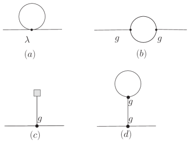
Figure 1: One-loop self energy contributions. $\lambda=\frac{1}{6}\;V^{(IV)}(\Phi_{0})~{},~{}g=\frac{1}{2}\;V^{{}^{\prime\prime\prime}}(\Phi_{0})$. The square box in diagram (c) represents $-C^{3}(\eta)\chi\left[\ddot{\Phi}_{0}+3\,H\;\dot{\Phi}_{0}+V^{{}^{\prime}}_{R}(\Phi_{0})+\mathcal{C}_{2}[\Lambda,H]\;V^{{}^{\prime\prime\prime}}_{R}(\Phi_{0})\right]$. The sum of diagrams (c) and (d) is proportional to the equation of motion (29) and vanishes. Only diagrams (a) and (b) contribute to the self-energy.

$$\Sigma(k,\eta,\eta^{\prime})=\frac{1}{H^{2}_{0}\;\eta^{2}}\left[6\,\lambda\,\left(\mathcal{C}_{2}[\Lambda,H_{0}]+\frac{1}{2}\;\langle[\varphi(\vec{x},\eta)]^{2}\rangle\right)+g^{2}\;\mathcal{C}_{3}[\Lambda,H_{0}]\right]\,\delta(\eta-\eta^{\prime})+\frac{2\,g^{2}}{H^{2}_{0}\,\eta\,\eta^{\prime}}\;\mathcal{K}_{\nu}(k;\eta,\eta^{\prime})\;.$$ (80)

The term proportional to $\delta(\eta-\eta^{\prime})$ is the sum of the contribution from the counterterm $\delta\mathcal{M}^{2}$ and the one loop contribution $(a)$ in fig. 1, while the kernel $\mathcal{K}_{\nu}(k;\eta,\eta^{\prime})$ is determined by the one-loop contribution $(b)$ in fig. 1 and is given byultimonuestro2

$$\mathcal{K}_{\nu}(k;\eta,\eta^{\prime})=2\int\frac{d^{3}q}{(2\pi)^{3}}\;\mathrm{Im}\left[S_{\nu}(q,\eta)S^{*}_{\nu}(q,\eta^{\prime})S_{\nu}(|\vec{q}-\vec{k}|,\eta)S^{*}_{\nu}(|\vec{q}-\vec{k}|,\eta^{\prime})\right]\;,$$ (81)

where the mode functions $S_{\nu}(k,\eta)$ are given by eq. (40). The equation of motion (79) is solved in a perturbative loop expansion as follows

$$X_{\vec{k}}(\eta)=X_{0,\vec{k}}(\eta)+X_{1,\vec{k}}(\eta)+\textmd{higher loop corrections}\;,$$ (82)

where $X_{0,\vec{k}}(\eta)$ is the free field solution, $X_{1,\vec{k}}(\eta)$ is the one-loop correction, etc. This expansion to one loop order leads to the following hierarchy of coupled equations

$$X^{\prime\prime}_{0,\vec{k}}(\eta)+\left[k^{2}-\frac{1}{\eta^{2}}\Big{(}\nu^{2}-\frac{1}{4}\Big{)}\right]X_{0,\vec{k}}(\eta)=0\;,$$ (83)

$$X^{\prime\prime}_{1,\vec{k}}(\eta)+\left[k^{2}-\frac{1}{\eta^{2}}\Big{(}\nu^{2}-\frac{1}{4}\Big{)}\right]X_{1,\vec{k}}(\eta)=\mathcal{R}_{1}(k,\eta)\;,$$ (84)

where the inhomogeneity $\mathcal{R}_{1}(k,\eta)$ due to the interaction of the inflaton is given by

$$\mathcal{R}_{1}(k,\eta)=-\frac{1}{H^{2}_{0}\;\eta^{2}}\left\{\frac{3\,\lambda}{2\,\Delta}\,\left(\frac{H_{0}}{2\,\pi}\right)^{2}+g^{2}\;\mathcal{C}_{3}[\Lambda,H_{0}]\right\}\;X_{0,\vec{k}}(\eta)-\frac{2\,g^{2}}{H^{2}_{0}\;\eta}\int_{\eta_{0}}^{\eta}\frac{d\eta^{\prime}}{\eta^{\prime}}\;\mathcal{K}_{\nu}(k;\eta,\eta^{\prime})\;X_{0,\vec{k}}(\eta^{\prime})\;,$$ (85)

and we have used eqs.(50) and (56). The solution of the inhomogeneous eq.(84) is given by

$$X_{1,\vec{k}}(\eta)=\int_{\eta_{0}}^{0}d\eta^{\prime}\;\mathcal{G}_{\nu}(k;\eta,\eta^{\prime})\;\mathcal{R}_{1}(k,\eta^{\prime})\;.$$ (86)

$\mathcal{G}_{\nu}(k;\eta,\eta^{\prime})$ is the retarded Green’s function obeying

$$\left[\frac{d^{2}}{d\eta^{2}}+k^{2}-\frac{1}{\eta^{2}}\Big{(}\nu^{2}-\frac{1}{4}\Big{)}\right]\mathcal{G}_{\nu}(k;\eta,\eta^{\prime})=\delta(\eta-\eta^{\prime})~{}~{},~{}~{}\mathcal{G}_{\nu}(k;\eta,\eta^{\prime})=0\quad\mathrm{for}\quad\eta^{\prime}>\eta\;.$$ (87)

We are primarily interested in obtaining the superhorizon behavior of the fluctuations ($|k\,\eta|\ll 1$) to obtain the scaling behavior in this limit, therefore we set $k=0$. The kernel $\mathcal{K}_{\nu}(0;\eta,\eta^{\prime})$ was found in referenceultimonuestro2 . To leading order in the slow roll expansion and leading logarithmic order it is given by

$$\mathcal{K}_{\nu}(0;\eta,\eta^{\prime})=\mathcal{K}_{\frac{1}{2}}(0;\eta,\eta^{\prime})+\frac{1}{6\,\pi^{2}}\left[\left(\frac{1}{2\,\Delta}+\frac{2}{3}\right)\left(\frac{\eta^{\prime}}{\eta^{2}}-\frac{\eta}{\eta^{{}^{\prime}2}}\right)-\frac{\eta^{\prime}}{\eta^{2}}\;\ln\frac{\eta^{\prime}}{\eta}+\left(\frac{\eta}{\eta^{{}^{\prime}2}}-\frac{\eta^{\prime}}{\eta^{2}}\right)\,\ln\left(1-\frac{\eta}{\eta^{\prime}}\right)+\frac{1}{\eta^{\prime}}-\frac{1}{\eta}\right]\;,$$ (88)

where

$$\mathcal{K}_{\frac{1}{2}}(0;\eta,\eta^{\prime})=-\frac{1}{8\,\pi^{2}}\;\mathcal{P}\left(\frac{1}{\eta-\eta^{\prime}}\right)=-\frac{1}{8\,\pi^{2}}\;\frac{\eta-\eta^{\prime}}{\left(\eta-\eta^{\prime}\right)^{2}+(\epsilon\;\eta^{\prime})^{2}}\;.$$ (89)

$\epsilon\rightarrow 0$ furnishes a regularization of the principal part prescription in eq. (89) ultimonuestro1 ; ultimonuestro2 . The unperturbed solution and the retarded Green’s function for $k=0$ are the following

$$X_{0,\vec{0}}(\eta) = A\;\eta^{\beta_{+}}+B\;\eta^{\beta_{-}}\quad;\quad\beta_{\pm}\equiv\frac{1}{2}\pm\nu.$$ (90)

$$\mathcal{G}_{\nu}(0,\eta,\eta^{\prime}) = \frac{1}{2\nu}\left[\eta^{\beta_{+}}\;{\eta^{\prime}}^{\beta_{-}}-\eta^{\beta_{-}}\;{\eta^{\prime}}^{\beta_{+}}\right]\Theta(\eta-\eta^{\prime})\;.$$ (91)

where $A$ and $B$ are arbitrary constants. Then, the last term in eq.(85) is

$$\frac{2\,g^{2}}{H^{2}\;\eta}\int_{\eta_{0}}^{\eta}\frac{d\eta^{\prime}}{\eta^{\prime}}\;\mathcal{K}_{\nu}(0;\eta,\eta^{\prime})\;X_{0,0}(\eta^{\prime})=A\;\eta^{\beta_{+}}\;\frac{\alpha_{+}}{\eta^{2}}+B\;\eta^{\beta_{-}}\;\frac{\alpha_{-}}{\eta^{2}}+F[\eta,\eta_{0}]\;,$$ (92)

where $F[\eta,\eta_{0}]$ refers to the contribution of the lower integration limit and does not produce secular terms in $X_{\vec{0}}(\eta)$. The coefficients $\alpha_{\pm}$ are given byultimonuestro2

$$\alpha_{\pm} = \frac{g^{2}}{(2\,\pi\,H_{0})^{2}}\left[\ln\epsilon+\gamma+\psi(\frac{1}{2}\mp\nu)\right]+\frac{g^{2}}{3(\pi\,H_{0})^{2}}\left[\frac{1}{\frac{9}{4}-\nu^{2}}\left(\frac{3}{2\,\Delta}+2+3\,\gamma\right)+\right.$$ (93)

$$\left.+\frac{1}{\nu^{2}-\frac{1}{4}}+\frac{1}{(\nu\pm\frac{3}{2})^{2}}+\frac{\psi(\frac{5}{2}\mp\nu)}{\frac{3}{2}\mp\nu}+\frac{\psi(-\frac{1}{2}\mp\nu)}{\frac{3}{2}\pm\nu}\right]\;,$$

Combining the above results with the first term in eq.(85), requiring that the counterterm $\mathcal{C}_{3}[\Lambda,H_{0}]$ cancels the ultraviolet divergence $\ln\epsilon$ and keeping leading terms of order $1/\Delta^{2}$ in eqs.(93), we find

$$\mathcal{R}_{1}(0,\eta)=A\;\frac{\eta^{\beta_{+}}}{\eta^{2}}\;(2\,\nu\,d^{+})\,+B\;\frac{\eta^{\beta_{-}}}{\eta^{2}}\;(2\,\nu\,d^{-})\,+F[\eta,\eta_{0}]\;,$$ (94)

where the coefficients $d^{\pm}$ of entirely quantum origin (one-loop) are given by

$$d^{+} = -\frac{1}{2\,\nu}\left[\frac{3\,\lambda}{8\,\pi^{2}\,\Delta}+\frac{1}{6\,\pi^{2}}\left(\frac{g}{H_{0}\,\Delta}\right)^{2}\right]$$ (95)

$$d^{-} = -\frac{1}{2\,\nu}\left[\frac{3\,\lambda}{8\,\pi^{2}\,\Delta}+\frac{1}{2\,\pi^{2}}\left(\frac{g}{H_{0}\,\Delta}\right)^{2}\right]\;.$$ (96)

Carrying out the integral in eq. (86) with the retarded Green’s function given by eq. (91) we find the following result for the first order correction,

$$X_{1,0}=A\;\eta^{\beta_{+}}\;d^{+}\ln\left(\frac{\eta}{\eta_{0}}\right)-B\;\eta^{\beta_{-}}\;d^{-}\ln\left(\frac{\eta}{\eta_{0}}\right)+\textmd{non-secular terms}\;,$$ (97)

where the non-secular terms do not grow in the limit $\eta\rightarrow 0$. Up to first order in the loop expansion and leading order in $\Delta$, the solution for superhorizon modes is given by

$$X_{0}(\eta)=A\;\eta^{\beta_{+}}\left[1+d^{+}\ln\left(\frac{\eta}{\eta_{0}}\right)\right]+B\;\eta^{\beta_{-}}\left[1-d^{-}\ln\left(\frac{\eta}{\eta_{0}}\right)\right]+\textmd{non-secular terms}\;.$$ (98)

The resummation of the logarithmic secular terms is performed by implementing the dynamical renormalization group resummation introduced in refs.ultimonuestro1 ; ultimonuestro2 , leading to the following result

$$X_{0}(\eta)=A_{\overline{\eta}}\;\left(\frac{\eta}{\overline{\eta}}\right)^{\beta_{+}+d^{+}}+B_{\overline{\eta}}\;\left(\frac{\eta}{\overline{\eta}}\right)^{\beta_{-}-d^{-}}=\left(\frac{\eta}{\overline{\eta}}\right)^{\Gamma}\left[A_{\overline{\eta}}\;\left(\frac{\eta}{\overline{\eta}}\right)^{\beta_{+}+\gamma}+B_{\overline{\eta}}\;\left(\frac{\eta}{\overline{\eta}}\right)^{\beta_{-}-\gamma}\right]\;,$$ (99)

where $\overline{\eta}$ is a renormalization scale; the amplitudes $A_{\overline{\eta}},\;B_{\overline{\eta}}$ are given at this renormalization scale and obey a renormalization group equation, so that the full solution $X_{0}(\eta)$ is independent of the renormalization scale, as it must be. The exponents are given by

$$\gamma = \frac{1}{2}\left(d^{+}+d^{-}\right)=-\frac{1}{2\,\nu}\left[\frac{3\,\lambda}{8\,\pi^{2}\,\Delta}+\frac{1}{3\,\pi^{2}}\left(\frac{g}{H_{0}\,\Delta}\right)^{2}\right]\;,$$ (100)

$$\Gamma = \frac{1}{2}\left(d^{+}-d^{-}\right)=\frac{1}{12\,\pi^{2}\,\nu}\left(\frac{g}{H_{0}\,\Delta}\right)^{2}\;.$$ (101)

The exponent $\Gamma$ coincides to leading order in slow roll with the result obtained in ref.ultimonuestro2 . Since $\eta=-e^{-H_{0}\,t}/H_{0}$, in comoving time the amplitude of superhorizon fluctuations decays exponentially with the decay rate

$$\Gamma_{\varphi\rightarrow\varphi\varphi}=H_{0}\,\Gamma=\frac{H_{0}}{12\,\pi^{2}\,\nu}\left(\frac{g}{H_{0}\,\Delta}\right)^{2}\;,$$ (102)

where the subscript ${\varphi\rightarrow\varphi\varphi}$ emphasizes that this is the rate of self decay of inflaton fluctuations, a novel phenomenon which is a consequence of the inflationary expansionultimonuestro1 ; ultimonuestro2 .

In ref.ultimonuestro2 no quartic coupling was considered and the exponent $\gamma$ (for $\lambda=0$) was absorbed into a finite redefinition (renormalization) of the mass of the inflaton, or alternatively of $\nu$, since the main goal of ref.ultimonuestro2 was to obtain the decay rate $\Gamma$. While such a redefinition of $\nu$ does not affect the decay rate $\Gamma$, in order to understand the novel scaling dimensions $d^{\pm}$ it must be kept separate because it originates from infrared effects and not from the ultraviolet. The ultraviolet renormalization which is accounted for by the counterterm $\delta\mathcal{M}^{2}$ [eq.(77)], subtracts the cutoff dependent contributions which are independent of the wavevector $k$ (for $k\ll\Lambda$) whereas the contribution $\gamma$ [eq.(100)] arises from the infrared and not from the ultraviolet, as its dependence on $\Delta$ makes manifest. Therefore, the exponent $\gamma$ is a genuine infrared correction to the scaling of the mode functions which cannot be absorbed by the ultraviolet renormalization and emerges unambiguously in the scaling regime ($k\;|\eta|\ll 1$), i. e. physical wavelengths much larger than the Hubble radius. These results are in agreement with ref.ultimonuestro2 for the decay rate $\Gamma$. In addition in the limit $\eta\rightarrow 0^{-}$ the growing mode features a novel scaling dimension $-d^{-}$ namely

$$X_{0}(\eta)\buildrel\eta\to 0\over{=}B_{\overline{\eta}}\;\left(\frac{\eta}{\overline{\eta}}\right)^{\frac{1}{2}-\nu-d^{-}}\;.$$ (103)

This correction to scaling is related to the decay rate $\Gamma$ of superhorizon fluctuations eq.(101). From eqs.(26), (27) and (96), to leading order in slow roll and EFT expansions, $d^{-}$ and the comoving time decay rate $\Gamma_{\varphi\rightarrow\varphi\varphi}$ of superhorizon inflaton fluctuations are given by

$$-d^{-}= \left(\frac{H_{0}}{4\pi\,M_{Pl}}\right)^{\!\!2}\frac{\sigma_{V}\;(\eta_{V}-\epsilon_{V})+6\,\xi^{2}_{V}}{2\,\epsilon_{V}\,(\eta_{V}-\epsilon_{V})^{2}}=\Delta_{\mathcal{R}}^{2}\;\frac{\sigma_{V}\;(\eta_{V}-\epsilon_{V})+6\,\xi^{2}_{V}}{4\,(\eta_{V}-\epsilon_{V})^{2}}\;,$$ (104)

$$\Gamma_{\varphi\rightarrow\varphi\varphi}= \left(\frac{H_{0}}{4\,\pi\;M_{Pl}}\right)^{\!\!2}\frac{H_{0}\;\xi^{2}_{V}}{\epsilon_{V}\,(\eta_{V}-\epsilon_{V})^{2}}=\frac{1}{2}\;\Delta_{\mathcal{R}}^{2}\;\frac{H_{0}\;\xi^{2}_{V}}{(\eta_{V}-\epsilon_{V})^{2}}$$ (105)

where the slow-roll parameters are given by eqs. (11)-(12). Whereas the exponent $\nu=\frac{3}{2}-\Delta=\frac{3}{2}+\epsilon_{V}-\eta_{V}$ is determined by eq.(83) for the free mode functions, the novel scaling exponent $-d^{-}$ is determined by the quantum corrections arising from the interactions. Again eq.(104) highlights an important aspect of the effective field theory approach. The bracket in this expression is formally of first order in slow roll, namely of the same order in slow roll as the departure from scale invariance of the free field mode functions. This is a consequence of the infrared enhancement of the self-energy for $\nu\sim 3/2$ manifest as $\Delta^{-2}=(\eta_{V}-\epsilon_{V})^{-2}$. However, the novel dimension is perturbatively small precisely because of the effective field theory factor $H^{2}_{0}/M^{2}_{Pl}$.

There are two important aspects of the above results that must be compared to our previous studiesultimonuestro1 ; ultimonuestro2 :

• In contrast to the study in ref.ultimonuestro1 ; ultimonuestro2 we have included both the cubic and the quartic interaction vertices. The quartic coupling is of the same order in (EFT) as the square of the cubic coupling but higher order in slow roll [see eqs. (26)-(27)]. However, up to one loop, the diagram with two cubic couplings has two propagators, while the diagram with one quartic coupling has only one propagator. The difference in the number of propagators in these diagrams makes the contribution from the one loop with two cubic couplings of the same order in (EFT) and slow roll as the one loop with one quartic coupling. This is an important difference with our previous study, which a systematic treatment of both the (EFT) and slow-roll approximations as done here, has revealed.

• In our previous studyultimonuestro1 ; ultimonuestro2 the term $\gamma=(d^{+}+d^{-})/2$ in the (DRG) improved solution (99) was absorbed into a finite mass renormalization simply because those studies focused on the decay rate. Here we recognize that the contribution from $\gamma$ is not a mass renormalization but instead enters in the anomalous dimensions of the growing and the decaying modes. This is an important new result, embodied in the final expression (99) which displays both the growing and decaying modes.

VI Inflaton coupling to other light scalars.

So far our analysis only considered the self-interaction of the inflaton. In this section we generalize the previous results to a model which describes the inflaton field coupled to another scalar field $\sigma(x)$ with both trilinear and quartic interactions. The new action is obtained from that in eq.(4) by adding the following terms

$$S_{\sigma}=\int d^{3}x\;dt\;a^{3}(t)\Bigg{\{}\frac{1}{2}\;{\dot{\sigma}^{2}}-\frac{(\nabla\sigma)^{2}}{2a^{2}}-\frac{1}{2}\;m^{2}\;\sigma^{2}-g_{\sigma}\;\phi\;\sigma^{2}-\frac{\lambda_{\sigma}}{2}\;\phi^{2}\;\sigma^{2}\Bigg{\}}$$ (106)

We assume initially zero expectation value for the field $\sigma$ and its time derivative. Thus, $<\sigma>$ vanishes for all times and inflation is still driven by one scalar field.

Upon performing the shift of the inflaton field as in eqn. (2) the effective mass and trilinear coupling are given by

$$m^{2}_{\sigma}(\Phi_{0}) = m^{2}+2\,g_{\sigma}\;\Phi_{0}+\lambda_{\sigma}\;\Phi^{2}_{0}$$ (107)

$$\widetilde{g}_{\sigma}(\Phi_{0}) = g_{\sigma}+\lambda_{\sigma}\;\Phi_{0}.$$ (108)

In what follows we will assume that the sigma field is light in the sense that

$$\frac{m^{2}_{\sigma}(\Phi_{0})}{H^{2}_{0}}\ll 1\;.$$ (109)

Now all the steps in sections III-V generalize to this case. An extra term appears now in the equation of motion of the inflaton (eq.29) at one-loop level,

$$\ddot{\Phi}_{0}(t)+3\,H_{0}\;\dot{\Phi}_{0}(t)+V^{\prime}(\Phi_{0})+g(\Phi_{0})\;\langle[\varphi^{+}(\vec{x},t)]^{2}\rangle+\widetilde{g}_{\sigma}(\Phi_{0})\;\langle[\sigma^{+}(\vec{x},t)]^{2}\rangle=0\;.$$ (110)

We conformally rescale the $\sigma$ field as,

$$\sigma(\vec{x},t)=\frac{\rho(\vec{x},\eta)}{C(\eta)}\;.$$

The spatial Fourier transform of the free field Heisenberg operators $\rho(\vec{x},\eta)$ obey the equation

$$\rho^{{}^{\prime\prime}}_{\vec{k}}(\eta)+\left[k^{2}+m^{2}_{\sigma}(\Phi_{0})\;C^{2}(\eta)-\frac{C^{{}^{\prime\prime}}(\eta)}{C(\eta)}\right]\rho_{\vec{k}}(\eta)=0\,.$$ (111)

Using the slow roll expressions eq.(33), it becomes

$$\rho^{{}^{\prime\prime}}_{\vec{k}}(\eta)+\left[k^{2}-\frac{\bar{\nu}^{2}-\frac{1}{4}}{\eta^{2}}\right]\rho_{\vec{k}}(\eta)=0$$ (112)

where the index $\bar{\nu}$ is given by

$$\bar{\nu}=\frac{3}{2}+\epsilon_{V}-\frac{m^{2}_{\sigma}(\Phi_{0})}{3\,H^{2}_{0}}+\mathcal{O}\left[\epsilon^{2}_{V},\eta^{2}_{V},\epsilon_{V}\eta_{V},\frac{m^{4}_{\sigma}(\Phi_{0})}{\,H^{4}}\right]\,.$$ (113)

The parameter ${\bar{\Delta}}$ which controls the infrared behavior of the $\rho$ fluctuations is given by

$${\bar{\Delta}}\equiv\frac{3}{2}-\bar{\nu}=\frac{m^{2}_{\sigma}(\Phi_{0})}{3\,H^{2}_{0}}-\epsilon_{V}+\mathcal{O}\left[\epsilon^{2}_{V},\eta^{2}_{V},\epsilon_{V}\eta_{V},\frac{m^{4}_{\sigma}(\Phi_{0})}{\,H^{4}_{0}}\right]\;.$$ (114)

Notice that the CMB anisotropy observations indicate that the slow roll parameters are $\lesssim 10^{-2}$ consequently $\Delta$ is also $\lesssim 10^{-2}$. The validity of the slow roll approximation and the condition that the scalar field $\sigma$ be light (109) guarantee that ${\bar{\Delta}}\ll 1$.

The renormalized effective equation of motion (29) becomes

$$\ddot{\Phi}_{0}(t)+3\,H_{0}\,\dot{\Phi}_{0}(t)+V^{{}^{\prime}}_{R}(\Phi_{0})+\left(\frac{H_{0}}{4\,\pi}\right)^{2}\left[\frac{V^{{}^{\prime\prime\prime}}_{R}(\Phi_{0})}{\Delta}+\frac{2\,\widetilde{g}_{\sigma}(\Phi_{0})}{{\bar{\Delta}}}\right]=0\;.$$ (115)

There are now extra diagrams that contribute to the inflaton self-energy $\Sigma(k,\eta,\eta^{\prime})$ [eq.(80)] with the field $\sigma$ in the internal lines. These yield further corrections of order $\widetilde{g}_{\sigma}^{2}$ and $\lambda_{\sigma}$ to the inflaton mode functions $X_{\vec{k}}(\eta)$ through eq.(79). The calculation of these new contributions to $X_{\vec{k}}(\eta)$ is straightforward since the diagram 1 (b) with the field $\sigma$ in the internal loop yields the kernel $\mathcal{K}_{\bar{\nu}}(k;\eta,\eta^{\prime})$ which follows from $\mathcal{K}_{\nu}(k;\eta,\eta^{\prime})$ [eqs.(81 ) and (88)] by simply replacing $\nu$ by $\bar{\nu}$ and accounting properly for the different combinatorial factors in the Feynman diagrams. We obtain the following contributions to the coefficients $d^{\pm}$ from the self-energy correction that features one loop of the $\sigma$ field

$$d^{+}_{\sigma} = -\frac{1}{2\,\nu\,{\bar{\Delta}}}\left\{\frac{\lambda_{\sigma}}{8\,\pi^{2}}+\frac{1}{6\,\pi^{2}\,\Delta}\left[\frac{\widetilde{g}_{\sigma}(\Phi_{0})}{H_{0}}\right]^{2}\right\}$$ (116)

$$d^{-}_{\sigma} = -\frac{1}{2\,\nu\,{\bar{\Delta}}}\left\{\frac{\lambda_{\sigma}}{8\,\pi^{2}}+\frac{1}{2\,\pi^{2}\,\Delta}\left[\frac{\widetilde{g}_{\sigma}(\Phi_{0})}{H_{0}}\right]^{2}\right\}\;.$$ (118)

to leading order for small ${\bar{\Delta}}\ll 1$ and $\Delta\,\ll 1$.

The contribution from the light $\sigma$ field to the inflaton self-energy leads to a further correction to the scaling dimension, given by $-d^{-}_{\sigma}$, and to the decay given by

$$\Gamma^{\sigma}=\frac{1}{2}\left(d^{+}_{\sigma}-d^{-}_{\sigma}\right)=\frac{1}{12\,\pi^{2}\;\nu\Delta\;{\bar{\Delta}}}\left[\frac{\widetilde{g}_{\sigma}(\Phi_{0})}{H_{0}}\right]^{2}$$ (119)

In comoving time the partial rate of superhorizon inflaton fluctuations to decay in a pair of $\sigma$ scalars is given by

$$\Gamma_{\varphi\rightarrow\sigma\sigma}=\frac{H_{0}}{12\,\pi^{2}\;\nu\;\Delta\;{\bar{\Delta}}}\left[\frac{\widetilde{g}_{\sigma}(\Phi_{0})}{H_{0}}\right]^{2}$$ (120)

$\Gamma_{\varphi\rightarrow\sigma\sigma}$ has a similar structure to the inflaton self-coupling decay $\Gamma_{\varphi\rightarrow\varphi\varphi}$ [eq.(102)]. The total rate of superhorizon fluctuations is given by

$$\Gamma_{tot}=\Gamma_{\varphi\rightarrow\varphi\varphi}+\Gamma_{\varphi\rightarrow\sigma\sigma}=\frac{1}{12\,\pi^{2}\;\nu\;\Delta\;H_{0}}\left[\frac{\widetilde{g}_{\sigma}^{2}(\Phi_{0})}{{\bar{\Delta}}}+\frac{g^{2}(\Phi_{0})}{\Delta}\right]\;,$$ (121)

where $\Gamma_{\varphi\rightarrow\varphi\varphi}$ is given by eq. (105).

Depending on the values of the effective couplings and mass $\widetilde{g}_{\sigma}(\Phi_{0})$, $\lambda_{\sigma}$, $m^{2}_{\sigma}(\Phi_{0})$ the value of $d^{\pm}_{\sigma}$ can exceed that of $d^{\pm}$. The value of the couplings of the inflaton to another scalar field must necessarily be small so that there is no large isocurvature perturbation contribution.

VII Conclusions and further questions

Motivated by the current and forthcoming precision CMB data, we study the quantum corrections to the inflationary dynamics arising from inflaton self-interactions. Our approach distinctly treats inflationary dynamics in terms of scalar fields as a renormalized effective field theory (EFT) valid when the scale of inflation is much smaller than the cutoff scale (presumably the Planck scale). We focus on single field slow-roll inflation as a viable model that provides a generic setting for the robust predictions of inflation: almost scale invariant spectrum of gaussian adiabatic perturbations, small ratio of tensor to scalar amplitudes, etc, which is compatible with the WMAP data. The calculations of inflationary parameters within the slow roll expansion are typically based on purely gaussian quantum fluctuations. However, the WMAP data yields a hint of a cubic interaction in the form of the small but non-vanishing ‘jerk’ parameter $\xi_{V}$. Furthermore, self-interactions of fluctuations will necessarily be present if the inflaton potential is non-linear as would be the most natural effective description. In this article we focused in obtaining the lowest order quantum corrections to the following relevant inflationary ingredients:

• The equation of motion for the homogeneous expectation value of the inflaton field.

• The Friedmann equation. The corrections to the Friedmann equation correspond to the quantum contributions in the effective potential since these are interpreted as the expectation value of $T_{00}$ in an homogeneous coherent state. The quantum corrections to the effective potential yield quantum corrections to the slow roll parameters. These are computed to leading order in EFT and slow roll expansions.

• The equations of motion for the quantum fluctuations of the inflaton around its classical value.

The effective field theory approach requires that the ratio of the scale of inflation to the cutoff scale is small, namely $H/M_{Pl}\ll 1$. Slow roll inflation relies on an adiabatic evolution of the scalar field and implies a hierarchy of small dimensionless parameters which are related to derivatives of the scalar potential with respect to the fieldbarrow ; liddle . We combined both approaches to obtain the quantum corrections in the effective field theory to leading order in the (EFT) and slow roll expansions.

Both the one-loop correction to the equation of motion of the inflaton and to the Friedmann equation are determined by the power spectrum of scalar fluctuations. A nearly scale invariant spectrum entails a strong infrared behavior of the loop integral manifest as poles in the small parameter $\Delta=\eta_{V}-\epsilon_{V}+\mathcal{O}(\epsilon^{2}_{V},\eta^{2}_{V},\epsilon_{V}\eta_{V})$, which measures the departure from scale invariance.

This slow roll parameter provides a natural infrared regularization of the loop integrals which allows a controllable and systematic (EFT) and slow roll expansions.

We find that the one-loop effective potential to the leading order in slow-roll and $\Delta$ expansions is given by

$$V_{eff}(\Phi_{0})=V_{R}(\Phi_{0})\left[1+\left(\frac{H_{0}}{4\,\pi\;M_{Pl}}\right)^{2}\frac{\eta_{V}}{\eta_{V}-\epsilon_{V}}+\textmd{higher orders in slow roll}\right]=$$ (122)

(123)

$$=V_{R}(\Phi_{0})\left[1+\frac{\Delta^{2}_{\mathcal{T}}}{32}\frac{n_{s}-1+\frac{3}{8}\;r}{n_{s}-1+\frac{1}{4}\;r}+\textmd{higher orders in slow roll}\right]\;,$$ (124)

where $H_{0}$ and the slow roll parameters are explicit but slowly varying functions of $\Phi_{0}$ given by eqs.(11)-(12). This result is strikingly different from that in Minkowski space-time (see appendix).

¿From this effective potential we obtain the effective slow roll parameters that include quantum corrections. The lowest effective slow roll parameters are given by eqs.(73). A remarkable aspect of the quantum corrections to the effective potential and slow roll parameters (namely the terms of order $H^{2}_{0}/M^{2}_{Pl}$) is that these are of zeroth order in slow roll. This is a consequence of the infrared enhancement from the nearly scale invariant scalar quantum fluctuations.

The equations of motion for the quantum fluctuations of the inflaton around the $\Phi_{0}$ are obtained including the one-loop self-energy corrections. The self-energy features a strong infrared behavior which is regularized by $\Delta$. The perturbative solution of the equations of motion features secular terms that diverge in the long time limit (vanishing conformal time). The dynamical renormalization group programultimonuestro1 ; ultimonuestro2 is implemented to provide a resummation of this perturbative series. The improved solution for superhorizon modes feature two novel aspects: a correction to the scaling exponent and a decay rate. The latter, as anticipated in refs.ultimonuestro1 ; ultimonuestro2 describes the self-decay of inflaton fluctuations. To leading order in the effective field theory and slow-roll expansions we find that the novel scaling dimension and decay rate are given by

$$-d^{-}= \left(\frac{H_{0}}{4\pi\,M_{Pl}}\right)^{\!\!2}\frac{\sigma_{V}\;(\eta_{V}-\epsilon_{V})+6\,\xi^{2}_{V}}{2\,\epsilon_{V}\,(\eta_{V}-\epsilon_{V})^{2}}\;,$$ (125)

$$\Gamma_{\varphi\rightarrow\varphi\varphi}= \left(\frac{H_{0}}{4\pi\,M_{Pl}}\right)^{\!\!2}\frac{H_{0}\;\xi^{2}_{V}}{\epsilon_{V}\,(\eta_{V}-\epsilon_{V})^{2}}.$$ (126)

Both the novel scaling dimension and the decay rate can be expressed in terms of CMB observables inserting eqs.(13) for $\eta_{V},\;\epsilon_{V},\;\xi_{V}$ and $\sigma_{V}$ into eqs.(125).

While the quantum corrections are small, consistently with the effective field theory expansion, they may compete with higher order slow roll corrections in the gaussian approximation. Therefore, in order to gain understanding of the inflationary parameters from high precision data, any high order estimate in the slow roll approximation must be accompanied by an assessment of the quantum corrections arising from the interactions as studied here.

We have generalized these results by studying a model in which the inflaton is coupled to a light scalar field $\sigma$. We have obtained the contribution from a loop of $\sigma$ particles to the effective potential, scaling exponents and the partial rate for the decay of superhorizon fluctuations of the inflaton $\rightarrow\sigma\sigma$.

In this article we have focused on studying the effects of the interaction on the expectation value and the fluctuations of the inflaton field. In order to understand the possible effects of the interaction on curvature perturbations and or gravitational waves, the next stage of the program requires to quantize the perturbations and to compute loop corrections. This will be the focus of forthcoming studies.

Appendix A One loop effective potential and equations of motion in Minkowski space-time: a comparison

In this appendix we establish contact with familiar effective potential both at the level of the equation of motion for the expectation value of the scalar field, as well as the expectation value of $T_{00}$.

In Minkowski space time the spatial Fourier transform of the field operator is given by

$$\varphi_{\vec{k}}(t)=\frac{1}{\sqrt{2\omega_{k}}}\left[a_{\vec{k}}\;e^{-i\omega_{k}\,t}+a^{\dagger}_{-\vec{k}}\;e^{i\omega_{k}\,t}\right]\,,$$ (127)

where the vacuum state is annihilated by $a_{\vec{k}}$ and the frequency is given by

$$\omega_{k}=\sqrt{k^{2}+V^{{}^{\prime\prime}}(\Phi_{0})}\,.$$ (128)

The one-loop contribution to the equation of motion (29) is given by

$$\frac{V^{{}^{\prime\prime\prime}}(\Phi_{0})}{2}\;\langle[\varphi(\vec{x},t)]^{2}\rangle=\frac{V^{{}^{\prime\prime\prime}}(\Phi_{0})}{8\,\pi^{2}}\int^{\Lambda}_{0}\frac{k^{2}}{\omega_{k}}\;dk=\frac{d}{d\Phi_{0}}\left[\frac{1}{4\pi^{2}}\int^{\Lambda}_{0}k^{2}\;\omega_{k}\;dk\right]\,.$$ (129)

The expectation value of $T_{00}=\mathcal{H}$ (Hamiltonian density) in Minkowski space time is given up to one loop by the following expression

$$\langle T_{00}\rangle=\left\langle\frac{1}{2}\;\dot{\phi}^{2}+\frac{1}{2}\;\left(\nabla\phi\right)^{2}+V(\phi)\right\rangle=\frac{1}{2}\;{\dot{\Phi_{0}}}^{2}+V(\Phi_{0})+\left\langle\frac{1}{2}\;\dot{\varphi}^{2}+\frac{1}{2}\;\left({\nabla\varphi}\right)^{2}+\frac{1}{2}\;V^{{}^{\prime\prime}}(\Phi_{0})\;\varphi^{2}+\cdots\right\rangle\;.$$ (130)

The expectation value of the fluctuation contribution is given by

$$\left\langle\frac{1}{2}\;\dot{\varphi}^{2}+\frac{1}{2}\;\left({\nabla\varphi}\right)^{2}+\frac{1}{2}\;V^{{}^{\prime\prime}}(\Phi_{0})\;\varphi^{2}+\cdots\right\rangle=\frac{1}{4\pi^{2}}\int^{\Lambda}_{0}k^{2}\;\omega_{k}\;dk=\frac{\Lambda^{4}}{16\pi^{2}}+\frac{V^{{}^{\prime\prime}}(\Phi_{0})\;\Lambda^{2}}{16\,\pi^{2}}-\frac{[V^{{}^{\prime\prime}}(\Phi_{0})]^{2}}{64\,\pi^{2}}\ln\frac{4\,\Lambda^{2}}{V^{{}^{\prime\prime}}(\Phi_{0})}\;.$$ (131)

Renormalization proceeds as usual by writing the bare Lagrangian in terms of the renormalized potential and counterterms. Choosing the counterterms to cancel the quartic, quadratic and logarithmic ultraviolet divergences, we obtain the familiar renormalized one loop effective potential

$$V_{eff}(\Phi_{0})=V_{R}(\Phi_{0})+\frac{[V^{{}^{\prime\prime}}_{R}(\Phi_{0})]^{2}}{64\,\pi^{2}}\ln\frac{V^{{}^{\prime\prime}}_{R}(\Phi_{0})}{M^{2}}\;,$$ (132)

where $M$ is a renormalization scale. Furthermore from eq. (129) it is clear that the equation of motion for the expectation value is given by

$$\ddot{\Phi}_{0}+V^{{}^{\prime}}_{eff}(\Phi_{0})=0\;.$$ (133)

References

- (1) A. Guth, Phys. Rev. D23, 347 (1981); astro-ph/0404546 (2004).
- (2) A. Albrecht , P. J. Steinhardt, Phys. Rev. Lett. 48,1220 (1982).
- (3) A. D. Linde, Phys. Lett. B108, 389 (1982); Phys. Lett. B129,177 (1983).
- (4) E. W. Kolb , M. S. Turner, The Early Universe Addison Wesley, Redwood City, C.A. 1990.
- (5) P. Coles , F. Lucchin, Cosmology, John Wiley, Chichester, 1995.
- (6) A. R. Liddle , D. H. Lyth, Cosmological Inflation and Large Scale Structure, Cambridge University Press, 2000; Phys. Rept. 231, 1 (1993) and references therein.
- (7) D. H. Lyth , A. Riotto, Phys. Rept. 314, 1 (1999).
- (8) V. F. Mukhanov , G. V. Chibisov, Soviet Phys. JETP Lett. 33, 532 (1981).
- (9) S. W. Hawking, Phys. Lett. B115, 295 (1982).
- (10) A. H. Guth , S. Y. Pi, Phys. Rev. Lett. 49, 1110 (1982).
- (11) A. A. Starobinsky, Phys. Lett. B117, 175 (1982).
- (12) J. M. Bardeen, P. J. Steinhardt , M. S. Turner, Phys. Rev. D28, 679 (1983).
- (13) V. F. Mukhanov, H. A. Feldman , R. H. Brandenberger, Phys. Rept. 215, 203 (1992).
- (14) E. Komatsu et.al. (WMAP collaboration), Astro. Phys. Jour. Supp. 148, 119 (2003).
- (15) D. N. Spergel et.al. (WMAP collaboration), Astro. Phys. Jour. Supp. 148, 175 (2003).
- (16) A. Kogut et.al. (WMAP collaboration) Astro. Phys. Jour. Supp. 148, 161 (2003).
- (17) H. V. Peiris et.al. (WMAP collaboration), Astro. Phys. Jour. Supp. 148, 213 (2003).
- (18) A. R. Liddle, P. Parsons , J. D. Barrow, Phys. Rev. D50, 7222 (1994).
- (19) E. D. Stewart , D. H. Lyth, Phys. Lett. B302, 171 (1993); D. H. Lyth , E. D. Stewart, Phys. Lett.B274, 168 (1992).
- (20) J. Lidsey, A. Liddle, E. Kolb, E. Copeland, T. Barreiro , M. Abney, Rev. of Mod. Phys. 69 373, (1997).
- (21) S. Dodelson, E. D. Stewart, Phys. Rev. D65, 101301 (2002); E. D. Stewart, Phys. Rev. D65, 103508 (2002); E. D. Stewart, J.-O. Gong, Phys. Lett. B510, 1 (2001); J.-O. Gong, E. D. Stewart, Phys. Lett. B538, 213 (2002); J. Choe, J.-O Gong, E. D. Stewart, JCAP 07, 012 (2004).
- (22) D. J. Schwarz, C. A. Terrero-Escalante, A. A. Garcia, Phys. Lett. B517, 243 (2001).
- (23) J. Martin, D. J. Schwarz, Phys. Rev. D67, 083512 (2003).
- (24) R. Casadio, F. Finelli, M. Luzzi, G. Venturi, Phys. Rev. D71, 043517 (2005).
- (25) S. Habib, K. Heitmann, G. Jungman, C. Molina-Paris, Phys. Rev. Lett. 89 281301 (2002); S. Habib, A. Heinen, K. Heitmann, G. Jungman, C. Molina-Paris, Phys. Rev. D70 083507 (2004); S. Habib, K. Heitmann, G. Jungman, Phys. Rev. Lett. 94, 061303 (2005); S. Habib, A. Heinen, K. Heitmann, G. Jungman, Phys. Rev. D71, 043518 (2005).
- (26) T. J. Allen, B. Grinstein , M. B. Wise, Phys. Lett. B197, 66 (1987).
- (27) T. Falk, R. Rangarajan , M. Srednicki, Astrophys. J. 403, L1 (1993); Phys. Rev. D46, 4232 (1992).
- (28) N. Bartolo, E. Komatsu, S. Matarrese , A. Riotto, Phys. Rept. 402, 103 (2004); V. Acquaviva, N. Bartolo, S. Matarrese , A. Riotto, Nucl. Phys. B667, 119 (2003).
- (29) K. Enqvist, A. Mazumdar, M. Postma, Phys. Rev. D67, 121303(R) (2003). S. Tsujikawa, Phys. Rev. D68, 083510 (2003). G. Dvali, A. Gruzinov, M. Zaldarriaga, Phys. Rev. D69, 023505 and 083505 (2004). S. Matarrese, A. Riotto, JCAP 0308 (2003) 007. A. Mazumdar, M. Postma, Phys. Lett. B573, 5 (2003); Erratum-ibid. B585 295 (2004). F. Vernizzi, Phys. Rev. D69, 083526 (2004); R. Allahverdi, Phys. Rev. D70, 043507 (2004).
- (30) D. Boyanovsky, R. Holman , S. Prem Kumar, Phys. Rev. D56, 1958 (1997). S. Naidu , R. Holman, hep-th/0409013.
- (31) D. Boyanovsky , H. J. de Vega Phys. Rev. D70, 063508 (2004).
- (32) D. Boyanovsky, H. J. de Vega , N. G. Sanchez, Phys. Rev. D71, 023509 (2005).
- (33) N. Kaloper, M. Kleban, A. Lawrence and S. Shenker, Phys. Rev. D 66, 123510, (2002); C. P. Burgess, J. M. Cline, R. Holman, JCAP, 0310 (2003) 004. H. J. de Vega, in the Proceedings of the 2002 Chalonge School, Palermo, Italy, edited by N. Sanchez and Y. N. Parijskij, Kluwer, vol. 130, p. 1, astro-ph/0307477.
- (34) D. Cirigliano, H. J. de Vega, N. G. Sanchez, Phys. Rev. D 71, 103518 (2005).
- (35) D. Boyanovsky, H. J. de Vega and R. Holman, Phys. Rev. D49, 2769 (1994). D. Boyanovsky, D. Cormier, H. J. de Vega, R. Holman and S. P. Kumar, Phys. Rev. D57 2166, (1998); D. Boyanovsky, D. Cormier, H. J. de Vega, R. Holman, A. Singh, and M. Srednicki, Phys. Rev. D56, 1939 (1997); D. Boyanovsky, H. J. de Vega, R. Holman and J. F. J. Salgado, Phys. Rev. D54 7570, (1996).
- (36) S. A. Ramsey and B. L. Hu, Phys. Rev. D56. 661, (1997); ibid 678, (1997).
- (37) D. Boyanovsky, D. Cormier, H. J. de Vega, R. Holman and S. P. Kumar, in the Proceedings of the VIth. Erice Chalonge School on Astrofundamental Physics, (Eds. N. Sánchez and A. Zichichi ), Kluwer, 1998.
- (38) P. Anderson, C. Molina-Paris, and E. Mottola, hep-th/0504134.
- (39) R. H. Brandenberger and J. Martin, Mod. Phys. Lett. A16, 999 (2001); C. P. Burgess, J. M. Cline and R. Holman, JCAP 310, 4 (2003); U. H. Danielsson, Phys. Rev. D66, 23511 (2002); L. Sriramkumar and T. Padmanabhan, Phys. Rev. D 71, 103512 (2005).
- (40) A. Vilenkin and L. H. Ford, Phys. Rev. D26, 1231 (1982); T. S. Bunch and P. C. W. Davies, Proc. R. Soc. London A360, 117 (1978).