The rigidly rotating magnetosphere of $\sigma$ Ori E

Abstract

We attempt to characterize the observed variability of the magnetic helium-strong star $\sigma$ Ori E in terms of a recently developed rigidly rotating magnetosphere model. This model predicts the accumulation of circumstellar plasma in two co-rotating clouds, situated in magnetohydrostatic equilibrium at the intersection between magnetic and rotational equators. We find that the model can reproduce well the periodic modulations observed in the star’s light curve, H$\alpha$ emission-line profile, and longitudinal field strength, confirming that it furnishes an essentially correct, quantitative description of the star’s magnetically controlled circumstellar environment.

1. Introduction

As befits its status as the archetype of the helium-strong stars, characterized by elevated photospheric helium abundances, the B2Vpe star $\sigma$ Ori E is the most studied in its class. This is predominantly due to the rich phenomenology of variability manifested by the star, which exhibits modulations in its H$\alpha$ Balmer emission (Walborn, 1974), its helium absorption-line strengths (Pedersen & Thomsen, 1977), its photometric indices (Hesser et al., 1976), its UV continuum flux and resonance-line strengths (Smith & Groote, 2001), its 6 $\rm cm$ radio emission (Leone & Umana, 1993), its linear polarization (Kemp & Herman, 1977), and its longitudinal magnetic field strength (Landstreet & Borra, 1978) — all varying on the same 1.19 $\rm dy$ period identified with the stellar rotation cycle. Based on these extensive observations, an empirical picture has emerged (e.g., Groote & Hunger, 1982; Bolton et al., 1987; Shore, 1993) of the star as an oblique-dipole magnetic rotator, whose field supports two circumstellar clouds situated at the intersections between magnetic and rotational equators.

Following on from previous attempts at devising a theoretical basis for this picture (see, e.g., Nakajima, 1985; Shore & Brown, 1990; Bolton, 1994; Short & Bolton, 1994), Townsend & Owocki (2005, hereafter TO) have recently presented a new theoretical model for the distribution of circumstellar plasma around stars, like $\sigma$ Ori E, that are characterized both by strong magnetic fields (such that the magnetic energy density is very much greater than the plasma energy density) and by significant rotation. The model is built on the notion that plasma, flowing along fixed trajectories prescribed by rigid field lines, experiences an effective potential arising from a combination of the stellar gravitational field and the centrifugal force due to co-rotation. In the vicinity of points where the effective potential undergoes a local minimum, as sampled along a field line, the plasma can settle into a stable configuration of magnetohydrostatic equilibrium.

These concepts, originally advanced by Michel & Sturrock (1974) and Nakajima (1985), are augmented in the TO treatment with a description of the process filling the wells established by local potential minima. In a manner similar to the magnetically confined wind shock (MCWS) model envisaged by Babel & Montmerle (1997a, b), radiatively driven wind streams from opposing footpoints collide at the top of closed magnetic loops, producing strong shocks. The post-shock plasma cools via radiative emission, and then either falls back to the star (see, e.g., ud-Doula & Owocki, 2002, their Fig. 4), or — if the rotation is sufficient — settles into an effective potential well, where it continues to co-rotate in the circumstellar environment and accumulate over time.

A strength of this rigidly rotating magnetosphere (RRM) model is its ability to predict quantitatively, via a semi-analytical approach, the relative circumstellar plasma distribution for arbitrary magnetic field configurations — not just for the simple axisymmetric case of a rotation-axis aligned dipole, to which magnetohydrodynamical simulations have so far been restricted on grounds of computational tractability. In particular, application of the RRM formalism to an oblique-dipole model star leads to a specific prediction (cf. TO) of a density distribution that is sharply peaked into two clouds, situated at the intersections between magnetic and rotational equators. Such a distribution coincides with the observationally inferred picture of $\sigma$ Ori E; thus, it is clear that the RRM model holds promise for understanding both this particular star, and related objects.

This letter presents results from a preliminary investigation into whether the RRM model can simultaneously reproduce the spectroscopic, photometric and magnetic variability exhibited by $\sigma$ Ori E. The following section discusses enhancements we have made to the model since the TO study; Section 3 then confronts the predictions of the model with the observed behaviour of the star. We discuss and summarize our findings in Section 4.

2. Theoretical Developments

Although the RRM treatment presented by TO is quite general, much of their analysis focuses on the specific case of a spherical star, having a dipole magnetic field whose origin coincides with the stellar origin. In the present analysis, we relax both of these restrictions. Specifically, we allow the star to assume a centrifugally distorted figure, by defining its surface not as a sphere but as an isosurface of the effective potential function $\Phi(\mathbf{r})$ (cf. TO, their eqn. 11). This isosurface is set at $\Phi=GM_{\ast}/R_{\rm p}$, where $R_{\rm p}$ denotes the polar radius of the star, and — here and throughout — the other symbols have the same meanings as in TO.

We also allow for the possibility of a decentered dipole field, by introducing a vector $\mathbf{a}$ specifying the displacement of the magnetic origin from the stellar origin. Then, the position vector in the stellar reference frame, $\mathbf{r}$, is related to the magnetic-frame position vector $\tilde{\mathbf{r}}$ via

$$\mathbf{r}=\mathbf{Q}\tilde{\mathbf{r}}+\mathbf{a},$$ (1)

where the orthogonal matrix $\mathbf{Q}$ specifies a rotation by an angle $\beta$ (the dipole obliquity) about the Cartesian $y$ axis. In the TO treatment, $\mathbf{a}$ was set to zero, allowing simple expressions (cf. their eqn. 21) to be obtained relating the spherical polar coordinates in each reference frame. For non-zero $\mathbf{a}$, such expressions do not exist, but the transformation between frames remains well defined.

3. RRM Model

Table 1RRM Model Parameters

$\Omega$	$\varepsilon_{\ast}$	$\beta$	$i$	$\mathbf{a}$
($\Omega_{\rm c}$)		(deg)	(deg)	($R_{\rm p}$)
0.5	$10^{-3}$	55	75	$(-0.041,0.30,-0.029)$

3.1. General Considerations

In Table 1, we summarize the basic parameters for the RRM model of $\sigma$ Ori E. The rotation rate $\Omega=0.5\,\Omega_{\rm c}$ is an estimation based on the star’s 1.19 $\rm dy$ period, while the scale height parameter $\varepsilon_{\ast}$ (cf. TO, eqn. 38) has been assigned a value typical to early-type stars. The choices of the obliquity, $\beta=55\arcdeg$, and observer inclination, $i=75\arcdeg$, have been guided by certain characteristics of the spectroscopic and photometric observations presented below. In particular, the unequal spacing of the light-curve minima of $\sigma$ Ori E, whereby the secondary eclipse follows the primary by $\sim 0.4$ of a rotation phase (see Fig. 1), restricts the possible RRM geometries to those satisfying the approximate relation $\beta+i\approx 130\arcdeg$. A further indication that $i\gtrsim 75\arcdeg$ comes from the fact that, at lower inclinations, the H$\alpha$ variations — which take the form of a double S-wave (see Fig. 2) — would exhibit a central spike when the two curves intersect; but no such spike is observed in the spectroscopy.

The one remaining parameter of the model is the dipole offset vector $\mathbf{a}$. The motivation for assuming a non-zero offset comes from the fact that the primary and secondary eclipses have unequal depths; and that the two curves of the double S-wave are of unequal strength. The offset we select comprises (i) a displacement of the dipole center by $0.3\,R_{\rm p}$ in a direction perpendicular to both magnetic and rotation axes, followed by (ii) a displacement of the dipole center by $-0.05\,R_{\rm p}$ along the magnetic axis. The first displacement produces a density contrast between the two clouds situated at the intersections of the equators, that allows us to achieve a good fit between the model and the observations. The second displacement has little effect on the circumstellar plasma distribution, but its introduction improves the fit to the magnetic field observations. We note that Short & Bolton (1994) also suggested an offset dipole field, in order to explain asymmetries in the field observations.

3.2. Photometry

Figure 1.— Observed (diamonds) and modeled (solid line) Stromgren $u$-band light curves of $\sigma$ Ori E, phased on the star’s 1.19 $\rm dy$ rotation period. The error bars on the observational data are based on conservative estimates of the scatter in the raw data (Hesser et al., 1977, their Fig. 1).

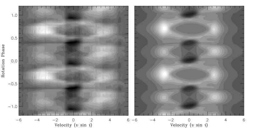
Figure 2.— Observed (left) and modeled (right) time-series grayscales of the circumstellar H$\alpha$ emission of $\sigma$ Ori E, phased on the star’s 1.19 $\rm dy$ rotation period. White indicates a 22% excess (in continuum units) over the background photospheric flux, and black indicates a 12% deficit; the grey levels are scaled linearly between these extremes. The velocity axis is expressed in units of the star’s projected rotation velocity, $v\sin i=160\,\rm km\,s^{-1}$ (Groote & Hunger, 1982).

In Fig. 1, we show the observed Stromgren $u$-band variations of $\sigma$ Ori E, obtained via electronic extraction from Fig. 2 of Hesser et al. (1977). Over these data we plot the synthetic light curve predicted by the RRM model. To calculate this curve, we assume that the photometric variations arise due to absorption of stellar flux by intervening material confined within the co-rotating magnetosphere. Then, the observed $u$-band specific intensity $\mathcal{I}_{u}$, along a given sightline, is evaluated via a simple attenuation expression,

$$\mathcal{I}_{u}=\mathcal{I}_{\ast}\,\rm e^{-\tau_{u}},$$ (2)

where $\mathcal{I}_{\ast}$ is the corresponding intensity at the stellar photosphere, and $\tau_{u}$ is the $u$-band optical depth to the photosphere. The variation of $\mathcal{I}_{\ast}$ across the stellar disk is determined from a combination of the von Zeipel (1924) gravity-darkening law (with the ansatz that the intensity varies in proportion to the bolometric flux) and the Eddington (1926) limb-darkening law. We calculate $\tau_{u}$ from the density distribution predicted by the RRM model, under the assumption that the opacity in the magnetospheric material is spatially constant; this assumption corresponds, for instance, to bound-free absorption processes in a medium having uniform composition and excitation state.

Integrating $\mathcal{I}_{u}$ across the stellar disk, we arrive at the synthetic light curve shown in Fig. 1. Two free parameters enter into this calculation. The normalization of $\mathcal{I}_{\ast}$ is chosen so that the intrinsic (un-obscured) $u$-band brightness of the star is 6.69 $\rm mag$. Likewise, the opacity and density are together scaled to achieve a match with the observed depth of the primary eclipse; this scaling corresponds to a maximal optical depth, over all sightlines and rotation phases, of $\tau_{u}=1.63$.

The agreement between theory and observations is encouraging; the synthetic light curve manages to capture the timing, duration and strength of the eclipses. One obvious mismatch is that the RRM model is unable to reproduce the emission feature at phase $\sim 0.6$, during which the star appears to brighten above its intrinsic level. However, based on the fact that this feature is conspicuously absent from the $u-b$ color variations (cf. Hesser et al., 1977), we believe the feature may arise from some as-yet-unknown photospheric inhomogeneity, rather than from the circumstellar material. Further monitoring is required to test this hypothesis.

3.3. Spectroscopy

In Fig. 2, we plot the circumstellar H$\alpha$ variations exhibited by $\sigma$ Ori E, evaluated by subtracting a phase-dependent synthetic absorption profile from spectroscopic observations of the star (25 echelle spectra, obtained during commissioning of the feros instrument; see Kaufer et al., 1999 and Reiners et al., 2000). The synthetic profiles are calculated using an updated version of the model atmosphere code of Heber (1983), and a photospheric model (see Groote & Hunger, 1997) that takes into account the inhomogeneous helium surface distribution. The resulting synthetic H$\delta$ and H$\gamma$ profiles are in very good agreement with the observations, on account of the absence of significant circumstellar contamination in these lines. Assuming that the synthetic H$\alpha$ profile is also representative of the true (but unknown) photospheric profile, we may interpret the observed-minus-synthetic difference profiles shown in Fig. 2 as an estimated circumstellar component of the total H$\alpha$ flux.

Alongside the observational data, we plot the corresponding predictions of the RRM model. We calculate the monochromatic specific intensity $\mathcal{I}_{\lambda}$ at wavelength $\lambda$, along a given sightline, via formal solution to the equation of radiative transfer,

$$\mathcal{I}_{\lambda}=\mathcal{I}_{\ast}\,\rm e^{-\tau_{\lambda}}+\mathcal{S}\,[1-\rm e^{-\tau_{\lambda}}];$$ (3)

here, $\tau_{\lambda}$ is the monochromatic optical depth, and $\mathcal{S}$ is the source function, assumed to be constant and wavelength independent throughout the circumstellar environment. We model the variation of the photospheric intensity, across the stellar disk, using the same function $\mathcal{I}_{\ast}$ adopted for the $u$-band synthetic photometry (cf. Sec. 3.2); since we are ultimately interested only in the circumstellar component of the H$\alpha$ profile, we do not include any photospheric profile. For sightlines that do not intersect the disk, we set $\mathcal{I}_{\ast}$ to zero.

To derive the optical depth $\tau_{\lambda}$, we assume an opacity proportional to the local plasma density; this choice reflects the fact that H$\alpha$ absorption and emission, via radiative recombination, are density-squared processes. We further assume that the wavelength dependence of the opacity is a Gaussian of full width at half maximum $\Delta\lambda$, centered on the rest-frame wavelength, 6563 Å, of the line. The modeled spectra are calculated by integrating $\mathcal{I}_{\lambda}$ across the stellar disk and surrounding circumstellar region. Three parameters are involved in the synthesis, which we tune by hand to achieve a good fit to the observations. This procedure leads to an intrinsic line width $\Delta\lambda=30\,\rm km\,s^{-1}$, a source function $\mathcal{S}$ set at 0.4 of the maximal photospheric intensity, and an opacity and density scaled such that the maximal optical depth achieved is $\tau_{\lambda}=13.4$.

As with the photometry, there is good agreement between theory and observations. The RRM model correctly reproduces all of the qualitative features of the double S-wave H$\alpha$ variations, including the asymmetry between the red and blue wings, the differing emission strengths at rotation phases $\sim 0.25$ and $\sim 0.75$, and the absorption features at phases $\sim 0.0$ and $\sim 0.4$. The phasing of the synthetic data is based on the photometric fit (cf. Fig. 1); thus, the small phase lag of the model, relative to the observations, can wholly be attributed to the uncertainties in the rotation period (see Reiners et al., 2000) compounded over the two decades separating the photometric and spectroscopic datasets. The contrast between the absorption features seen in the observations (strongest at phase $\sim 0.4$) and in the model (strongest at phase $\sim 0.0$) arises, most likely, due to recent changes in the star’s surface abundance distribution (see Groote, 2003, his Fig. 3) that are not accounted for in our model.

There are, of course, some discrepancies; for instance, the maximal separation of the S-wave curves is somewhat smaller in the model ($\sim 2.75\,v\sin i$) than in the observations ($\sim 3.25\,v\sin i$). Nevertheless, given the many simplifying assumptions incorporated in the RRM model for $\sigma$ Ori E, it is quite striking how well it matches the observed spectroscopic variability of this star.

3.4. Magnetic Field

Figure 3.— Observed (diamonds) and modeled (solid line) longitudinal magnetic field strength of $\sigma$ Ori E, phased on the star’s 1.19 $\rm dy$ rotation period. The open diamonds come from the Landstreet & Borra (1978) dataset, while the filled diamonds are taken from the Bohlender et al. (1987) dataset.

In Fig. 3, we show the time-varying longitudinal magnetic field strength of $\sigma$ Ori E, as measured by Landstreet & Borra (1978) and Bohlender et al. (1987); to maintain consistency with the spectroscopic data, we rephase the field data using the same period and ephemeris adopted by Reiners et al. (2000). Plotted over the observations is the field strength predicted by the RRM model. These synthetic data are calculated via an approach similar to Stibbs (1950): the longitudinal (observer-directed) field is weighted by the local photospheric intensity $\mathcal{I}_{\ast}$ introduced previously, integrated across the stellar disk, and then renormalized by the disk-integrated flux. The field geometry is specified by the parameters given in Table 1, and we choose a field strength such that the flux density is $11\,\rm kG$ at $\pm 1\,R_{\rm p}$ along the magnetic axis. Because the dipole is offset (cf. Sec. 3.1), the actual surface field strengths at the magnetic poles of the star are somewhat different than this nominal value.

Once again, the agreement between theory and observations is encouraging. The reduced chi-squared of the model, 1.79 for 20 degrees of freedom, is rather larger than the value $\chi^{2}/n=1.48$ found by Bohlender et al. (1987) for a sinusoidal fit. However, these authors had the luxury of adjusting the phase of their fit, whereas in the present case the phasing is already constrained by the requirement that the primary light minimum be at phase $0.0$ (cf. Fig. 1). We note that if the two outlier points at phases $\sim 0.05$ and $\sim 0.15$ are discarded, then the correspondence between model and observations improves greatly. Whether these points are indeed erroneous is an matter that should be resolved with further observations.

4. Discussion & Summary

In the preceding sections, we demonstrate how the photometric, spectroscopic and magnetic variability of $\sigma$ Ori E can be reproduced extremely well by a rigidly rotating magnetosphere model. This is persuasive evidence that the RRM paradigm furnishes an essentially correct, quantitative description of the star’s magnetically controlled circumstellar environment.

Future studies can now focus on refining the model and its input parameters, beyond the exploratory treatment that we present here. Furthermore, the analysis can be extended to other observable quantities, such as radio emission, UV line strengths, and polarization. Ultimately, based on our coarse exploration of parameter space, we expect that a fully optimized RRM model will be able to provide strong, independent constraints on the fundamental parameters (e.g., mass, radius) of $\sigma$ Ori E, allowing fresh light to be shed on the historical uncertainty (see Hunger et al., 1989) concerning this exceptional star’s distance and evolutionary status.

References

- Babel & Montmerle (1997a) Babel J., Montmerle T., 1997a, ApJ, 485, 29
- Babel & Montmerle (1997b) Babel J., Montmerle T., 1997b, A&A, 323, 121
- Bohlender et al. (1987) Bohlender D. A., Landstreet J. D., Brown D. N., Thompson I. B., 1987, ApJ, 323, 325
- Bolton (1994) Bolton C. T., 1994, Ap&SS, 221, 95
- Bolton et al. (1987) Bolton C. T., Fullerton A. W., Bohlender D., Landstreet J. D., Gies D. R., 1987, in Slettebak A., Snow T. P., eds, Proc. IAU Colloq. 92: Physics of Be Stars, p. 82
- Eddington (1926) Eddington A. S., 1926, The Internal Constitution of the Stars. Cambridge University Press, Cambridge
- Groote (2003) Groote D., 2003, in Balona L. A., Henrichs H. F., Medupe R., eds, ASP Conf. Ser. 305: Magnetic Fields in O, B and A Stars: Origin and Connection to Pulsation, Rotation and Mass Loss, p. 243
- Groote & Hunger (1982) Groote D., Hunger K., 1982, A&A, 116, 64
- Groote & Hunger (1997) Groote D., Hunger K., 1997, A&A, 319, 250
- Heber (1983) Heber U., 1983, A&A, 118, 39
- Hesser et al. (1977) Hesser J. E., Ugarte P. P., Moreno H., 1977, ApJ, 216, 31
- Hesser et al. (1976) Hesser J. E., Walborn N. R., Ugarte P. P., 1976, Nature, 262, 116
- Hunger et al. (1989) Hunger K., Heber U., Groote D., 1989, A&A, 224, 57
- Kaufer et al. (1999) Kaufer A., Stahl O., Tubbesing S., Norregaard P., Avila G., Francois P., Pasquini L., Pizzella A., 1999, The Messenger, 95, 8
- Kemp & Herman (1977) Kemp J. C., Herman L. C., 1977, ApJ, 218, 770
- Landstreet & Borra (1978) Landstreet J. D., Borra E. F., 1978, ApJ, 224, 5
- Leone & Umana (1993) Leone F., Umana G., 1993, A&A, 268, 667
- Michel & Sturrock (1974) Michel F. C., Sturrock P. A., 1974, Planet. Space Sci., 22, 1501
- Nakajima (1985) Nakajima R., 1985, Ap&SS, 116, 285
- Pedersen & Thomsen (1977) Pedersen H., Thomsen B., 1977, A&AS, 30, 11
- Reiners et al. (2000) Reiners A., Stahl O., Wolf B., Kaufer A., Rivinius T., 2000, A&A, 363, 585
- Shore (1993) Shore S. N., 1993, in Dworetsky M. M., Castelli F., Faraggiana R., eds, Proc. IAU Colloq. 138: Peculiar versus Normal Phenomena in A-type and Related Stars, p. 528
- Shore & Brown (1990) Shore S. N., Brown D. N., 1990, ApJ, 365, 665
- Short & Bolton (1994) Short C. I., Bolton C. T., 1994, in Balona L. A., Henrichs H. F., Contel J. M., eds, Proc. IAU Symp. 162: Pulsation; Rotation; and Mass Loss in Early-Type Stars, p. 171
- Smith & Groote (2001) Smith M. A., Groote D., 2001, A&A, 372, 208
- Stibbs (1950) Stibbs D. W. N., 1950, MNRAS, 110, 395
- Townsend & Owocki (2005) Townsend R. H. D., Owocki S. P., 2005, MNRAS, 357, 251
- ud-Doula & Owocki (2002) ud-Doula A., Owocki S. P., 2002, ApJ, 576, 413
- von Zeipel (1924) von Zeipel H., 1924, MNRAS, 84, 665
- Walborn (1974) Walborn N. R., 1974, ApJ, 191, 95