Laboratory Measurement and Theoretical Modeling of K-shell X-ray Lines from Inner-shell Excited and Ionized Ions of Oxygen

Abstract

We present high resolution laboratory spectra of K-shell X-ray lines from inner-shell excited and ionized ions of oxygen, obtained with a reflection grating spectrometer on the electron beam ion trap (EBIT-I) at the Lawrence Livermore National Laboratory. Only with a multi-ion model including all major atomic collisional and radiative processes, are we able to identify the observed K-shell transitions of oxygen ions from O III to O VI. The wavelengths and associated errors for some of the strongest transitions are given, taking into account both the experimental and modeling uncertainties. The present data should be useful in identifying the absorption features present in astrophysical sources, such as active galactic nuclei and X-ray binaries. They are also useful in providing benchmarks for the testing of theoretical atomic structure calculations.

1 INTRODUCTION

The powerful diffraction grating instruments on board Chandra (Canizares et al., 2000; Brinkman et al., 2000) and XMM-Newton (den Herder et al., 2001) have enabled the observation of K-shell X-ray absorption lines of the ionized plasma surrounding Active Galactic Nuclei (AGNs). Absorption features attributed to various ionization stages of oxgygen ranging from neutral to as high as O VIII have been seen, for example, in NGC 5548, NGC 3783, NGC 4593, and NGC 7469 (Behar et al., 2003; Steenbrugge et al., 2003a, b; Blustin et al., 2003). These new K-shell X-ray absorption measurements complement those in the ultraviolet band (e.g., Arav et al. (2003); Crenshaw et al. (2003)).

One important physical property that can be derived from such measurements is the outflow velocity, which is based on the shift of a given line from its wavelength at rest. Clearly, the accuracy of this procedure depends strongly on the accuracy with which the rest frame wavelength is known (Behar & Kahn, 2002). Calculations offer only limited guidance, as calculations have a rather high uncertainty. A comparison showed that K-shell X-ray line positions of O VI and O V calculated by several authors differ by as much as 60 mÅ and 80 mÅ, respectively (Schmidt et al., 2004). These differences correspond to uncertainties between 800 and 1100 km s^-1, respectively. The spread in the calculated rest frame wavelengths is thus significantly larger than the wavelength shift expected for typical outflow velocities, making most theoretical values nearly useless as rest frame reference standards for a given line. Because of the difficulty of accurately predicting electron-electron correlations, the uncertainty is expected to increase further for calculations of the K-shell X-ray lines of the lower charge states of oxygen. Only laboratory measurements can establish the rest frame wavelengths of a given line and provide an associated uncertainty estimate.

Recently, Schmidt et al. (2004) reported a laboratory measurement of the rest frame wavelengths of the K-shell X-ray resonance lines in O VI and O V. The experimental precision was sufficient to determine flow velocities to within 20 – 40 km s^-1, exceeding the typical measurement accuracy of any current astrophysical X-ray instrument. These measurements were conducted by emission spectroscopy in the interaction of oxygen ions with electrons of sufficient energy to excite the respective K-shell transition. Because the energy needed to excite a K-shell transition is significantly larger than the energy required to ionize all but heliumlike and hydrogenlike oxygen, the measurements had to be performed in a non-equilibrium, ionizing plasma.

Here we report on measurements of K-shell X-ray lines from charge states of oxygen as low as O III. These measurements again utilize emission spectroscopy of oxygen ions excited by high-energy electrons in a non-equilibrium, ionizing plasma. The lines observed under such conditions may be similar to those observed in a photoionized spectrum, where ionization by an electron is replaced by ionization by X rays.

The interpretation of non-equilibrium, ionizing plasmas is difficult. This has recently been shown in various analyses of K-shell iron spectra (Decaux et al., 1997, 2003; Jacobs et al., 1997). Difficulties arise (1) because the wavelengths of the lines are not well known so that the line assignment may be uncertain when clusters of lines are involved and (2) because the excitation processes may be complex, involving an interplay of various processes that are often not fully modeled (if at all), e.g., inner-shell ionization, inner-shell excitation, autoionization, and radiative cascades.

In the simplest case, it is necessary to calculate all excitation, radiative, and autoionization rates affecting a given charge state. Because levels in two neighboring charge states are involved in the formation of spectra due to the presence of autoionization transitions, we denote this model as a “two-ion” model. This model is insufficient to predict the emission in an ionizing plasma where, for example, inner-shell ionization of the neighboring, lower charge state can produce an excited state that in turn contributes to the observed spectrum when undergoing radiative decay. A complex “three-ion” model is typically used to describe the emission from plasmas in which significant ionization and recombination processes take place. Such a model was used, for example, by Doron & Behar (2002) to examine the effect of ionization of Fe XVI and the recombination from Fe XVIII on the Fe XVII X-ray emission. We show that the three-ion model is also insufficient to describe the K-shell oxygen emission observed in our ionizing plasma. In order to describe our observations, we present an “all-ion” model. In this model, the emission of a given ion is coupled to more than just its nearest neighbors. Only this model is found to be able to satisfactorily reproduce the observed oxygen K-shell emission.

The combination of the laboratory data and the all-ion model allows us to identify lines from O III, O IV, O V, and O VI that, to the best of our knowledge, have not yet been measured before. Although many features are likely to be blends of several lines, the features are sufficiently narrow so that we can readily assign wavelengths with small uncertainties. In addition to aiding the identification of lines in absorption spectra, the measured line positions are useful for establishing the quality of wavelength computations and as empirical input for optimizing calculational schemes, such as those carried out recently by Garcia et al. (2004).

2 MEASUREMENT

The measurement was performed at the University of California Lawrence Livermore National Laboratory using the EBIT-I electron beam ion trap. The device has been used for laboratory astrophysics measurements for over a decade (Beiersdorfer, 2003).

The X-ray emission of EBIT-I was detected by a high-resolution grazing incidence spectrometer (Beiersdorfer et al., 2004) with an angle of incidence of 88.5^∘. The spectrometer features a variable line-spaced reflective grating with an average line spacing of 2400 grooves/mm and a radius of curvature of 44.3 m. The spectral image of the ion cloud in the ion trap is nearly flat and permits the use of a two-dimensional charge-coupled device (CCD) as a multichannel detector. The detector is cooled by liquid nitrogen and employs a 27 mm $\times$ 26 mm, thinned, back-illuminated CCD chip with 1340 $\times$ 1300 pixels of 20 $\mu$m $\times$ 20 $\mu$m nominal size; the quantum efficiency is about 45% at 22 Å. In the present setting the detector spans a wavelength interval about 7 Å wide, which is ample to cover the present 21-24 Å range of interest. The resolving power of this setup, drawn from the measured spectra, is about 1100.

Oxygen was introduced to the electron beam ion trap by injection of carbon dioxide. This option provided in situ calibration lines in form of helium-like oxygen (O VII) as well as hydrogen-like carbon (C VI). We observed the resonance, intercombination, and forbidden lines of O VII, denoted $w$, $y$, and $z$, respectively, following the labeling convention introduced by Gabriel (1972). The wavelengths of these lines are well known from the calculations of Drake (1988) and some also from measurements by Engström & Litzén (1995). We also observed the Lyman series in the hydrogen-like spectrum of C VI, $\rm Ly\beta$ through $\rm Ly\varepsilon$, for which Garcia & Mack (1964) provide calculated wavelengths. All these calibration line wavelengths are presumed to be accurate to better than 1 mÅ.

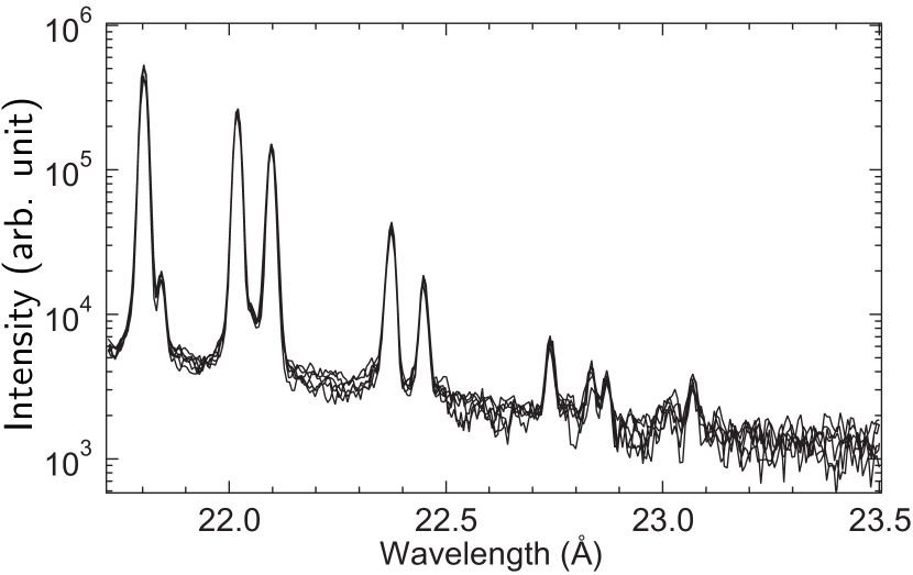
Figure 1: Ten superimposed spectra of oxygen K-shell lines observed in the wavelength range of 21.7 – 23.5 Å. Each spectrum is the result of 120 min observation.

Figure 1 shows features from 21.7–23.5 Å. Ten superimposed spectra, each with 120 min exposure time, show the reproducibility of weak emission features. The black trace in Figure 2 represents the sum of the ten spectra in the wavelength range of 21.4 – 23.2 Å, from 20 h of total observation time. Each of the ten spectra was individually filtered against cosmic ray events, calibrated, and analyzed. The reproducibility of these ten measurements was used to assess statistical and systematic errors.

The measured spectrum in Figure 2 is dominated by the He-like lines $w$, $y$, and $z$. We also readily identify the Li-like line pair $q$ and $r$. These constitute the four strongest lines seen in the spectrum. In addition, the spectrum contains nine features, labeled $A$ – $I$. These satellite lines belong to charge states between O III and O VI. They are situated at the long-wavelength side of the spectrum, and their intensities are considerably weaker than those of the O VII lines. This is partly due to the fact that the upper levels of these transitions have high autoionization rates, and therefore small radiative branching ratios. Another reason lies in the ionization balance; at the electron energies that are needed to excite K-shell lines, the charge state distribution strongly favors O VII, leaving only a small fraction of O VI and a minute abundance of O V and lower charge states (O IV and O III). In fact, the ionization potential of O IV and O III is about 114 eV and 77 eV, respectively, while for technical reasons we used an electron beam energy of 4 keV. We therefore continually supplied neutral oxygen and then detected the different charge states lines (O III through O VI) during the ionizing phase, before the ionization equilibrium was reached. This procedure is similar to that used in earlier measurements of the K-shell emission of low charge state ions of iron (Decaux et al., 1995, 1997).

The wavelengths of all features, $A$ – $I$, are determined relative to the reference lines from O VII and C VI, and are tabulated in Table 1. The uncertainty of the reference lines includes two contributions, one from the errors of their observed positions and the other from their wavelength errors. The uncertainty of reference line positions was added in quadrature to the uncertainty of the line positions of the measured line features. The uncertainty of the reference line wavelengths, which is assumed to be less than 1 mÅ, was added linearly. The overall wavelength uncertainty ranges from 2 to 4 mÅ for line features $C$ – $G$ and $I$, and about 10 – 15 mÅ for $A$, $B$ and $H$.

It is not trivial to unambiguously identify the emission features $A$ – $I$ with specific transitions in various oxygen ions. After examining several theoretical models, we find that only a complex multi-ion model including major collisional and radiative processes is able to account for all line features. In the following we explain the details of these theoretical models, and the most likely identifications of the observed emission lines.

3 THEORETICAL MODELS

The modeling of K-shell emission spectra of L-shell ions under the EBIT-I plasma conditions requires the inclusion of various atomic processes, such as electron collisional excitation, radiative decay, autoionization, and direct electron collisional ionization. With the present beam energy, recombination processes are generally insignificant in populating the excited levels. Because no external radiation field is present in EBIT, we do not include photoionization process in the model. The Flexible Atomic Code (FAC) is used in the present analysis for the basic atomic parameters. FAC is a relativistic configuration interaction atomic code, and uses the distorted-wave approximation to treat electron-ion collision processes (Gu, 2003).

With the given non-equilibrium charge balance for O ions, inner-shell direct electron collisional ionization is expected to be a major process in forming the K-shell lines in addition to the collisional excitation. Moreover, with an electron density of $\approx 10^{12}$ cm^-3 provided by the electron beam current of 120 mA in EBIT-I, many levels in the $1s^{2}2l^{q}$ configurations are significantly populated, and inner-shell excitation as well as ionization from these excited states also play important roles in forming the observed spectrum. To illustrate these effects, we have constructed three theoretical collisional-radiative models with increasing sophistication, which we denote as two-ion, three-ion, and all-ion models. The electron density used in these models, $1.2\times 10^{12}$ cm^-3, is determined by matching the observed O VII line ratio $y/z$, which is density sensitive, to the theoretical result of the all-ion model. In all three models, we only consider the atomic states belonging to the $1s^{2}2l^{q}$, $1s^{2}2l^{q-1}nl$ and $1s2l^{q}nl$ ($2\leq n\leq 4$) configuration complexes for each ion. In the calculation of atomic data, configuration interaction within the same complex is included.

In the two-ion model, we ignore the direct electron collisional ionization processes, and only include collisional excitation followed by radiative cascades and autoionization transitions into the next higher charge state. Therefore, only levels of two neighboring charge states are involved in determining the spectrum of a particular ion. The emission lines from O III – O VII are calculated separately, with the fractional abundance of each charge state adjusted to match the brightest lines observed. The result of this model is shown in the top panel of Figure 2. The relative abundances of O III – O VII ions are 0.36, 0.42, 1.44, 0.77, 1.00, respectively. With this model, it is clear that the intensities of O VII lines $y$ and $z$, and the line features labeled as $D$, $F$, $G$, and $H$ cannot be explained. Feature $C$ is attributed to the O V line $\beta$, and features $E$ and $I$ are attributed to the O IV and O III lines, respectively. Features $A$ and $B$ do not seem to belong to the KLL satellite transitions, and their nature is discussed later in this section. The failure of this model is due to the lack of ionization processes that make contributions to certain lines.

In the three-ion model, we add the next lower charge state to the modeling of the spectrum of a particular ion, and therefore we include the inner-shell electron collisional ionization processes forming K-shell lines in addition to the collisional excitation and autoionization. However, the spectral contributions from individual ions are again treated in separate calculations, with the fractional abundance of each charge state adjusted to match the brightest lines, which are the same as those used in the two-ion model, except that one more ion, O II with a fractional abundance of 0.12 is added to the spectral model of O III. The result of this model is shown in the middle panel of Figure 2. The three-ion model represents a significant improvement over the two-ion model. The O VII lines $y$ and $z$ and the line features D and F are now accounted for satisfactorily. However, feature $H$, which is attributed to the O VI lines $o$ and $p$, is now overpredicted. Lines $o$ and $p$ are mainly produced by the ionization of O V, whose abundance is fixed by matching the $\beta$ line, which is mainly produced by collisional excitation, to the line feature $C$. Therefore the ratio of ($o+p$)/$\beta$ in this model does not depend on the relative abundances of the O VI and O V ions, and is in disagreement with the observed spectrum. Moreover, the observed line feature $G$ cannot be explained satisfactorily in this model. It can be tentatively attributed to the O III lines in its vicinity, which are mainly due to the ionization of O II ions. However, the ionization of O II ions also contributes to the intensity of line feature $I$, and with the chosen abundance of 0.12 for O II, line $I$ is already overpredicted, while the O III lines in the vicinity of $G$ are not nearly strong enough to account for its intensity.

The problems with the three-ion model arise from the fact that only levels in three adjacent charge states are allowed to influence the spectrum of the ion. For example, when calculating the spectrum of O V, only levels in O VI, O V, and O IV enter the model. At very low electron densities, where only the ground state of each charge state is significantly populated, this is a good approximation. At the present electron density, many states in the $1s^{2}2l^{q}$ configurations have large populations relative to the ground state. The ionization of these excited states has an important role in populating the excited states of the next higher charge state, which in turn makes significant contributions to the K-shell lines of even higher charge states. In the example of O V, therefore, all ions having lower charge than O V can indirectly influence the level population of O V through successive ionization. With a three-ion model, such indirect effects are lost. In order to address such far-reaching line formation processes, we have constructed an all-ion model, which includes O I – O VII charge states in a single collisional radiative model. The relative abundances of O I – O VII are adjusted to be 0.01, 0.03, 0.10, 0.15, 0.36, 0.77, and 1.00, respectively, in order to match the brightest lines in the observed spectrum. The small abundances of O I and O II are required by the lack of any significant lines at wavelengths longer than 23.2 Å (see Figure 1). The result of this model is shown in the bottom panel of Figure 2. Unlike the two and three-ion models, this model clearly accounts for all major emission lines in the observed spectrum. An interesting fact is that now line feature $C$ is mainly attributed to the O VI lines $u$ and $v$ instead of O V $\beta$, and feature $G$ is attributed to O V lines, both of which arise due to the step-wise ionization processes from the lower charge states.

The observed spectrum also shows two significant features, $A$ and $B$, on the long wavelength shoulder of the $w$ and $y$ lines. The theoretical models indicate that all $1s^{2}2l-1s2l^{2}$ transitions of O VI, notably, $s$, $t$, $n$, and $m$, are too weak to explain them, and no lines from lower charge states appear in this region. However, the models do give several O VI lines resulting from the $1s^{2}3l^{\prime}-1s2s3l$ ($l^{\prime}=l\pm 1$) transitions in the vicinity of this region, and they have intensities comparable to those observed. These lines are mainly produced by the inner-shell excitation of the O VI ground state, and are enabled only through configuration interaction effects, since the radiative decay involves two-electron transitions. However, due to the difficulties in calculating the radiative and autoionization rates associated with these levels, the confidence in these identifications is somewhat limited.

In Table 1, we list possible line identifications of all significant features from O III – O VI in the observed spectrum. All of these features consist of multiple closely spaced lines, and the theoretical relative intensities of individual lines are given according to the all-ion model. We also compare the measured wavelengths with various theoretical calculations and astrophysical observations, wherever available. In the present calculation, wavelengths are obtained with the configuration interaction (CI) method for all ions, and with a combined CI and second-order many-body perturbation theory method (MBPT) for the KLL transitions of O V and O VI (Gu, 2004). A second-order MBPT calculation is found to have no improvements over the CI method for charge states lower than O V, and therefore the corresponding results are not shown. For O V and O VI, the MBPT correction does seem to improve the theoretical wavelengths significantly.

4 DISCUSSION

Based on the identifications presented in the previous section, we assign measured wavelengths and associated uncertainties to one or two strongest lines in each blended feature, as listed in Table 2. The uncertainties not only reflect the measurement errors, but also take into account the fact that each observed feature contains contributions from weaker lines.

One result of this modeling effort is the recognition that what we had taken to represent line $\beta$ of O V at 22.374(3) Å (Schmidt et al., 2004) is now seen as a contribution to a line blend that is dominated by the O VI satellite lines $u$ and $v$. The line blend has the small wavelength uncertainty determined previously (Schmidt et al., 2004). The individual, unresolved line constituents now have to be assigned larger errors. As we do not see any distortion of the joint line profile from the instrumental profile, line $\beta$ may be assumed to lie within the half width of the line, giving it a line position uncertainty of about 30 mÅ, or ten times more than that of the full line. By comparing the model calculations with the observed spectra, we notice that our new MBPT wavelenghts for other O V and O VI lines agree very well with the measured values. It is therefore reasonable to expect that the MBPT wavelength for line $\beta$ is reliable to within 10 mÅ, and we assign it a wavelength of 22.370(10) Å. This uncertainty of 10 mÅ is about three times larger than previously assumed, but still significantly better than that of ab initio calculations. The uncertainty corresponds to outflow velocity uncertainties of about 130 km s^-1 and is comparable or better than the measurement uncertainty of any current astrophysical measurement.

Line feature $D$ is mainly comprised of six O V transitions with lower and upper configurations of $1s^{2}2s2p$ and $1s2s2p^{2}$, respectively. Of these six lines, the $J=2\to J=2$ transition is the strongest with roughly 40% of the total intensity. All six transitions have theoretical wavelengths within 4 mÅ of each other. Based on the representative wavelength measurement of the complex, we assign an uncertainty of 8 mÅ to the lines in Table 2.

Feature $E$ has two dominant components with 80% of the total intensity. The two transitions have similar theoretical wavelengths. We therefore expect the measured wavelength to be an accurate representation of these two transitions, and we assign a small uncertainty of 5 mÅ to them.

Feature $F$ is almost entirely due to two O IV transitions between $1s^{2}2s2p^{2}$($\frac{5}{2}$,$\frac{3}{2}$) and $1s2s2p^{3}$($\frac{3}{2}$) states. The two transitions have very close theoretical wavelengths, thereofore, we assign the measured wavelength to this blended feature with a small uncertainty.

Feature $G$ is mainly due to the O V transition $1s^{2}2s2p$(2) – $1s2s2p^{2}$(2) with 75% of the total intensity. The remaining blending have the calculated wavelengths very close to the main component. Accordingly, a small uncertainty is assigned to the main component.

Feature $H$ is mainly due to the O VI line pair $o$ and $p$. However, this feature is quite weak and broad. The calculated intensity of $o$ and $p$ does not agree with the observed intensity as well as other features do. It is possible that many weak transitions from other charge states contribute to this feature. We therefore assign a relatively large uncertainty of 20 mÅ to this line pair.

The major component of feature $I$ is the blend of the O III lines $1s^{2}2s^{2}2p^{2}$(1,2) – $1s2s^{2}2p^{3}$(1) with 70% of the total intensity, and having nearly identical theoretical wavelengths. We therefore assign the measured wavelength of this feature as belonging to these two transitions, with a small uncertainty of 6 mÅ.

The wavelengths determined for these transitions in the present work are all significantly better than what is achievable with ab initio calculations, and are better than or at least comparable to the accuracy of the Chandra and XMM-Newton grating instruments. Our data provide reliable reference lines for outflow velocity measurements in the absorption spectroscopy of AGNs and X-ray binaries.

Table 1: Line identifications and wavelength comparisons for K-shell lines of O III – O VI.

Index	$\lambda_{\mbox{exp}}$	Ion	Lower($J$)	Upper($J$)	$f_{ij}$	$\lambda_{\mbox{CI}}$	$\lambda_{\mbox{MBPT}}$	$\lambda_{\mbox{G}}$	$\lambda_{\mbox{VS}}$	$\lambda_{\mbox{C}}$	$\lambda_{\mbox{BK}}$	$\lambda_{\mbox{K}}$	Intensity
$A$	21.672(15)	O VI	$1s^{2}3s$($\frac{1}{2}$)	$1s2p3d$($\frac{3}{2}$)	1.4[-2]	21.600							0.19
		O VI	$1s^{2}3d$($\frac{5}{2}$)	$1s2p3d$($\frac{3}{2}$)	4.5[-3]	21.763							0.18
$B$	21.845(10)	O VI	$1s^{2}3s$($\frac{1}{2}$)	$1s2s3p$($\frac{3}{2}$)	1.6[-2]	21.846							0.58
		O VI	$1s^{2}3s$($\frac{1}{2}$)	$1s2s3p$($\frac{1}{2}$)	7.5[-3]	21.846							0.27
$C$	22.374(3)	O VI	$1s^{2}2s$($\frac{1}{2}$)	$1s2s2p$($\frac{1}{2}$)	2.4[-6]	22.397	22.377	22.37		22.42		22.377(12)	5.49
		O VI	$1s^{2}2s$($\frac{1}{2}$)	$1s2s2p$($\frac{3}{2}$)	1.2[-5]	22.397	22.376		22.373				4.18
		O V	$1s^{2}2s^{2}$(0)	$1s2s^{2}2p$(1)	5.5[-1]	22.363	22.374		22.41	22.33	22.35		1.25
$D$	22.449(3)	O V	$1s^{2}2s2p$(2)	$1s2s2p^{2}$(2)	2.0[-1]	22.465	22.451					22.501(19)	1.65
		O V	$1s^{2}2s2p$(1)	$1s2s2p^{2}$(2)	1.2[-1]	22.464	22.449						0.60
		O V	$1s^{2}2s2p$(2)	$1s2s2p^{2}$(1)	6.6[-2]	22.467	22.453						0.54
		O V	$1s^{2}2s2p$(0)	$1s2s2p^{2}$(1)	2.8[-1]	22.465	22.451						0.46
		O V	$1s^{2}2s2p$(1)	$1s2s2p^{2}$(0)	9.0[-2]	22.466	22.451						0.45
		O V	$1s^{2}2s2p$(1)	$1s2s2p^{2}$(1)	6.3[-2]	22.467	22.452						0.32
$E$	22.741(4)	O IV	$1s^{2}2s^{2}2p$($\frac{3}{2}$)	$1s2s^{2}2p^{2}$($\frac{3}{2}$)	2.0[-1]	22.741			22.75	22.73	22.73	22.740(20)	0.42
		O IV	$1s^{2}2s^{2}2p$($\frac{1}{2}$)	$1s2s^{2}2p^{2}$($\frac{1}{2}$)	1.6[-1]	22.741							0.19
		O IV	$1s^{2}2s^{2}2p$($\frac{3}{2}$)	$1s2s^{2}2p^{2}$($\frac{1}{2}$)	4.0[-2]	22.743							0.09
		O IV	$1s^{2}2s^{2}2p$($\frac{1}{2}$)	$1s2s^{2}2p^{2}$($\frac{3}{2}$)	6.0[-2]	22.739							0.06
$F$	22.836(4)	O IV	$1s^{2}2s2p^{2}$($\frac{5}{2}$)	$1s2s2p^{3}$($\frac{3}{2}$)	1.0[-1]	22.843							0.20
		O IV	$1s^{2}2s2p^{2}$($\frac{3}{2}$)	$1s2s2p^{3}$($\frac{3}{2}$)	1.1[-1]	22.842							0.14
		O IV	$1s^{2}2s2p^{2}$($\frac{1}{2}$)	$1s2s2p^{3}$($\frac{3}{2}$)	1.0[-1]	22.841							0.06
$G$	22.871(4)	O V	$1s^{2}2s2p$(2)	$1s2s2p^{2}$(2)	3.6[-6]	22.882	22.877						0.30
		O V	$1s^{2}2s2p$(2)	$1s2s2p^{2}$(3)	4.2[-6]	22.881	22.875						0.05
		O V	$1s^{2}2s2p$(2)	$1s2s2p^{2}$(1)	3.2[-7]	22.882	22.874						0.04
$H$	23.017(10)	O VI	$1s^{2}2p$($\frac{3}{2}$)	$1s2s^{2}$($\frac{1}{2}$)	3.6[-3]	23.055	23.015	23.00	23.031	23.08			0.06
		O VI	$1s^{2}2p$($\frac{1}{2}$)	$1s2s^{2}$($\frac{1}{2}$)	3.6[-3]	23.053	23.012		23.028				0.03
$I$	23.071(4)	O III	$1s^{2}2s^{2}2p^{2}$(2)	$1s2s^{2}2p^{3}$(1)	8.8[-2]	23.066						23.170(10)	0.13
		O III	$1s^{2}2s^{2}2p^{2}$(1)	$1s2s^{2}2p^{3}$(1)	8.0[-2]	23.065							0.07
		O III	$1s^{2}2s^{2}2p^{2}$(0)	$1s2s^{2}2p^{3}$(1)	1.2[-1]	23.065							0.03
		O III	$1s^{2}2s^{2}2p^{2}$(2)	$1s2s^{2}2p^{3}$(2)	2.0[-1]	23.074							0.03
		O III	$1s^{2}2s^{2}2p^{2}$(2)	$1s2s^{2}2p^{3}$(3)	9.4[-2]	23.086							0.02

Table 2: Best estimate of wavelengths for the strongest transitions of O III – O VI.

Ion	Lower($J$)	Upper($J$)	$\lambda_{\mbox{exp}}$(Å)	Label	Index
O VI	$1s^{2}2s$($\frac{1}{2}$)	$1s2s2p$($\frac{1}{2}$,$\frac{3}{2}$)	22.374(8)	$u$,$v$	$C$
O VI	$1s^{2}2p$($\frac{1}{2}$,$\frac{3}{2}$)	$1s2s^{2}$($\frac{1}{2}$)	23.017(20)	$o$,$p$	$H$
O V	$1s^{2}2s^{2}$(0)	$1s2s^{2}2p$(1)	22.370(10)	$\beta$	$C$
O V	$1s^{2}2s2p$(0,1,2)	$1s2s2p^{2}$(0,1,2)	22.449(8)		$D$
O V	$1s^{2}2s2p$(2)	$1s2s2p^{2}$(2)	22.871(5)		$G$
O IV	$1s^{2}2s^{2}2p$($\frac{1}{2}$,$\frac{3}{2}$)	$1s2s^{2}2p^{2}$($\frac{1}{2}$,$\frac{3}{2}$)	22.741(5)		$E$
O IV	$1s^{2}2s2p^{2}$($\frac{5}{2}$,$\frac{3}{2}$)	$1s2s2p^{3}$($\frac{3}{2}$)	22.836(5)		$F$
O III	$1s^{2}2s^{2}2p^{2}$(1,2)	$1s2s^{2}2p^{3}$(1)	22.071(6)		$I$

Figure 2: Comparison of 2-ion, 3-ion, and all-ion models with the observed spectrum. Black: experiment, red: O VII lines, green: O VI lines, blue: O V lines, magenta: O IV lines, and cyan: O III lines. The theoretical wavelengths in the figure are the configuration interaction results obtained with FAC. The O VI lines have been shifted to the left by 28 mÅ, and the O V lines have been shifted to the left by 10 mÅ. Labels $A$ – $I$ serve to identify the spectral features discussed in the text and listed in Table 1.

References

- Arav et al. (2003) Arav, N., Kaastra, J., Steenbrugge, K., Brinkman, B., Edelson, R., Korista, K. T., & De Kool, M., 2003, ApJ, 590, 174
- Behar & Kahn (2002) Behar, E., & Kahn, S. M., 2002, NASA Laboratory Astrophysics Workshop, held May 1-3 2002 at NASA Ames Research Center, Moffett Field, CA 94035-1000, NASA/CP-2002-21186, 23, also astro-ph/0210280
- Behar et al. (2003) Behar, E., Rasmussen, A. P., Blustin, A. J., Sako, M., Kahn, S. M., Kaastra, J. S., Branduardi-Raymont, G., Steenbrugge, K. C., 2003, ApJ, 598, 232
- Beiersdorfer (2003) Beiersdorfer, P., 2003, ARA&A, 41, 343
- Beiersdorfer et al. (2004) Beiersdorfer, P., Magee, E. W., Träbert, E., Chen, H., Lepson, J. K., Gu, M.-F., & Schmidt, M., 2004, Rev. Sci. Instrum., 75, 3723
- Blustin et al. (2003) Blustin, A. J., Branduardi-Raymont, G., Behar, E., Kaastra, J. S., Kriss, G. A., Page, M. J., Kahn, S. M., Sako, M., & Steenbrugge, K. C., 2003, A&A, 403, 481
- Brinkman et al. (2000) Brinkman, A. C., Gunsing, C. J. T., Kaastra, J. S., van der Meer, R. L. J., Mewe, R., Bräuninger, H., Burkert, W., Burwitz, V., Hartner, G., Predehl, P., Ness, J.-U., Schmitt, J. H. M. M., Drake, J. J., Johnson, O., Juda, M., Kashyap, V., Murray, S., Pease, D., Ratzlaff, P., & Wargelin, B., 2000, ApJ, 530, L111
- Canizares et al. (2000) Canizares, C.R, Huenemoerder, D. P., Davis D. S., Dewey, D., Flanagan, K. A., Houck, J., Markert, T. H., Marshall, H. L., Schattenburg, M. L., Schulz, N. S., Wise, M., Drake, J. J., & Brickhouse, N. S., ApJ, 539, 41
- Chen (1985) Chen, M. H., 1985, Phys. Rev. A, 31, 1449
- Chen (1986) Chen, M. H., 1986, ADNDT, 34, 301
- Chen (1988) Chen, M. H., 1988, ADNDT, 38, 381
- Crenshaw et al. (2003) Crenshaw, D. M., Kraemer, S. B., Gabel, J. R., Kaaastra, J. S., Steenbrugge, K. C., Brinkman, A. C., Dunn, J. P., George, I. M., Liedahl, D. A., Paerels, F. B. S., Turner, T. J., & Yaqoob, T., 2003, ApJ, 594, 116
- Decaux et al. (1995) Decaux, V., Beiersdorfer, P., Osterheld, A., Chen, M., & Kahn, S. M., 1995, ApJ, 443, 464
- Decaux et al. (1997) Decaux, V., Beiersdorfer, P., Kahn, S. M., & Jacobs, V. L., 1997, ApJ, 482, 1076
- Decaux et al. (2003) Decaux, V., Jacobs, V. L., Beiersdorfer, P., Liedahl, D. A., & Kahn, S. M., 2003, Phys. Rev. A, 68, 012509
- den Herder et al. (2001) den Herder, J. W., Brinkman, A. C., Kahn, S. M., Branduardi-Raymond, G., Thomson, K., Aarts, H., Audard, M., Bixler, J. V., den Boggende, A. J., Gottam, J., Decker, T., Dubbeldam, L., Erd, C., Goulooze, H., Güdel, M., Guttridge, P., Hailey, C. J., Al Janabi, K., Kaastra, J. S., de Korte, P. A. J., van Leeuwen, B. J., Mauche, C., McCalden, A. J., Mewe, R., Naber, A., Paerels, F. B., Peterson, J.R., Rasmussen, A. P., Rees, K., Sakelliou, I., Sako, M., Spodek, J., Stern, M., Tamura, T., Tandy, J., de Vries, C. P., Welch, S., & Zehnder, A., 2001, A&A, 365, L7
- Doron & Behar (2002) Doron, R., & Behar, E., 2003, ApJ, 574, 2002
- Drake (1988) Drake, G. W. F., 1988, Can. J. Phys., 66, 586
- Engström & Litzén (1995) Engström, L., & Litzén, U., 1995, J. Phys. B: At. Mol. Opt. Phys., 28, 2565
- Gabriel (1972) Gabriel, A. H., 1972, Mon. Not. R. Astr. Soc., 160, 99
- Garcia & Mack (1964) Garcia, J. D., & Mack, J. E., 1964, J. Opt. Soc. Am., 55, 654
- Garcia et al. (2004) Garcia, J., Mendoza, C., Bautista, M. A., Gorczyca, T. W., Kallman, T. R., & Palmeri, P., 2004, astro-ph/0411374
- Gu (2003) Gu, M. F., 2003, ApJ, 582, 1241
- Gu (2004) Gu, M. F., 2004, ApJS, in press
- Jacobs et al. (1997) Jacobs, V. L., Decaux, V., & Beiersdorfer, P., 1997, J. Quant. Spect. Rad. Transf., 58, 645
- Kaastra et al. (2004) Kaastra, J. S., Raassen, A. J. J., Mewe, R., Arav, N., Behar, E., Costantini, E., Gabel, J. R., Kriss, G. A., Proga, D., Sako, M., & Steenbrugge, K. C., 2004, A&A, 428, 57
- Nicolosi & Tondello (1977) Nicolosi, P., & Tondello, G., 1977, J. Opt. Soc. Am., 67, 1033
- Pradhan et al. (2003) Pradhan, A. K., Chen, G. X., Delahaye, F., Nahar, S. N., & Oelgoetz, J., 2003, Mon. Not. R. Astron. Soc., 341, 1268
- Safronova & Lisina (1979) Safronova, U. I., & Lisina, T. G., 1979, ADNDT, 24, 49
- Schmidt et al. (2004) Schmidt, M., Beiersdorfer, P., Chen, H., Thorn, D. B., Träbert, E., & Behar, E., 2004, ApJ, 604, 562
- Steenbrugge et al. (2003a) Steenbrugge, K. C., Kaastra, J. S., de Vries, C. P., & Edelson, R., 2003, A&A, 402, 477
- Steenbrugge et al. (2003b) Steenbrugge, K. C., Kaastra, J. S., Blustin, A. J., Branduardi-Raymont, G., Sako, M., Behar, E., Kahn, S. M., Paerels, F. B. S., & Walter, R., 2003, A&A, 408, 921
- Vainshtein & Safronova (1978) Vainshtein, L. A., & Safronova, U. I., 1978, ADNDT, 21, 49