Finding SZ clusters in the ACBAR maps

Abstract

We present a new method for component separation from multifrequency maps aimed to extract Sunyaev-Zeldovich (SZ) galaxy clusters from Cosmic Microwave Background (CMB) experiments. This method is best suited to recover non–Gaussian, spatially localized and sparse signals. We apply our method on simulated maps of the ACBAR experiment. We find that this method improves the reconstruction of the integrated $y$ parameter by a factor of three with respect to the Wiener filter case. Moreover, the scatter associated with the reconstruction is reduced by 30 per cent.

1 Introduction

The study of the Cosmic Microwave Background (CMB) has greatly improved our understanding of the Universe in the last decade. The measurement and interpretation of the CMB power spectrum has allowed to determine the most important cosmological parameters with very high accuracy. More experiments, now planned or undeway, will produce higher resolution multi–frequency maps of the sky in the 100–400 GHz frequency range. One of the most important new scientific goals of these experiments is the detection of clusters through their characteristic Sunyaev-Zeldovich (SZ) signature (Sunyaev & Zeldovich 1980). Because the SZ signal is substantially independent of redshift, SZ clusters will be observed at very large distances, quite independently from their mass. Such clusters may be used to infer cosmological information via number counts and power spectrum analysis of SZ maps. Many studies have shown the great potential of these new technique. These estimates, however, typically assume that all clusters above a certain flux are perfectly reconstructed and detected in the CMB maps. In practice, this may not be the case. SZ clusters have radio intensities comparable to other intervening cosmological signals like the CMB and point sources. Despite the different frequency and spatial dependence of these signals, it is not so easy to disentangle them. Moreover, beam smearing and instrumental noise play a role in our ability to adequately reconstruct the observed cluster. These arguments raise the necessity to assess how well a certain technique performs in reconstructing the cluster signal given the experiment specifications. For a given cluster Compton parameter $y$, the reconstructed value may also depend on the cluster location and shape. Therefore, there is an error associated with the reconstruction technique which needs to be assessed and accounted for when it comes to relate cluster’s observables with cosmological models. Moreover, the specific observable to use may depend on the type of experiment in hand. In this paper we address these issues for the ACBAR experiment (see Pierpaoli et al. 2004 for a similar analysis applied to Planck and ACT). Several techniques have been developed for image reconstruction in the multi–component case (Herranz et al. 2002, Stolyarov et al. 2002). In most cases, these techniques are optimal in reconstructing the CMB fluctuation signal, which is Gaussian and well characterized in Fourier space. Clusters of galaxies maps present very different features from CMB ones, in particular: i) clusters are “rare” objects in the map, they don’t fill out the majority of the space; ii) The cluster signal is non–Gaussian on several scales, and in particular on scales associated with the typical core size; iii) Different scales are correlated in Fourier space. Keeping these characteristics in mind, in this paper we develop a method aimed to better reconstruct the SZ galaxy cluster signal from multifrequency maps. Our map reconstruction method is wavelet based and is best suited to reconstruct the specific non–Gaussian signal expected in galaxy clusters maps. In this work we use the simulated cluster maps by Martin White available at: http://pac1.berkeley.edu/tSZ/. These maps are not full hydrodynamical simulations, the gas here has been introduced using the dark matter as a tracer. However for the kind of experiment in hand which would not resolve the cluster structure anyway, this should not present a major problem. The underlying cosmology corresponds to the concordance model. We used ten maps of 10 $\times$ 10 degrees.

Table 1: The characteristics of the ACBAR experiment.

$\nu$ (GHz)	FWHM (arcmin)	noise $(\mu{\rm K}/{\rm beam})$
150	5	6
220	5	10
280	5	12

2 The reconstruction method

2.1 The wavelet decomposition used

We use a two–dimensional overcomplete wavelet representation which is more adequate to the analysis of astrophysical images. The wavelet decomposition of a signal $s$ in our case reads:

$$s=\sum_{q\in N^{2}}\langle s,\phi_{q}\rangle\phi_{q}+\sum_{j=0}^{J}\sum_{m=1}^{M}\sum_{q\in 2^{-j}N^{2}}\langle s,\psi_{j,m,q}\rangle\psi_{j,m,q}$$ (1)

where $\phi_{q}$ are the scaling functions, $\psi_{j,m,q}$ are the wavelets and $\langle,\rangle$ are scalar products. The sum $\sum_{q}\langle s,\phi_{q}\rangle\phi_{q}$ is the projection of $s$ on the coarsest scale, i.e. a low-pass version of $s$. Each scaling coefficient $\langle s,\phi_{q}\rangle$ contains information about the signal $s$ at the coarsest scale and at a specific location in space $q$. For $j$ fixed, the sum $\sum_{m}\sum_{q}\langle s,\psi_{j,m,q}\rangle\psi_{j,m,q}$ is the projection of $s$ on the scale $j$, i.e. a band-pass version of $s$. Each wavelet coefficient $\langle s,\psi_{j,m,q}\rangle$ contains information about the signal $s$ at the specific scale $j$, orientation $m$ and location in space $q$. As usual with wavelet transforms, changing scale is done by dilating, and changing location is done by translating the wavelet: $\psi_{j+1,m,q}(x)=\psi_{j,m,q}(2x)$ and $\psi_{j,m,q}(x)=\psi_{j,m,0}(x-q)$ Hence, scale $j+1$ corresponds to a frequency band that is twice as wide and for which the central frequencies are twice as large as that of scale $j$. On the other hand, in space, the wavelets at scale $j+1$ are better localized than at scale $j$ since they are more narrowly concentrated around their center $q$ (see Fig.1, column 1 and 2).

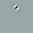
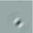
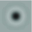
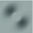
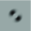
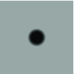
Figure 1: Top row: wavelets in space; Bottom row: wavelets in Fourier plane. Left to right: wavelet at a fine scale $j+1$, centered at location $q_{0}$, oriented along the first diagonal; wavelet at a coarser scale $j$, centered at location $q_{1}$, oriented along the first diagonal; wavelet at the same coarser scale $j$, centered at location $q_{2}$, oriented along the horizontal axis; scaling function, centered at location $q_{2}$.

Unlike the 2-D Daubechies wavelets, the wavelets (and scaling function) we use here are defined in the Fourier plane. This ensures that they are well concentrated in frequency. Moreover, it enables us to introduce orientation by rotating the Fourier transform of the wavelet (see Fig.1, column 2 and 3). If $\tilde{f}$ is the Fourier transform of $f$ and $(r,\theta)$ are polar coordinates, then: $\widetilde{\psi_{j,m,q}}(r,\theta)=\widetilde{\psi_{j,0,q}}(r,\theta-\frac{m\pi}{M})$ The transform is therefore close to rotation invariant and computation is fast via FFT. The Fourier transform of the wavelets and scaling functions read:

$$L(r) = \cos{({\pi\over 2}\log_{2}(r))}\delta_{1<r<2}+\delta_{r<1}\ \ \hbox{ \scriptsize\it low pass}$$ (2)

$$H(r) = \sin{({\pi\over 2}\log_{2}(r))}\delta_{1<r<2}+\delta_{r>2}\ \ \hbox{ \scriptsize\it high pass}$$ (3)

$$G_{M}(\theta) = {(M-1)!\over\sqrt{M[2(M-1)]!}}\left|2\cos\theta\right|^{M-1}\ \ \hbox{ \scriptsize\it oriented}$$ (4)

$$\widetilde{\phi_{0}}(r,\theta) = L(2r,\theta)$$ (5)

$$\widetilde{\psi_{j,m,0}}(r,\theta) = L({r\over{2^{j}}})H({{2r}\over{2^{j}}})G_{M}(\theta-\frac{m\pi}{M})\ \ \ \ \ ^{j\geq 0,}_{0\leq m<M}$$ (6)

The set of all wavelets and scaling functions determines a redundant system (they are linearly dependent), however, the Plancherel equation holds.

2.2 The estimator

Formally, our goal is to estimate several processes (CMB, SZ, point sources) from their contributions in observations at different frequencies. We estimate the processes $\{x(p,\nu_{0})\}_{p}$ from the observations $\{y(\nu)\}_{\nu}$ given that: $y(\nu)=\sum_{p}{f(p,\nu)x(p,\nu_{0})*B(\nu)+N(\nu)}$ where $x(p,\nu_{0})$ is the template of the pth process at a given frequency $\nu_{0}$, $f(p,\nu)$ is the frequency dependence of the pth process, $B(\nu)$ is the beam and $N(\nu)$ is the frequency dependent white noise. Our estimation method will rely on two principles to discriminate the contributions from different processes. The first one is that we know some statistical properties of the processes (e.g. the CMB and noise are Gaussian processes, while the clusters are not). The second one is that some spatial properties of the processes can be captured by modeling the coherence of wavelet coefficients. For example, clusters can be described as spatially localized structures with a high intensity peak. To estimate a particular wavelet coefficient $x_{j,m,q}$, one describes the statistics of a neighborhood of coefficients around it by a Gaussian scale mixture. For example, ${\bf x}_{j,m,q}=(x_{j,m,q},x_{j,m,q+1},x_{j,m,q-1},x_{j-1,m,q})$ is a neighborhood of coefficients around $x_{j,m,q}$. It contains wavelet coefficients at the same scale with close location, and at a close scale with the same location. The Gaussian scale mixture is the model:

$${\bf x}\equiv\sqrt{z}{\bf u}$$ (7)

where ${\bf u}$ is a centered Gaussian vector of the same covariance as ${\bf x}$, the multiplier $z$ is a scalar random variable and the equality holds in distribution. ${\bf u}$ and $z$ are independent and $E\{z\}=1$. The covariance of ${\bf x}$ captures the spatial coherence of the process. The (non-)Gaussianity of the signal is captured by the distribution of the multiplier $z$. To illustrate the idea for the reconstruction process, let us consider the simple case where we observe one process polluted by noise: $y=x+N$ (in wavelet space). ${\bf x}$ is a Gaussian mixture ${\bf x}\equiv\sqrt{z}{\bf u}$, with ${\bf u}$ a Gaussian vector. If $z$ was a constant, $z=z_{0}$, then $E\{{\bf x}|{\bf y},z=z_{0}\}$, the Bayes Least square estimate of ${\bf x}_{j,m,q}$ given the observed vector ${\bf y}_{j,m,q}$ and $z$, would be the Wiener filter:

$$E\{{\bf x}|{\bf y},z=z_{0}\}=z_{0}{\bf C_{x}}(z_{0}{\bf C_{x}}+{\bf C_{N}})^{-1}{\bf y}$$ (8)

where ${\bf C_{v}}$ is the covariance matrix of the vector $v$. However in our model, $z$ is not a constant, so $E\{{\bf x}|{\bf y}\}$, the Bayes Least square estimate of ${\bf x}_{j,m,q}$, is a weighted average of the Wiener filters above:

$$E\{{\bf x}|{\bf y}\}=\int_{0}^{\infty}{p(z=z_{0}|{\bf y})E\{\bf x}|{\bf y},z=z_{0}\}~{}dz_{0}$$ (9)

The weights are determined by the probability of $z$ given the observation ${\bf y}_{j,m,q}$, noted $p(z=z_{0}|{\bf y}_{j,m,q})$, which is computed via Bayes rule:

$$p(z=z_{0}|{\bf y})=\frac{p({\bf y}|z=z_{0})p_{z}(z_{0})}{\int p({\bf y}|z=z^{\prime})p_{z}(z^{\prime})dz^{\prime}}$$ (10)

where $p({\bf y}|z=z^{\prime})$ is a centered Gaussian vector of covariance $z^{\prime}{\bf C_{x}}+{\bf C_{N}}$, and $p_{z}$ is the probability distribution of $z$. Following this procedure, one gets an estimate $E\{{\bf x}_{j,m,q}|{\bf y}_{j,m,q}\}$ for each neighborhood of coefficients ${\bf x}_{j,m,q}$. From this estimated vector, we only keep the estimate of central coefficient $x_{j,m,q}$.

In the case where $p(z)=\delta_{D}(z-0)$, the Gaussian scale mixture described in eq. (7) reduces to a Gaussian process, which is an accurate model for the CMB signal. Other signals, in particular the cluster signal, are typically non–Gaussian. In order to model them, we will need a more elaborate distribution for $z$. In this paper we use a distribution $p(z)$ that we derived from the input SZ maps with the technique described in Pierpaoli et al. (2004). The cluster’s distribution $p(z)$ has a tail for high $z$ values which is caused by the high intensity points in the cluster centers. By using this distribution instead of the delta function (which would correspond to a Gaussian process) we are suggesting to the reconstruction method that in the map there should be more “high intensity” points than in the corresponding Gaussian case with the same variance. In Pierpaoli et al. (2004) we also describe other choices for $p(z)$ and conclude that the final performance in reconstructing the cluster center doesn’t depend on the specific shape of the distribution $p(z)$ provided that $p(z)$ has enough power in the “high–intensity” tail.

3 Results

We applied the method described above to ACBAR simulated maps with realistic beam and noise properties (see table 1). We ignored here the complications in the noise correlation matrix, and assumed instead white noise. We don’t expect this approximation to highly compromise the overall performance. In figures 2 and 3 we show the performances of our method in reconstructing the $y$ parameter of the largest and most intense clusters in the simulations. The reason for such distinction is the following: the method proposed here make use of the spacial covariances of the cluster’s signal. Therefore if the beam size of the experiment is comparable to the typical cluster size (as is the case with ACBAR) clusters with similar intensities but different core size may not be reconstructed equally well, since compact clusters are more likely to be confused with noise. The actual performance in the reconstruction largely depends on the noise level. For this reason we perform the two analysis for “extended” and “intense” clusters separately.

We adopt the following procedure: first we compute the input and output $y$ parameter integrated over a given angle (specified on the $x$ axis); we then fit a line to the input/output values and calculate the average departure of the output values from that line. The figures report the slope of the fitted line (solid lines) and the scatter about it (dashed lines) for the $p(z)$ cluster distribution (blue) and for a delta function corresponding to an hypothetical Gaussian signal (pink).

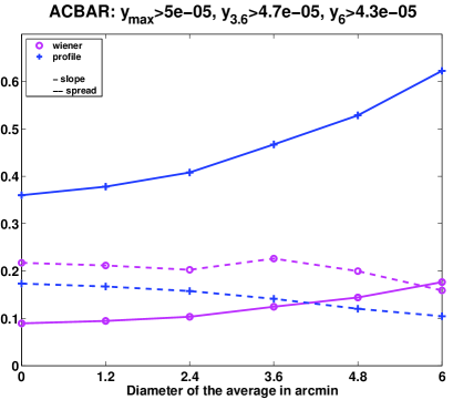
Figure 2: The integrated output $y$ parameter versus the input one for the (12) largest clusters in the simulations. These values are obtained by using the ACBAR specifications. The title indicates the $y$ values of the less intense cluster considered: $y_{max}$, $y_{3.6}$ and $y_{6}$ are the central intensities in the input map with no smoothing (the pixel size of the simulation being 1.17 arcmin) and with a smootihng angle of 3.6 and 6 arcmin respectively.

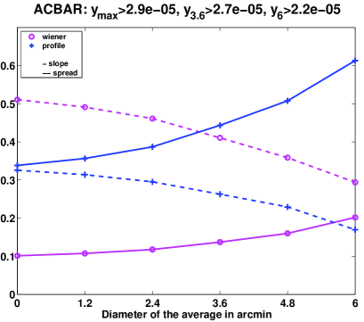
Figure 3: The integrated output $y$ parameter versus the input one for the (34) most intense clusters in the reconstructed maps. The values at the top have the same meaning as in fig. 2. These values are obtained by using the ACBAR specifications.

In these figures we notice that the Wiener filtering (which assumes the delta function for the $p(z)$ distribution) underestimates the high intensity peaks corresponding to massive clusters. The estimator which uses the true $p(z)$ distribution performs on average a factor of three better in reconstructing the central intensity of the clusters, quite independently from the integration angle assumd. The error average departure of the output value from the fitted line is also reduced by about 30 per cent. We conclude that the inclusion of non–Gaussian information greatly improves the reconstruction of clusters SZ signal from observed maps. Performances, however, depends on the specific characteristics of the experiment in hand, as well as on the characteristics of the clusters that we aim to reconstruct (i.e. total intensity and dimensions). In the specific ACBAR case, by comparing figs 2 and 3 we notice that extended clusters are on average slightly better reconstructed and present a significantly lower scatter.

References

- (1) R. A. Sunyaev, I. B. Zeldovich, Microwave background radiation as a probe of the contemporary structure and history of the universe, ARAA 18 (1980) 537–560.
- (2) D. Herranz, J. L. Sanz, M. P. Hobson, R. B. Barreiro, J. M. Diego, E. Martínez-González, A. N. Lasenby, Filtering techniques for the detection of Sunyaev-Zel’dovich clusters in multifrequency maps, MNRAS 336 (2002) 1057–1068.
- Pierpaoli et al. (2004) Pierpaoli E., Anthoine S., Huffenberger K., Daubechies I., 2004, submitted to MNRAS
- (4) V. Stolyarov, M. P. Hobson, M. A. J. Ashdown, A. N. Lasenby, All-sky component separation for the Planck mission, ApJ 336 (2002) 97–111.