An Overview of the Performance of the Chandra X-ray Observatory

Abstract

The Chandra X-ray Observatory is the X-ray component of NASA’s Great Observatory Program which includes the recently launched Spitzer Infrared Telescope, the Hubble Space Telescope (HST) for observations in the visible, and the Compton Gamma-Ray Observatory (CGRO) which, after providing years of useful data has reentered the atmosphere. All these facilities provide, or provided, scientific data to the international astronomical community in response to peer-reviewed proposals for their use. The Chandra X-ray Observatory was the result of the efforts of many academic, commercial, and government organizations primarily in the United States but also in Europe. NASA’s Marshall Space Flight Center (MSFC) manages the Project and provides Project Science; Northrop Grumman Space Technology (NGST – formerly TRW) served as prime contractor responsible for providing the spacecraft, the telescope, and assembling and testing the Observatory; and the Smithsonian Astrophysical Observatory (SAO) provides technical support and is responsible for ground operations including the Chandra X-ray Center (CXC). Telescope and instrument teams at SAO, the Massachusetts Institute of Technology (MIT), the Pennsylvania State University (PSU), the Space Research Institute of the Netherlands (SRON), the Max-Planck Institüt für extraterrestrische Physik (MPE), and the University of Kiel also provide technical support to the Chandra Project. We present here a detailed description of the hardware, its on-orbit performance, and a brief overview of some of the remarkable discoveries that illustrate that performance.

NASA/MSFC, SD50, MSFC AL 35812

SAO, 60 Garden Street, Cambridge MA 02138

MIT, Cambridge MA 02139

SAO, 60 Garden Street, Cambridge MA 02138

MIT, Cambridge MA 02139

SAO, 60 Garden Street, Cambridge MA 02138

MIT, Cambridge MA 02139

MIT, Cambridge MA 02139

SAO, 60 Garden Street, Cambridge MA 02138

1. The Observatory

In 1977, NASA/MSFC and SAO began a study which led to the definition of the then named Advanced X-ray Astrophysics Facility. This study had been initiated as a result of an unsolicited proposal submitted to NASA in 1976 by Prof. R. Giacconi (Harvard University and SAO) and Dr. H. Tananbaum (SAO). Subsequently: the project received the highest recommendation by the National Academy of Sciences Astronomy Survey Committee in the report, ”Astronomy and Astrophysics for the 1980’s”; instruments were selected in 1985; the prime contractor (NGST) was selected in 1988; a demonstration of the ability to build the flight optics was accomplished in 1991; in 1992 the scope of the mission was restructured to reduce cost, including eliminating servicing; the Observatory was named in honor of the Nobel Prize winner Subramanyan Chandrasekhar (Figure 1) in 1998; and the launch occurred the following year. In 2002, Prof. Giacconi (Figure  2) was awarded the Nobel Prize in Physics for his pioneering work in X-ray astronomy.

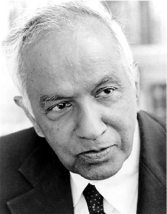
Figure 1.: Professor Subramanyan Chandrasekhar.

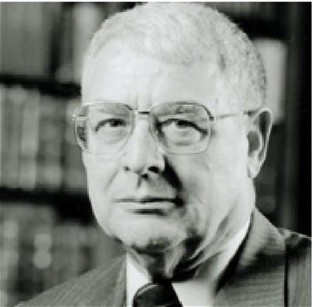
Figure 2.: Professor Riccardo Giacconi.

After two attempts on the evenings of July 19, and July 21 the Observatory was launched on July 23, 1999 using the Space Shuttle Columbia. The Commander was Col. Eileen Collins (Figure 3), the first female commander of a Shuttle flight. The rest of the crew were: Jeffrey Ashby the pilot; and mission specialists Catherine Cady Coleman, Steven Hawley, and Michel Tognini. With a second rocket system, the Inertial Upper Stage (IUS) attached, the Observatory was both the largest and the heaviest payload ever launched by, and deployed from, NASA’s Space Shuttle. Figure 4 shows the IUS mated to the Observatory and both mounted in Columbia’s cargo bay prior to launch.

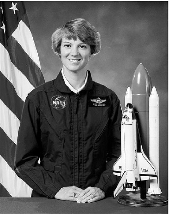
Figure 3.: Col. Eileen Collins.

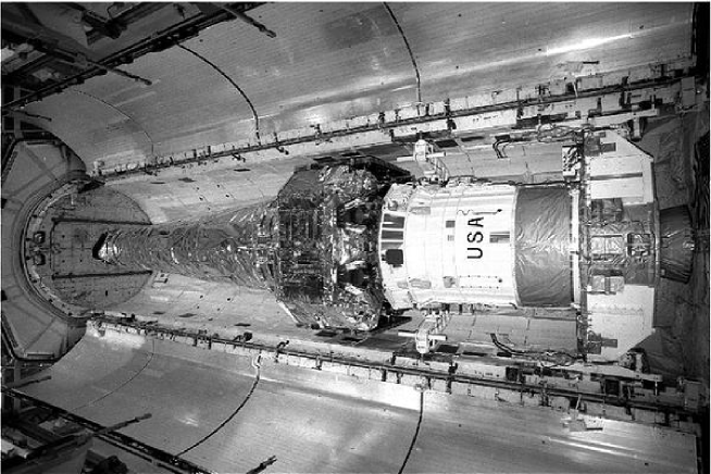
Figure 4.: The Chandra X-ray Observatory with the IUS attached and mounted in the cargo bay of the Space Shuttle Columbia.

After separation from the orbiter, the IUS performed two firings and then separated from the Observatory. The flight system, illustrated in Figure 5, is 13.8-m long by 4.2-m diameter, with a 19.5-m solar-panel wingspan. With extensive use of graphite-epoxy structures, the mass is only 4,800 kg, including almost 1,000 kg of optics. After five firings of an internal propulsion system - the last of which took place 15 days after launch - the Observatory was placed in its highly elliptical orbit. This orbit has a nominal apogee of 140,000 km and a nominal perigee of 10,000 km. The inclination to the equator is 28.5^o. With this orbit, the satellite is above the radiation belts for more than about 75% of the 63.5-hour orbital period. Uninterrupted observations lasting more than 2 days are thus possible. The observing efficiency, which also depends on solar activity, varies from 65% to more than 70%.

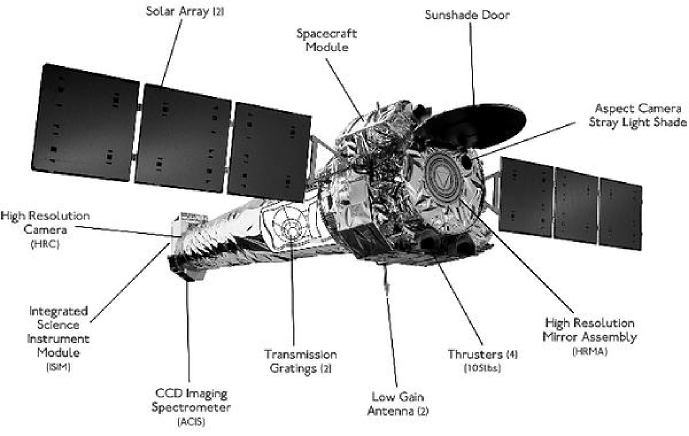
Figure 5.: Artist’s drawing of the Chandra X-ray Observatory with major components labeled.

The spacecraft provides pointing control, power, command and data management, thermal control, and other such services to the scientific payload. Electrical power is obtained from two 3-panel silicon solar arrays that provide over 2000 watts. Three 40-ampere-hour nickel-hydrogen batteries supply power during the rare eclipses. Two low-gain spiral antennas provide spherical communications coverage and the transmission frequency is 2250 MHz. The downlink provides selectable rates from 32 to 1024 kbps for communication with NASA’s Deep Space Network (DSN) of ground stations. Commands are sent at a frequency of 2071.8 MHz and the command rate is 2 kbps. Data are obtained from the instruments at a rate of 24 kbs and are recorded using a solid-state recorder with 1.8 gigabits (16.8 hours) of recording capacity.

Instrument data, together with 8 kbs of spacecraft data, primarily from the aspect camera system, are downloaded to the DSN typically every 8 hours. The ground stations then transmit the information to the Chandra Science Center in Cambridge MA where the operations control center is located. The Observatory is designed to operate autonomously, if necessary, for up to 72 hours and no ground intervention is required to place the Observatory in a safe configuration after a fault is detected. Safe mode has rarely been entered. The spacecraft systems and subsystems have no single-point failure-modes that can threaten the mission.

The principal elements of the payload are the pointing control and aspect system (§ 2.) used to determine where the observatory was pointed, the X-ray telescope (§3.), and the scientific instruments (§ 4., § 5., & § 6.). The specified design life of the mission is 5 years; however, the only perishable (gas for maneuvering) is sized to allow operation for more than 10 years. The orbit will be stable for decades.

2. Pointing Control and Aspect Determination System

The system of sensors and control hardware that is used to point the observatory, maintain the stability, and provide data for determining where the observatory had been pointing is called the Pointing Control and Aspect Determination (PCAD) system. Unlike HST, Chandra pointing requirements are not very stringent because Chandra detectors are essentially single-photon counters and therefore an accurate post-facto history of the spacecraft pointing direction is sufficient to reconstruct the X-ray image.

Here we discuss the PCAD system, how it is used, and the flight performance.

2.1. Physical configuration

The main components of the PCAD system are:

Aspect camera assembly (ACA) – 11.2 cm optical telescope, stray light shade, two CCD  detectors (primary and redundant), and two sets of electronics.

Inertial reference units (IRU) – Two IRUs, each containing two 2-axis gyroscopes.

Fiducial light assemblies (FLA) – LEDs mounted near each X-ray detector which are imaged in the ACA via the Fiducial Transfer System.

Fiducial transfer system (FTS) – directs light from the fiducial lights to the ACA, via a retroreflector collimator (RRC) mounted at the X-ray telescope  center, and a periscope.

Coarse sun sensor (CSS) – Provides all-sky coverage of the sun.

Fine sun sensor (FSS) – Has a 50^o FOV and 0.02^o accuracy.

Earth sensor assembly (ESA) – Conical scanning sensor, used during the orbital insertion phase of the mission.

Reaction wheel assembly (RWA) – 6 momentum wheels which change spacecraft attitude.

Momentum unloading propulsion system (MUPS) – Liquid fuel thrusters which allow RWA momentum unloading.

Reaction control system (RCS) – Thrusters which change spacecraft attitude.

ACA

The aspect camera assembly (Figure 6) includes a sunshade ($\sim$2.5 m long, $\sim$55 cm in diameter), a 11.2 cm, F/9 Ritchey-Chretien optical telescope, and CCD  detector(s). This assembly and its related components are mounted on the side of the X-ray telescope. The camera’s field of view is $1.4^{o}\times 1.4^{o}$ and the sunshade is designed to protect the instrument from the light from the Sun, Earth and Moon, with protection angles of 47^o, 20^o and 6^o, respectively. Only light from the sun can damage the system. Having either the Moon or the Earth in the field-of view only saturates the detector output without incurring damage and therefore only limits the aspects camera’s utility. The Moon (Figure 7) has been viewed with Chandra, in part to study the background signal, and in part to learn about the Moon’s chemical composition.

The aspect camera focal plane detector is a $1024\times 1024$ Scientific Imaging Technologies CCD, with $24\times 24$ micron ($5\times 5$^′′) pixels, covering the spectral band between 4000 and 9000 Å. The CCD  is deliberately placed out of focus (point source FWHM = 9 arcsec) to spread the star images over several pixels in order to increase the accuracy of the centering algorithm, and to reduce variation in the point response function over the field of view. There is a spare CCD, which can be illuminated by rotating a mirror.

The ACA electronics track a small pixel region (either $4\times 4,6\times 6,$ or $8\times 8$ pixels) around the fiducial light and star images. There are a total of eight regions available for tracking. Typically five guide stars and three fiducial lights are tracked. The average background is subtracted on-board, and image centroids are calculated by a weighted-mean algorithm. The image centroids and fluxes are used on-board by the PCAD, and are also telemetered to the ground along with the raw pixel data.

Fiducial lights and Fiducial Transfer System

Surrounding each of the focal-plane detectors is a set of light emitting diodes, or “fiducial lights”, which serve to register the detector focal plane laterally with respect to the ACA boresight. Each fiducial light produces a collimated beam at 635 nm which is imaged onto the ACA via a collimating lens, corner-cube retro-reflector and periscope (Figure 6).

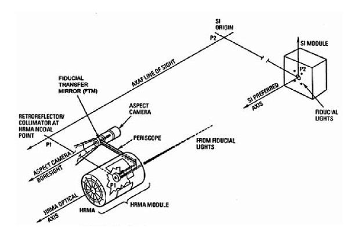
Figure 6.: Schematic diagram of aspect camera assembly and the fiducial transfer system. This illustrates the optical path for imaging the science instrument (SI) fiducial lights onto the ACA. The X-ray telescope is referred to as the High Resolution Mirror Assembly or HRMA.

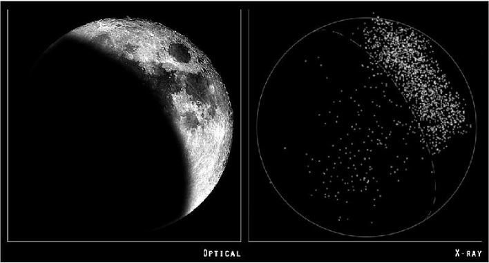
Figure 7.: Optical and X-ray images of the Moon. Optical: Courtesy Robert Gendler; X-ray: NASA/CXC/SAO/J.Drake et al.

Inertial Reference Units

Two Inertial Reference Units (IRU) are located in the front of the observatory on the side of the X-ray telescope. Each IRU contains two gyroscopes, each of which measures an angular rate about 2 axes. This gives a total of eight channels. Data from four of the eight channels can be read out at one time. The gyros are arranged within the IRUs, and the IRUs are oriented, such that the 8 axes are in different directions and no three axes lie in the same plane. The gyros output pulses represent incremental rotation angles. In “high-rate” mode, each pulse nominally represents 0.75^′′, while in “low-rate mode” (used during all normal spacecraft operations) each pulse represents nominally 0.02^′′.

Momentum control

Control of the spacecraft momentum is required both for maneuvers and to maintain stable attitude during observations. Momentum control is primarily accomplished using 6 Teldix RDR-68 reaction wheel units mounted in a pyramidal configuration. During observing, with the spacecraft attitude constant apart from dither (introduced to avoid having the flux from a point source illuminate only a single focal plane detector pixel), external torques on the spacecraft (e.g. gravity gradient, magnetic) will cause a buildup of momentum in the reaction wheel assembly. Momentum is shed from the reaction wheels by firing small thrusters in the MUPS and simultaneously spinning down the reaction wheels.

2.2. Operating principles

The aspect system serves two primary purposes: on-board spacecraft pointing control and aspect determination, and post-facto ground aspect determination, used in X-ray image reconstruction and celestial location.

The PCAD  system has 9 operational modes (6 normal and 3 safe modes) which use different combinations of sensor inputs and control mechanisms to control the spacecraft and ensure its safety. In the normal pointing mode, the PCAD  system uses sensor data from the ACA and IRUs, and control torques from the RWAs, to keep the X-ray target well within $\sim$30^′′ of the desired location. This is done by smoothing (filtering) the data that have been taken during the preceding time intervals using aspect camera star centroids (typically 5) and angular displacement data from two of the 2-axis gyroscopes. On short time scales ($\sim$seconds) the spacecraft motion solution is dominated by the gyroscope data, while on longer timescales it is the star centroids that dominate.

The post-facto aspect determination is done on the ground and uses more sophisticated processing and better calibration data to produce a more accurate solution. The key improvements over the in-flight aspect come from better image centroiding and smoothing all available data over the observation period – as opposed to only a limited set of historical data. In addition, the aspect solution also accounts for the position of the focal-plane instrument as determined by the images of the fiducial lights.

2.3. Performance

The important PCAD  system performance parameters and a comparison to the original requirements are shown in Table 1. In each case the actual performance far exceeds the requirements.

Celestial location accuracy measures the absolute accuracy of Chandra X-ray source locations. Based on observations of 225 point sources detected within 2^′ of the boresight and having accurately known coordinates, the 90% source location error circle has a radius of 0.64^′′ (Figure 8). Fewer than 1% of sources are outside a 1^′′ radius.

Figure 8.: Cumulative histogram of celestial accuracy for Chandra X-ray source locations. Radial offset is the distance in arcsec between the optical coordinate, typically from the Tycho-2 catalog (see http://www.astro.ku.dk/ẽrik/Tycho-2/), and the Chandra position.

The image reconstruction performance measures the effective blurring of the X-ray point spread function (PSF) due to aspect reconstruction. A direct measure of this parameter can be made by determining the time-dependent jitter in the centroid coordinates of a fixed celestial source. Any error in the aspect solution will appear as an apparent wobble in the source location. Unfortunately this method has limitations. When an Advanced CCD Imaging Spectrometer (ACIS - § 4.) detector is at the focus, data are count-rate limited and we find only an upper limit: aspect reconstruction effectively convolves the X-ray telescope PSF with a Gaussian having FWHM of less than 0.25^′′. With an High Resolution Camera (HRC - § 4.) detector at the focus, observations can produce acceptably high count rates, but the current HRC photon positions have systematic errors due to uncertainties in the HRC calibration. These errors exactly mimic the expected dither-dependent signature of aspect reconstruction errors, so no such analysis with HRC data has been done. An indirect method of estimating aspect reconstruction blurring is to use the aspect solution to de-dither the ACA star images and measure the residual jitter. We have done this for 350 observations and find that 99% of the time the effective blurring is less than 0.20^′′ (FWHM).

Absolute celestial pointing is defined as the accuracy with which the Chandra line of sight (the line connecting the nominal aimpoint on the detector and the X-ray telescope node) can be pointed toward a particular target location on the sky, and is about 3^′′ in radius. This result is based on the spread of apparent fiducial light locations for $\sim 1000$ observations in the year 2002. It should be noted that the 3^′′ value represents the repeatability of absolute pointing on timescales of less than approximately one year. During the first 4 years of the mission, there was an exponentially decaying drift in the nominal aimpoint of about 10^′′, most likely due to the expected long-term relaxation in spacecraft structures.

The PCAD  10-second pointing stability performance is measured by calculating the RMS attitude control error (1-axis) over successive 10 second intervals. The attitude control error is simply the difference between the ideal (commanded) dither pattern and the actual measured attitude. Flight data show that after removing known systematic effects, 95% of the RMS error measurements are less than 0.04^′′ (pitch) and 0.03^′′ (yaw).

Table 1.: Aspect System Requirements and Performance

Description	Requirement	Actual
Celestial location	1.0′′  (RMS radius)	0.6′′
Image reconstruction	0.5′′  (RMS diameter)	0.3′′
Absolute celestial pointing	30.0′′  (99.0%, radial)	3.0′′
PCAD  10 sec pointing stability	0.25′′ (RMS, 1-axis)	0.043′′ (pitch)
		0.030′′ (yaw)

2.4. ACA CCD Dark Current

Damage caused by exposure to cosmic rays produces an increase in both the mean CCD  dark current and the non-Gaussian tail of “warm” (damaged) pixels in the aspect camera CCD. Figure 9 shows the distribution of dark current shortly after launch (gray) and in 2003-Apr (black). The background non-uniformity caused by warm pixels (dark current $>100$ e^-/sec) is the main contributor to the star centroiding error, though the effect is substantially reduced by code within the aspect data analysis software which detects and removes most warm pixels from further consideration.

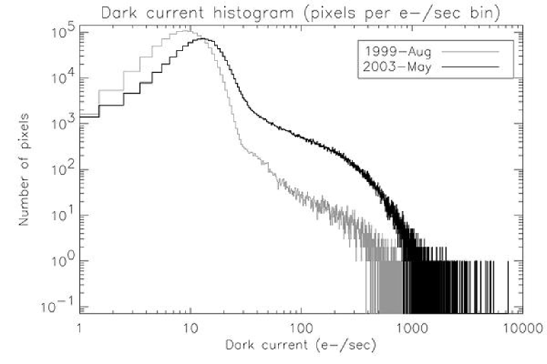
Figure 9.: Differential histogram of dark current distribution for the ACA CCD in 1999-Aug (gray) and 2003-Apr (black)

Prior to May-2003, the number of warm pixels was increasing at a rate of 2% of the CCD pixels per year. At that time the operating temperature of the CCD was lowered from -10 C to -15 C which had the effect of decreasing the dark current by a factor of almost 2, and thereby reducing the number of warm pixels by 40%. At the current operating temperature one expects no further degradation of X-ray image quality (due to aspect) even after 15 years on orbit.

3. The X-ray Optics

The heart of the Observatory is the X-ray telescope made of four concentric, precision-figured, superpolished Wolter-1 telescopes, similar in design to those used for both the Einstein and Rosat observatories, but of much higher quality, larger diameter, and longer focal length. Hughes Danbury Optical Systems (HDOS, Danbury, Connecticut) precision figured and superpolished the 4-mirror-pair grazing-incidence X-ray optics out of Zerodur blanks from Schott Glaswerke (Mainz, Germany). Zerodur, a glassy ceramic, was chosen for its high thermal stability. Optical Coating Laboratory Incorporated (OCLI, Santa Rosa, California) coated the optics with iridium, chosen for high x-ray reflectivity and chemical stability. The Eastman Kodak Company (Rochester, New York) aligned and assembled the mirrors into the 10-m focal length telescope assembly. Recently (2002), the Chandra Telescope Scientist, Leon Van Speybroeck, received the Rossi Prize of the High Energy Astrophysics Division of the American Astronomical Society in recognition of his contributions to X-ray astronomy especially for his role in the design and development of the Chandra optics.

The photograph shown in Figure 10 was taken during the telescope assembly and alignment process. The telescope is inverted in Figure 10 and one sees one of the hyperboloids being lowered into place. Each individual element is 83.3 cm long and polished to better than a few angstroms root-mean-square (RMS) microrougness. The inner surfaces of revolution are coated with 600 angstroms of iridium. The Set of 8 mirrors weighs 956 kg. The focal Length is 10 meters, the outer diameter is 1.2 meters, the field of view is 1^o (FWHM) in diameter, and the clear aperture is 1136 cm².

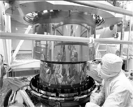
Figure 10.: Photograph of the X-ray telescope during assembly and alignment. Here one of the hyperboloids is being lowered into place prior to alignment and bonding.

3.1. Point Spread Function

The telescope’s point spread function, as measured during ground calibration, had a full width at half-maximum less than 0.5 arcsec and a half-power diameter less than 1 arcsec. The pre-launch prediction for the on-orbit encircled-energy fraction was that a 1-arcsec-diameter circle would enclose at least half the flux from a point source. A relatively mild dependence on energy, resulting from diffractive scattering by surface microroughness, attests to the better than 3-angstroms-rms surface roughness measured with optical metrology during fabrication and confirmed by the ground X-ray testing. The ground measurements were performed at the X-ray Calibration Facility (XRCF) at NASA’s Marshall Space Flight Center (Figure 11). The effects of gravity, the finite source distance, and the size of the various X-ray sources used to calibrate the observatory were unique to the ground calibration and had to be accounted for to determine the on-orbit performance. On-orbit the performance also includes the spatial resolution of the detectors and uncertainties in the aspect solution, although as discussed in § 2.3. this latter is very small. The on-orbit performance met expectations as illustrated in Figure 12.

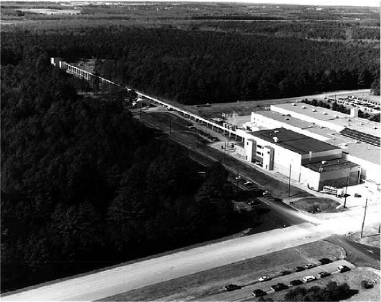
Figure 11.: Aerial view of the X-ray Calibration Facility at NASA’s Marshall Space Flight Center. The large building to the right houses a thermal-vacuum chamber. A 525-m evacuated tube connects the chamber to various X-ray sources located in the building to the far left.

Figure 12.: The predicted and observed fractional encircled energy as a function of radius for an on-axis point source observed with the HRC-I at the focus of the telescope. The calculations at two energies, 0.277 keV and 6.40 keV, include an aspect solution with a rms uncertainty of 0.2 arcsec. Flight data from an observation of AR Lac are also shown.

4. The Focal Plane Cameras

4.1. ACIS

The Pennsylvania State University (PSU, University Park, Pennsylvania) and MIT designed and fabricated the ACIS with CCDs produced by MIT Lincoln Laboratory (Lexington, Massachusetts). Some subsystems and systems integration were provided by Lockheed-Martin Astronautics (Littleton, Colorado). Made of a 2-by-2 array of large-format, front-illuminated (FI), 2.5-cm-square, CCDs, ACIS-I provides high-resolution spectrometric imaging over a 17-arcmin-square field of view. ACIS-S, a 6-by-1 array of 4 FI CCDs and two back-illuminated (BI) CCDs mounted along the transmission grating (§ 6.) dispersion direction, serves both as the primary read-out detector for the High Energy Transmission Grating (HETG - § 6.2.), and, using the one BI CCD which can be placed at the aimpoint of the telescope, also provides high-resolution spectrometric imaging extending to lower energies but over a smaller (8-arcmin-square) field than ACIS-I. Both ACIS detectors are covered with aluminized-polyimide filters, designed to block visible light. A picture of the instrument is shown in Figure 13 and a block diagram with additional details is shown in Figure 14 Many of the characteristics of the ACIS instrument are summarized in Table 2.

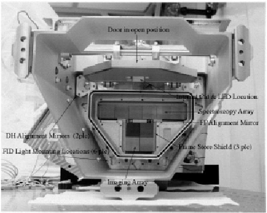
Figure 13.: Photograph of the focal plane of ACIS, prior to installation of the optical blocking filters. The ACIS-I is at the bottom; the ACIS-S (the readout for the HETG), at the top.

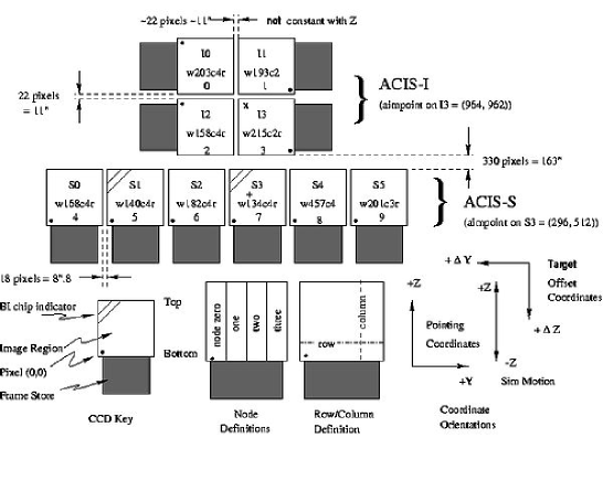
Figure 14.: A schematic of the ACIS focal plane. The view is along the optical axis, from the source toward the detectors. The nominal aimpoints are indicated by the ‘+’ on S3 and the ‘x’ on I3. The numerous ways to refer to a particular CCD are also shown: chip letter+number, chip serial number, and ACIS chip number. The node numbering scheme is illustrated at the lower center of the figure.

Table 2.: ACIS  Parameters

I-array	4 CCDs placed tangent to the focal surface
S-array	6 CCDs placed tangent to the grating Rowland circle
CCD format	1024 by 1024 pixels
Pixel size	24.0 microns (0.492$\pm$0.0001 arcsec)
Array size	16.9 by 16.9 arcmin ACIS-I
	8.3 by 50.6 arcmin ACIS-S
On-axis effective Area	$110\rm\,cm^{2}$ @ 0.5 keV )
(integrated over the PSF	$600\rm\,cm^{2}$ @ 1.5 keV
to $>$99% encircled energy)	$40\rm\,cm^{2}$ @ 8.0 keV
Quantum efficiency	$>80\%$ between 3.0 and 5.0 keV
(frontside illumination)	$>30\%$ between 0.8 and 8.0 keV
Quantum efficiency	$>80\%$ between 0.8 and 6.5 keV
(backside illumination)	$>30\%$ between 0.3 and 8.0 keV
Charge transfer inefficiency	: $\sim$2$\times$10-4; : $\sim$1$\times$10-5
System noise	$<\sim 2$ electrons (rms) per pixel
Max readout-rate per channel	$\sim 100$ kpix/sec
Number of parallel signal channels	4 nodes per CCD
Pulse-height encoding	12 bits/pixel
Event threshold	: 38 ADU ($\sim$140 eV)
	: 20 ADU ($\sim$70 eV)
Split threshold	13 ADU
Max internal data-rate	6.4 Mbs ($100$ kbs $\times 4\times 16$)
Output data-rate	24 kb per sec
Minimum row readout time	2.8 ms
Nominal frame time	3.2 sec (full frame)
Allowable frame times	0.2 to 10.0 s
Frame transfer time	40 ${\mu}$sec (per row)
Point-source sensitivity	$4\times 10^{-15}\rm ergs\,cm^{-2}\,s^{-1}\ in\ 10^{4}\,s$
	(0.4-6.0 keV)
Detector operating temperature	$-90$ to $-120^{\circ}$C

Spatial Resolution

The spatial resolution for on-axis imaging with ACIS is limited by the physical size of the CCD pixels (24.0 ${\mu}$m square $\sim$0.492 arcsec) and not the X-ray telescope. The spacecraft dither moves the image through a Lissajous pattern with an amplitude of 16 ACIS-pixels which allows sub-sampling of the image. In addition, subpixel resolution can be achieved by using the distribution of charge in the event island to modify the event position (e.g. Li et al. 2003).

Approximately 90% of the encircled energy lies within 4 pixels ($\sim$ 2 arcsec) of the center pixel at 1.49 keV and within 5 pixels ($\sim$ 2.5 arcsec) at 6.4 keV. Off-axis, the departure of the CCD layout from the ideal focal surface and the increase of the telescope point-spread-function with off-axis angle become the dominating factors.

Figure 15 demonstrates the spatial resolution using ACIS and shows a time history and relative positioning of the optical emission of SNR 1987A as seen with HST together with the X-ray emission observed with Chandra (Burrows et al. 2000). The reverse, X-ray-emitting, shock, inside of the cooler, optically-emitting, gas is a textbook example of the shock-heating of the interstellar medium following the stellar explosion. The X-ray emitting ring is only an arcsec in diameter, demonstrating the exciting new regime of spatial scales that are being explored with the Observatory.

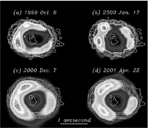
Figure 15.: ACIS images and HST contours of the emission from SNR1987A. Courtesy Dave Burrows.

Hot Pixels and Columns

Radiation damage or manufacturing defects can cause individual pixels or entire columns to have anomalously high dark current. If the dark current is large enough, the pulse height in the pixel or in an entire column can regularly exceed the event threshold and produce spurious events. These features, known as hot pixels and columns, are generally removed in data analysis. Because of the low operating temperature of $-120^{\circ}$C, which reduces dark current, there are few hot pixel and columns on the ACIS CCDs. Currently less than 1% of the entire 10 CCD focal plane are impacted and the rate of increase in these features is very small, of order a few pixels per year.

Energy Resolution

Good spectral resolution depends upon the accurate determination of the total charge deposited by a single photon. This in turn depends upon the fraction of charge collected, the fraction of charge lost in transfer from pixel to pixel during read-out typically expressed as the charge-transfer-inefficiency (CTI), and the ability of the readout amplifiers to measure the charge. Spectral resolution also depends on read noise and the off-chip analog processing electronics. The ACIS CCDs have readout noise less than 2 electrons RMS. Total system noise for the 40 ACIS  signal chains (4 nodes/CCD) ranges from 2 to 3 electrons (rms) and is dominated by off-chip analog processing electronics.

The ACIS FI CCDs originally approached the theoretical limit for energy resolution at almost all energies, while the BI were of somewhat lesser quality due to imperfections induced in the manufacturing process (Bautz et al. 1998). Subsequent to launch and orbital activation, the FI CCDs have developed much larger CTI and the energy resolution of the FI CCDs has become a function of the row number, being nearer pre-launch values close to the frame store region and progressively degraded toward the farthest row (Prigozhin et al. 2000) as shown in Figure 16.

Figure 16.: The energy resolution at 2 energies of two of the CCDs (S3 a BI CCD and I3 a FI CCD) as a function of row number for an operating temperature of $-120^{\circ}$C. The diamonds and squares are for the FI data before and after applying a post-facto correction. The solid curves are for the BI data.

The damage to the FI CCDs was caused by low energy protons, encountered during radiation belt passages, and which Rutherford-scattered from the X-ray telescope optical surfaces onto the focal plane. Subsequent to the discovery of the degradation, operational procedures were changed so that the ACIS instrument is not left at the focal position during radiation belt passages. Since then, degradation in performance has been limited to the small, gradual increase due to cosmic rays that was predicted before launch. The BI CCDs were not impacted, consistent with the proton scenario, as it is far more difficult for low energy protons to deposit their energy in the buried channels where damage is most detrimental to performance. These channels are near the CCD gates and the BI gates face in the direction opposite to the telescope.

Figures 17 and 18 show the time-dependent change in parallel (row-dependent) CTI on both FI and BI CCDs. The CTI is increasing at a rate of $3\times 10^{-6}$ yr^-1 on the FI CCDs and $1\times 10^{-6}$ yr^-1 on the BI CCDs. CTI in the serial transfer direction (column-dependent) has not increased since launch.

Figure 17.: The time-dependent change in parallel CTI at 5.9 keV for the FI CCD I3 subsequent to the proton damage early in the mission.

Figure 18.: The time-dependent change in parallel CTI at 5.9 keV for the BI CCD S3.

A post-facto software correction has been developed which can effectively recover much of the resolution lost due to the increased, row-dependent CTI (Townsley et al. 2002). For example, for the I3 FI CCD furthest from the framestore where resolution is most degraded, the FWHM is improved from 420 eV to 260 eV at 5.9 keV and from 210 eV to 150 eV at 1.5 keV, as shown in Figure 16

Many Chandra observing programs make use of ACIS spectral resolution to achieve their scientific goals. An example is shown in Figure 19 (Hwang, Holt & Petre 2000). This set of images of the supernova remnant Cassiopeia A (Cas A) was made by using the CCD energy resolution to differentiate between emission from various ions. The distinctive morphology of each image was used to study the evolving ejecta distribution and its interaction with the surrounding medium.

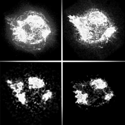
Figure 19.: Images of the supernova remnant Cas A. Upper left: Broadband X-ray image. Upper right: Image made by X-rays from silicon ions. Lower left: Image made by X-rays from calcium ions. Lower right: Image made by X-rays from iron ions. All images are 8.5 arc minutes on a side. (Credit: NASA/GSFC/U.Hwang et al. )

ACIS Time Resolution

ACIS has a multitude of operating modes which offer different time resolution. In what is referred to as the standard timed exposure mode, the CCDs collect data for a set period of time, then the imaging region of the CCD is quickly transferred (40 $\mu$sec per transfer) to the framestore to be read out. For most efficient operation, the exposure time for a CCD frame is set equal to the time required to read out the active region of the CCD. For six CCDs on and reading out the full frame, the frame time is 3.2 seconds and this is the mode which is typically used. It is possible to configure the instrument to read out smaller subarrays and/or operate fewer CCDs to reduce the frame time to a minimum of 0.2 seconds.

Higher time resolution can be obtained at the expense of one dimension of spatial resolution. In what is referred to as the continuous clocking mode, data are moved through the CCD at a rate of 3 msec per transfer. In this mode, the precise location of an event along a column is lost. On-orbit, the timing with ACIS has performed as expected.

Quantum Efficiency (QE)

The CCD quantum efficiencies for the I3 FI CCD and S3 BI CCD, convolved with the appropriate optical blocking filter, are shown in Figure 20. Characteristic absorption edges from materials in the CCD gate structures and the filter are seen at low energies. At high energies the QE is bounded by the thickness of the sensitive depletion region. The BI CCDs, whose gate structures face away from the telescope, have much higher QE at low energies, but have lower QE at high energies because they are thinner.

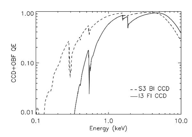
Figure 20.: Nominal ACIS quantum efficiency convolved with the optical blocking filter for the I3 FI CCD and the S3 BI CCD.

Charge transfer inefficiency degrades somewhat the uniformity of the nominal QE by redistributing the charge in an X-ray event island (an “event island” consists of an array of 3x3 or 5x5 pixels, depending on the selected mode of operation) - so that it appears more like a cosmic ray and is consequently rejected in analysis. Therefore, regions of the CCD far from the readout can have slightly lower effective QE than regions close to the readout. To date, and at the current operating temperature of $-120^{\circ}$C, the effect of CTI on quantum efficiency uniformity is small. At energies above a few keV, there is a maximum range of $\sim$ 5% - 10% in QE for the FI CCDs and a much smaller range for the BI CCDs.

Contamination

The ACIS instrument has the coldest surfaces on the Observatory. Thus, naturally, there has been a gradual accumulation of a contaminating layer since soon after launch which decreases the low energy detection efficiency and introduces distinctive absorption edges. The contaminant is believed to be deposited on the optical blocking filters and not on the CCDs themselves as there is no clear ballistic path. These filters are nominally at a temperature of -60 degrees C. Low Energy Transmission Grating (LETG - § 6.1.) observations of bright astrophysical continuum sources have been used to construct a detailed empirical model of the contaminant (Marshall et al. 2004). The dominant element in the contaminant is carbon ($>$ 80% by number and excluding hydrogen), but small edges due to oxygen (7%) and fluorine (7%) are also detectable.

Figure 21 shows the time dependent decrease in transmission from the contaminant as measured using the on-board calibration sources at 700 eV and 1.5 keV. After four years the transmission at 700 eV is about 60% of the pre-launch value and at 1.5 keV is about 93% of the pre-launch value.

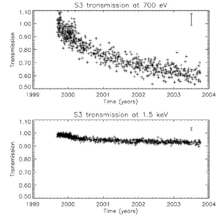
Figure 21.: The time-dependent change in transmission at 700 eV and 1.5 keV due to the deposition of a contaminant on the ACIS optical blocking filters. A typical error bar is shown in the upper right.

An obvious response to contaminant deposition is to temporarily raise the temperature of the focal plane. This procedure has not been immediately undertaken because of the experience, early in the mission, in which a bakeout further degraded the CTI of the already radiation damaged FI CCDs. Further lab studies of radiation damaged CCDs have confirmed this effect. Currently the risks and benefits of different bakeout scenarios are under study.

Background

Cosmic-ray-induced events experienced by the ACIS CCDs are very effectively minimized by on-board processing ($\sim$ 99% and $\sim$ 79% for FI and BI CCDs). The remaining background can be separated into two parts; a slowly varying quiescent component and flares in which the count rate can increase dramatically over time scales of minutes to hours (Plucinsky &Virani 2000). The quiescent background is due to high energy cosmic rays and is anti-correlated with the solar cycle. The flares show some correlation with the orientation of the Observatory’s orbit with respect to the Earth’s magnetosphere and with the Observatory’s altitude (Grant et al. 2002). The frequency and magnitude of the flares are much more pronounced in the BI CCDs than in the FI CCDs and less pronounced when either transmission grating is inserted, consistent with the suggestion that the flaring events are caused by weakly penetrating low energy protons that reach the focal plane after reflection off the telescope. The gate structure of the FI CCDs absorbs most of the protons for the majority of the flares. The spectral shape of both the quiescent and flaring background is described in more detail by Markevitch et al. (2003).

The region of the Hubble Deep Field-North was observed using the ACIS-I array, for 970 ksec in a series of twelve pointings spanning a period of 15 months and provided an excellent representation of the background and its spectrum. This spectrum, after removing the contribution from point sources, is shown in Figure 22. The prominent spectral lines in Figure 22 are from cosmic ray induced fluorescence of the gold-coated collimator, the nickel-coated substrate of the collimator, the silicon in the CCDs and from aluminum used in various places in the housing and the filter coating. In general, the background produced by the fluorescent lines is only about 2.6% of the background not found in the lines in the soft (0.5-2.0 keV) band and 13.5% of the flux in the hard (2.0-10.0 keV) band. A number of on-ground data filtering techniques have been developed which significantly suppress background. Brandt et al. (2001) have noted an approach wherein the background can be reduced by up to 36%, while only reducing source counts by 12%. Another technique, which requires a particular ACIS mode of operation, can reduce the background by 30-80% depending on the energy of interest with a minimal loss ($\sim$ 2%) of source events (Vikhlinin 2002).

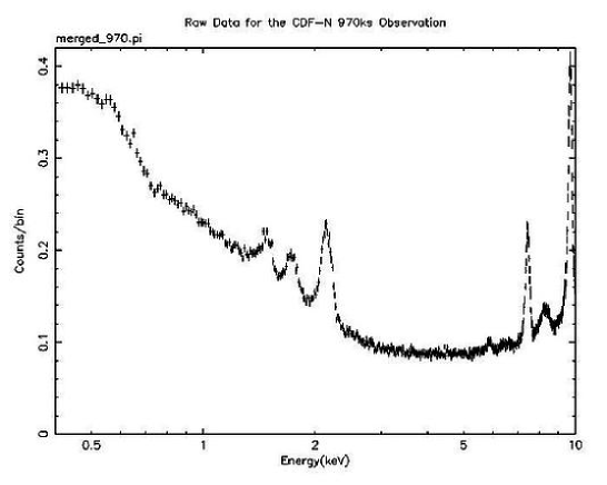
Figure 22.: A background spectrum deduced from a 970 ksec exposure to the Chandra Deep Field-North region after removing sources. The four prominent lines in order of increasing energy are Al, Si, Au, and Ni.

4.2. HRC

The Smithsonian Astophyscial Observatory (SAO, Cambridge MA), designed and fabricated the HRC (Murray et al. 2000) shown in Figure 23. Made of a single 10-cm-square microchannel plate (MCP), the HRC-I provides high-resolution imaging over a 30-arcmin-square field of view. Comprising 3 rectangular MCP segments (3-cm $\times$ 10-cm each) mounted end-to-end along the grating dispersion direction, a second detector, the HRC-S, serves as the primary read-out detector for the LETG. Both detectors have cesium-iodide-coated photocathodes and are covered with aluminized-polyimide UV/ion shields. A schematic of the HRC layout is shown in Figure 24, and a summary of the characteristics is given in Table 3.

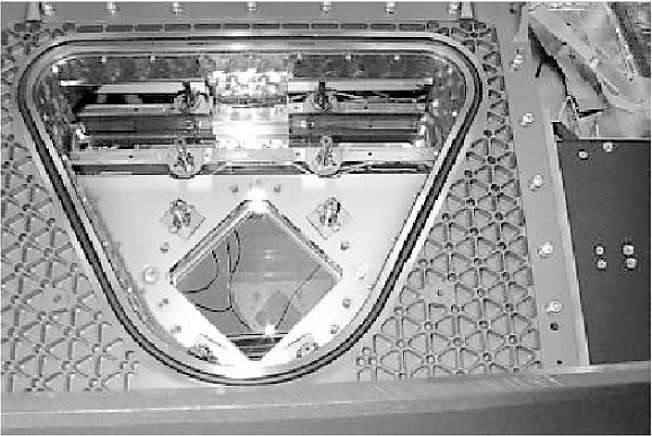
Figure 23.: Photograph of the HRC. The HRC-I (imager) is at the bottom; the HRC-S (the readout for the LETG), at the top.

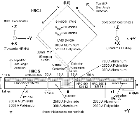
Figure 24.: A schematic of the HRC focal plane geometry as viewed along the optical axis from the telescope toward the focal plane.

Table 3.: HRC Parameters

HRC-I:	CsI-coated MCP pair	$90\times 90$ mm coated
		($93\times 93$ mm open)
HRC-S:	CsI-coated MCP pairs	3-$100\times 20$ mm
Field of view	HRC-I:	$\sim 30\times 30$ arcmin
	HRC-S:	$6\times 99$ arcmin
MCP Bias angle:		$6^{\circ}$
UV/Ion Shields:
	HRC-I:	5520 Å Polyimide, 763 Å Al
	HRC-S:
	Inner segment	2750 Å Polyimide, 307 Å Al
	Inner segment “T”	2750 Å Polyimide, 793 Å Al
	Outer segment	2090 Å Polyimide, 304 Å Al
	Outer segment (LESF)	2125 Å Polyimide, 1966 Å Al
Spatial resolution	FWHM	$\sim 20\mu$m, $\sim 0.4$ arcsec
	HRC-I: pore size	10$\mu$m
	HRC-S: pore size	12.5$\mu$m
	HRC-I: pore spacing	12.5$\mu$m
	HRC-S: pore spacing	15$\mu$m
	pixel size (electronic readout)	$6.429\mu\rm m$
		[0.13175 arcsec pixel-1]
Energy range:		$0.08-10.0$ keV
Spectral resolution	$\Delta E/E$	$\sim 1$ @1keV
MCP Quantum efficiency		30% @ 1.0 keV
		10% @ 8.0 keV
On-Axis Effective Area:	HRC-I, @ 0.1 keV	$5\,\rm cm^{2}$
	HRC-I, @ 1 keV	$227\,\rm cm^{2}$
Time resolution		16 $\mu$sec
Limiting Sensitivity	point source, 5 count detection in $3\times 10^{5}$ s	$7\times 10^{-16}\rm erg\,cm^{-2}\,s^{-1}$
	(power law spectrum: $\alpha$ = 1.4,
	$\rm N_{H}=3\times 10^{20}$ cm-2)
On-orbit	HRC-I	9$\times 10^{-6}$ cps arcsec-2
quiescent background	HRC-S	1.8$\times 10^{-4}$ cps ${\rm(res.\ elm.)^{-1}}$
(prior to ground processing)		(0.07Å$\times$ 0.1 mm)
Intrinsic dead time		50 $\mu$s
Constraints:	telemetry limit	184 cps
	maximum counts/observation/aimpoint	450000 cts
	linearity limit (on-axis point source)
	HRC-I	$\sim$ 5 cps (2 cps $\rm pore^{-1}$)
	HRC-S	$\sim$ 25 cps (10 cps $\rm pore^{-1}$)

Spatial Resolution & Encircled Energy

The intrinsic PSF of the HRC is well modeled by a Gaussian with a FWHM of $\sim 20\mu$m ($\sim$ 0.4 arcsec). The HRC pixels are $6.429~{}\mu$m (0.13175 arcsec). Approximately 90% of the encircled energy lies within a 7-pixel radius region (0.9 arcsec) from the center pixel. The image resolution with the HRC at the focus degrades off-axis as the telescope PSF increases with increasing off-axis angle and with increasing deviation between the various HRC detection surfaces and the curved telescope focal surface. Figure 25 is a spectacular example of an image made with the HRC.

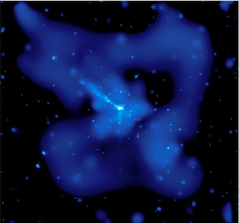
Figure 25.: HRC-I image of Centaurus A covers 30’ by 30’ and highlights the large field of view.

Energy Resolution

The pulse-height amplitude of each event is telemetered, however, the energy resolution is very poor and is not used for data analysis.

Spatial Variations

There is spatial variation in the MCP electron gain across both instruments. However, the detector quantum efficiency is unaffected by this variation as illustrated in Figure 26.

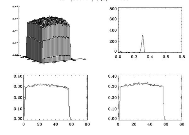
Figure 26.: HRC-I quantum efficiency as a function of position at 1.5 keV. Top left - as a function of position. Top right - distribution of quantum efficiency values. Bottom left - efficiency as a function of one spatial coordinate. Bottom right - efficiency as a function of the other spatial coordinate.

UV/Ion Shields

The placement, composition, and thickness of various UV/ion shields (filters) were shown in Figure 24. The shields are present to suppress out-of-band radiation from the ultraviolet through the visible. This suppression is particularly important for observing sources which have bright XUV and UV fluxes. The transmission of the UV/ion-shields are shown in Figures  27 and  28. The HRC/S UV/ion shields are designed to allow the center segment to be used for imaging and to allow the outer segments to detect the longer wavelengths dispersed by the LETG, up to 170Å.

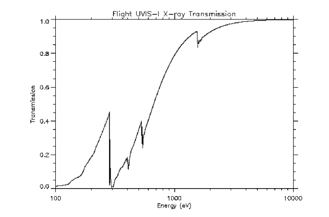
Figure 27.: The transmission of the HRC-I UV/Ion shield as a function of energy.

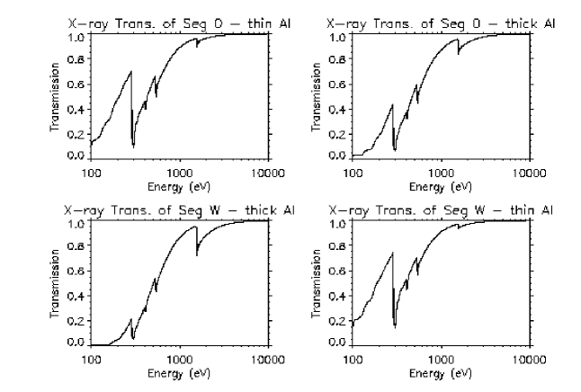
Figure 28.: The transmissions of the HRC-S UV/Ion shields for (upper left) the thin Al inner segment (seg 0); (upper right) the thick Al inner segment (seg 0, “T”); (lower left) the thick Al outer segments (“wings” or seg +1,-1); (lower right) the thin Al outer segments (“wings” or seg +1,-1).

As part of the in-flight calibration program the bright A-star Vega (A0 V, U=0.02, B=0.03, V=0.03) was observed with both HRC detectors. The predicted HRC-I count rate (assuming no X-ray emission from the star) was $7\times 10^{-4}$cps and an upper limit of $1~{}\times~{}10^{-3}$ cps was observed. The image of Vega was also placed on three regions of the HRC-S - the inner segment “T”, the thin aluminum inner segment, and on one of the thin aluminum outer segments (Figure 24). The predicted count rates were 1, 400, and 2000 cps, respectively. The corresponding observed rates were 0.2, 240, and 475 cps, well within the allowed uncertainty. The star Sirius was also observed with the HRC-S/LETG in order to obtain a soft X-ray spectrum of Sirius B (a white dwarf). Sirius A ( A1 V, V=-1.46, B-V=0.01) was seen in 0-th order at about the expected count rate. Thus, the filter is working within the accuracy of the pre-launch calibration and the performance has been stable over the first four years on-orbit.

Scattered UV, far-UV, and extreme-UV (XUV) light from the Sun or bright Earth may cause a background strongly dependent on viewing geometry. The spacecraft was designed to limit the contribution from stray scattered radiation to 0.01 ${\rm cts~{}cm^{-2}~{}s^{-1}}$ on the HRC. The imaged components of scattered radiation are dependent on the solar cycle, but are at most $\sim$ 0.01 ${\rm cts~{}cm^{-2}~{}s^{-1}}$ for most lines of sight.

Quantum Efficiency and Effective Area

The combined HRC-I and HRC-S effective areas are the product of the telescope effective area, the quantum efficiency of the HRC detectors and the transmission of the appropriate UV/Ion shield. The current best estimates of these effective areas are shown, integrated over the point spread function, in Figure 29.

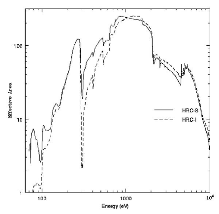
Figure 29.: The telescope/HRC-I (dashed) and the center section of the telescope/HRC-S (solid) effective area as a function of energy, integrated over the PSF. Absorption edges are due to the iridium on the mirror, the CsI coating, and the polyimide/Al UV/Ion shield.

On-Orbit Background

HRC-I

The raw HRC-I counting rate on orbit is about 250 cps total. These are mostly cosmic ray events which are also detected in the anti-coincidence shield. After anticoincidence, the valid event rate is about 50 c/s over the field yielding a background rate of 10^-5 ${\rm cts~{}s^{-1}~{}arcsec^{-2}}$. The background is generally flat, or at least smoothly varying over the field with no more than a 20% difference between the center (higher rate) and edges (lower rate) of the detector.

HRC-S

The anti-coincidence shield of the HRC-S is not working because of a timing error in the electronics. As a result the event rate is very high and would exceed the total telemetry rate limit, thus impacting observing efficiency. To cope with this problem, on-board data collection is limited to a region which is about 1/2 of the full width and extends along the full length of the detector. With this change, the quiescent background rate is about 85 cps.

Both HRC detectors experience occasional fluctuations in the background due to variations in the charged particle background. These times of enhanced background are typically short (a few minutes to a few tens of minutes) and are anywhere from a factor a 2 to a factor of 10 over the quiescent rate. The increased background appears to be uniformly distributed over the detector and introduces no apparent image artifacts.

Ghost Images

There is a very faint “ghost” image displaced 10 arcsec on one side of every source in the field of view in the HRC-I. These ghost images are due to events where the electronic signals saturate one or more amplifiers in the event processing chain. An event processing algorithm has been developed that eliminates the bulk of this spurious image. The intensity of the ghost is $<3$% of the source signal without filtering and $<0.1$% after filtering. The same feature is present in the HRC-S, but at a much reduced intensity.

HRC Timing

The HRC time resolution of 16 $\mu$sec offers the highest precision timing of the two imaging cameras. However, the HRC was mis-wired so that the time of the event associated with the j-th trigger is that of the previous (j-th -1) trigger. If the data from all triggers were routinely telemetered, the mis-wiring would not be problematical and could be dealt with by simply reassigning the time tag. Since the problem has been discovered, new operating modes have been defined which allow one to telemeter all data whenever the total counting rate is moderate to low, albeit at the price of higher background. For very bright sources the counting rate is so high that information associated with certain triggers are never telemetered. In this case, the principal reason for dropping events is that the on-board, first-in-first-out (FIFO) buffer fills as the source is introducing events at a rate faster than the telemetry readout. Events are dropped until readout commences freeing one or more slots in the FIFO. This situation can also be dealt with (Tennant et al. 2001) and time resolution of the order of a millisecond can be achieved.

An example of the excellent timing performance of the HRC-S (Imaging) mode is seen in the light curve for 3C58 (Murray et al. 2002) shown in Figure 30. 3C58 is a supernova remnant with a central compact source which was suspected to be a pulsar, but for which no pulsations had been previously observed. A Chandra -HRC-S observation showed the pulse period to be about 65 msec and the pulse profile to consist of a very short main pulse (a few msec wide) and a somewhat broader interpulse.

Figure 30.: Light curve of the pulsing X-ray source in 3C58.

More details of the HRC and its performance may be found in Murray et al. 2000, Kenter et al. (2000), and Kraft et al. (2000).

5. Electron Proton Helium Instrument (EPHIN)

Mounted on the spacecraft and near the X-ray telescope is a particle detector: the Electron, Proton, Helium INstrument (EPHIN). The EPHIN instrument was built by the Institut für Experimentelle und Angewandte Physik, University of Kiel, Germany, and a forerunner was flown on the SOHO satellite.

EPHIN consists of an array of 6 silicon detectors with anti-coincidence. The instrument is sensitive to electrons in the energy range 250 keV - 10 MeV, and hydrogen and helium isotopes in the energy range 5 - 53 MeV/nucleon. Electrons above 10 MeV and nuclei above 53 MeV/nucleon are registered with reduced capability to separate species and to resolve energies. The field of view is 83^o with a geometric factor of 5.1 cm² sr.

EPHIN is used to monitor the local charged particle environment as part of the scheme to protect the focal-plane instruments from particle radiation damage. EPHIN is also a scientific experiment in its own right. A detailed instrument description is given in Mueller-Mellin et al. (1995).

6. Gratings

Aft of the X-ray telescope are 2 objective transmission gratings (OTGs) - the Low-Energy Transmission Grating (LETG) and the High-Energy Transmission Grating (HETG). Positioning mechanisms are used to insert either OTG into the converging beam where they disperse the x-radiation onto the focal plane. Figure 31 shows the gratings mounted behind the X-ray telescope in their retracted position.

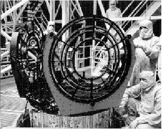
Figure 31.: Photograph of the LETG and HETG mounted to the spacecraft structure. Photograph is from TRW.

6.1. LETG

The Space Research Institute of the Netherlands (SRON, Utrecht, Netherlands) and the Max-Planck-Institüt für extraterrestrische Physik (MPE, Garching, Germany) designed and fabricated the LETG. The LETG is a slitless spectrometer employing a Rowland geometry. The diffraction grating itself is comprised of 540 individual gold grating elements held in place by an aluminum structure designed such that the individual elements form parts of the surface of a Rowland torus. The individual grating facets are circular with a diameter of approximately 1.6 cm. Each facet consists of bars with $0.5\mu\times 0.5\mu$ square cross-section, held in place by a fine perpendicular grid of thicker bars and a triangular lattice. The main characteristics of the LETG are summarized in Table 4.

The LETG is put into operation by rotating the holding structure into its place in the light path about 300 mm behind the exit aperture of the telescope. The 540 grating facets, mounted 3 per module, then lie tangent to the Rowland toroid which includes the focal plane. With free-standing gold bars of about 991-nm period, the LETG provides high-resolution spectroscopy ($E/\Delta E$ $>1000$) between 80 and 175 Å (0.07 – 0.15 keV) and moderate resolving power at shorter wavelengths. The nominal LETG wavelength range accessible with the HRC-S as the detector is 1.2 – 175 Å (0.07 – 10 keV); ACIS-S coverage is 1.2 – 65 Å (0.20 – 10 keV).

Table 4.: LETG Parameters

Rowland diameter	$8637$ mm
LETG grating parameters
Period	0.99125 $\pm 0.000087$ $\mu$m
Thickness	0.474 $\pm 0.0305$ $\mu$m
Width	0.516 $\pm 0.0188$ $\mu$m
Fine-support structure
Period	25.4$\mu$m
Thickness	2.5$\mu$m
Coarse-support structure
Triangular height	2000$\mu$m
Width	68$\mu$m
Thickness	$<30\mu$m
Instrument Bandpass	1.2-175 Å (70-10000 eV) (HRC-S)
	1.2-65 Å (200-10000 eV) (ACIS-S)
Resolution ($\Delta\lambda$, FWHM)	$0.05$ Å
Resolving Power ($\lambda/\Delta\lambda$)	$\geq 1000$ (50–160 Å)
	$\approx 20\times\lambda$ (3-50 Å)
Dispersion	1.148 Å/mm
Detector angular size	3.37’ $\times$ 101’ (HRC-S)
	8.3’ $\times$ 50.6’ (ACIS-S)
Temporal resolution	16 $\mu$sec (HRC-S in Imaging Mode, center segment only)
	$\sim$10 msec (HRC-S in default mode)
	2.85 msec–3.24 sec (ACIS-S, depending on mode)

The on-orbit performance of the LETG is similar to pre-flight predictions (e.g. Brinkman et al. 1997; Predehl et al. 1997; Dewey et al. 1998), though some minor problems with the readout detectors have provided challenges for data analysis and the implementation of some observations. These are: (i) a high HRC-S background rate resulting from inoperability of anti-coincidence veto of energetic particle events; (ii) small-scale spatial non-linearity in HRC-S event position determination; (iii) the build-up of a contamination layer on the ACIS-S filter that significantly reduces the effective area of the LETG+ACIS-S combination for wavelengths longward of $\sim 18$ Å ($\sim 0.7$ kev); all of which were discussed previously in § 4.1. and  4.2.

The capabilities and usage of the LETG gratings are defined by their spectral resolution and energy range. From an astrophysical perspective, salient attributes include: the ability to study the very softest X-ray sources at high spectral resolution, such as hot white dwarfs, novae, and isolated neutron stars, whose radiative output peaks at wavelengths longward of 20 Å or so ($\sim 0.6$ keV); coverage of two decades in wavelength such that the precise shapes of the spectral energy distributions of sources with strong non-thermal emission components can be investigated, including intervening absorption systems; inclusion of the resonance lines of all of the astrophysically important C, N and O trio for study in emission and absorption; the highest spectral resolving power Chandra has to offer, reaching $\lambda/\Delta\lambda\sim 2000$ at $\mathrel{\hbox{\hbox to0.0pt{\hbox{\lower 4.0pt\hbox{$\sim$}}\hss}\hbox{$>$}}}100$ Å; and simultaneous spectroscopy and high time resolution using the HRC-S detector (§ 4.2.).

Dispersion Relation

The dispersive properties of the LETG are calibrated and monitored in-flight using the spectra of stellar coronae. The primary calibration target is the evolved binary Capella (G2 III+G8III). While not ideal from the standpoint of being a binary - the projected orbital speed of the two components is 36 km s^-1 and can cause discernible shifts and broadening of spectral lines at Chandra’s highest resolution - Capella is the brightest coronal X-ray source in the sky and provides calibration information with the minimum of observing time.

Stellar coronal spectra are dominated by emission lines from highly ionized astrophysically abundant elements—predominantly C, N, O Ne, Mg, Si, Ar and Fe. Shortward of 40 Å (0.3 keV) or so, the H-like and He-like ions of these elements provide resonance lines with very precisely calculated wavelengths that are ideal for examining and monitoring dispersion relations. In principle, these lines can be supplemented with the forest of Fe lines from the “L-shell” complex (transitions among valence electrons with n=2 ground states). However, at the LETG resolution of up to $\lambda/\Delta\lambda\sim 2000$, many of the wavelengths of these lines are known much less precisely and must be treated with caution. Longward of 40 Å  laboratory wavelengths of light element L-shell lines and transitions of the type $\Delta n=0$ in Fe L-shell ions provide the wavelength benchmarks. Before use in calibration, lines are first screened based on spectrum synthesis-type calculations for the presence of significant blends that might skew the observed wavelengths from their true values.

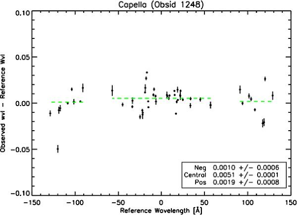
Figure 32.: The difference between observed and theoretical wavelengths as a function of wavelength for relatively unblended spectral lines in the coronae of Capella, seen by the LETG+ACIS-S (top), LETG+HRC-S (bottom). Small departures from zero are expected based on the residual orbital velocities and on the presence of hidden blends. In the case of the HRC-S, however, the much larger departures are cause by imaging non-linearities in the detector.

The current LETG dispersion relations with the HRC-S and ACIS-S detectors as illuminated by Capella (after correction for the spacecraft and Capella systemic radial velocity differences) are shown in Figure 32. In the case of ACIS-S, the RMS deviation in predicted vs. observed line wavelength amounts to only $\sim 0.002$ Å or 0.01 %. The scatter seems larger than the errors bars suggest should be the case; this is likely due primarily to hidden line blends. To put these results in perspective, the net orbital velocity of the Capella components is of a similar magnitude and, ultimately, we do not know from which binary component the lines are emitted.

In the case of the HRC-S the RMS deviation between observed and predicted wavelengths for the set of relatively unblended lines observed amounts to 0.013 Å—almost an order of magnitude higher than with ACIS-S, though at 100 Å this again amounts to an effect of order 0.01% . Close examination of Figure 32, however, reveals especially large departures, especially at wavelengths falling on the outer HRC-S plates, and on the central plate near 20 Å. These differences between predicted and observed wavelengths have been found to be caused by small non-linearities in the imaging characteristics of the detector. These are understood in terms of small errors in the positions of events, as determined by the combination of detector electronics and ground telemetry processing. Correcting for these small position errors is not trivial and future improvements to the dispersion relation will rely on empirical corrections based on a large accumulation of data such as that in Figure 32.

Resolving Power

The dominant contribution to the LETG line response function (LRF) and instrument resolving power is the telescope PSF, which is $\sim 25~{}\mu$m FWHM, depending on energy. When the LETG is used with the HRC-S, the intrinsic uncertainty in photon position determination adds another small contribution of order 15-$20~{}\mu$m. The LETG itself does not contribute any significant broadening. Uncertainties in correcting photon event positions for the observatory aspect, which occurs during ground data processing, also introduces an additional, but small, blurring of order a few $\mu$m. For spectral lines with $\mathrel{\hbox{\hbox to0.0pt{\hbox{\lower 4.0pt\hbox{$\sim$}}\hss}\hbox{$<$}}}1000$ counts, the combined LETG+HRC LRF can be well-approximated by the function

$$I(\lambda)={[1+\left({\lambda\over{\lambda_{c}}}\right)^{2}]^{-\beta}}$$ (1)

with FWHM$\sim 40$ $\mu$m, or $\sim 0.05$ Å. The LETG resolving power determined by fitting this function to lines seen in spectra of Capella and Procyon is illustrated in Figure 33, together with pre-flight model predictions.

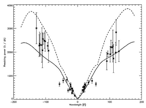
Figure 33.: LETG/HRC-S spectral resolving power derived from lines thought not to be affected significantly by blending from several observations of Capella and Procyon. Measured line widths were corrected for source orbital, rotational, and thermal motions. Optimistic (dashed line) and conservative (solid line) predictions of pre-flight models are also shown. The deviations from approximate linearity near $\pm 60$ Å and at the longest wavelengths arise from deviations of the HRC-S surface from the Rowland circle. Deviations from a smooth curve are likely caused by hidden blends not predicted by the radiative loss model, or by imaging non-linearities of the HRC-S along the dispersion axis.

That the current LETG LRF is now quite well-described has recently been demonstrated by Ness et al. (2003), who have succeeded in modeling the spectrum of Capella in the extremely complex 13-14 Å region that contains the He-like Ne density-sensitive lines. At the LETG resolution, these lines are heavily blended with Fe lines - predominantly Fe XIX. This spectral region cannot simply be modeled based on optically thin radiative loss models because the exact placement of the Fe lines is crucial, and model wavelengths are not of sufficient accuracy. Ness et al. (2003) circumvented this problem by examining in detail the same spectral region as seen using the HETG (§ 6.2.), in which individual blending lines could be empirically identified and isolated. Using the HETG-derived line list, and relative intensities, Ness et al. (2003) reconstructed the LETG spectrum and were able to produce an impressive fit to the observations as illustrated in Figure 34.

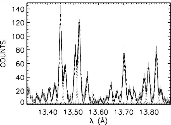
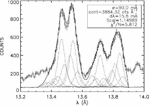
Figure 34.: Top: HEG summed plus and minus first order spectrum of Capella in the 13-14 Å range, fitted with a model comprised of 18 emission lines and a constant continuum. Bottom: The best-fit model obtained from the HEG spectrum, scaled and overlaid on the LETG spectrum. The scaling parameters are listed in the top right inset. From Ness et al. (2003).

While the LETG LRF is slightly broader than a Gaussian of the same FWHM away from line center, a key characteristic is this rather modest extension of the line wings. This greatly aides the sensitivity of the instrument: overlapping line wings are a source of noise for understanding a true continuum level, or for extracting line fluxes. One example where this sensitivity was crucial is the detection of narrow line absorption in the spectrum of the blazar PKS2155-304 by Nicastro et al. (2002), illustrated in Figure 35. O VII K_α and Ne IX K_α resonant absorption lines were detected, together with a more tentative identification of absorption due to O VIII K_α and O VII K_β. In the same line-of-sight toward PKS 2155-304, the Far Ultraviolet Spectroscopic Explorer spectrum shows complex O VI 2s2p absorption, including one significantly blue-shifted component. Nicastro et al. (2002) interpreted the combined X-ray and UV data in terms of absorption in a low-density intergalactic plasma collapsing toward our Galaxy. The presence of such an absorber had been predicted by numerical simulations of the warm-hot intergalactic medium (e.g. Hellsten et al. Kravtsov 1998; et al. 2002). Detecting these shadows of our local Universe is extremely difficult even with observatories such as Chandra - the absorption features are relatively weak, and narrow. A spectrometer such as the LETG is required: one with high spectral resolution, a sharp, well-defined instrumental profile, and with sufficient sensitivity throughout the soft X-ray range to accumulate high continuum signal from the background source.

Figure 35.: The LETG/HRC-S spectrum of PKS 2155-304 in the 11-24 Å range illustrating the continuum (well-described by a power law with Galactic absorption), together with six absorption lines (solid line). The apparent continuum shape reflects the instrument response. Four portions of the spectrum are magnified: (b) O VII K; (c) atomic and solid-state (i.e., molecular) O I; (d) Ne IX K; (e) O VII K and O VIII K.

Bandpass and Effective Area

The first order effective areas of the LETG with both HRC-S and ACIS-S detectors is illustrated in Figure 36. Toward the short wavelength limit of $\sim 1.2$ Å ($\sim 10$ keV), the area is limited by the rapidly falling reflectivity of the telescope combined with the decreasing efficiency of first order diffraction — the LETG grating bars become effectively transparent to such short wavelength photons. Both LETG/ACIS-S and LETG/HRC-S effective areas are characterized by a step near 6 Å, corresponding to the increase in reflectivity of the X-ray telescope longward of the Ir M edges. This peak is accentuated by a peak in first order diffraction efficiency. Toward longer wavelengths, both the LETG diffraction efficiency and the X-ray telescope reflectivity are essentially flat, and the shapes of the effective area curves are dominated by the transmittance of the detector filters and the detector quantum efficiencies, including any contamination. Easily visible in these curves are the absorption edges of C, N and O, that are major constituents of the polyimide filters.

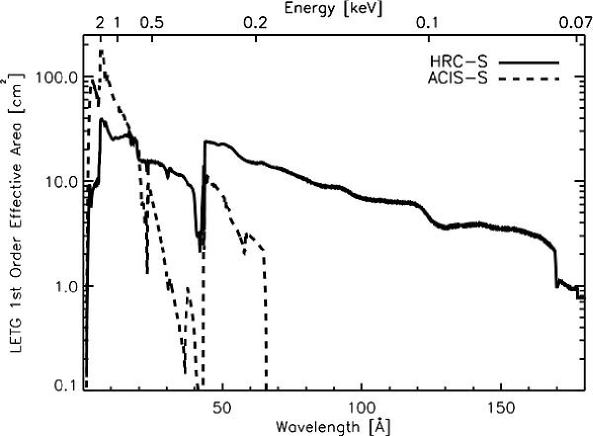
Figure 36.: Chandra LETG/HRC-S and LETG/ACIS-S first-order effective areas as a function of wavelength and energy.

With the HRC-S detector, the nominal LETG long wavelength cut-off is 170 Å (0.07 keV). This limit is simply a dictate of the physical extent of the detector. It is interesting that the Al coating of the HRC-S UVIS becomes more transparent longward of the Al L edges near 170 and 171 Å, and, by acquiring a target at an off-set position along the dispersion axis and at a small cost in resolution, the wavelength coverage can actually be stretched beyond 170 Å. A spectrum of the late-type subgiant Procyon (F5 IV) was obtained in this way and is compared in Figure 37 with the same spectral region observed by the Extreme Ultraviolet Explorer (EUVE).

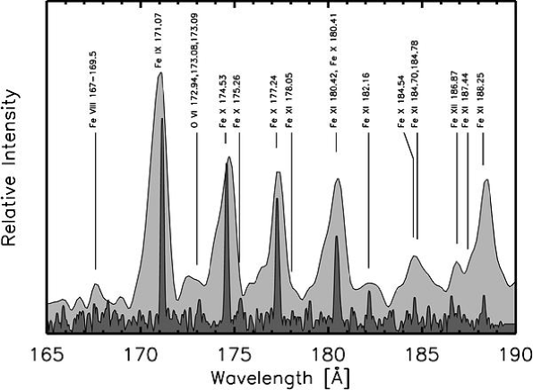
Figure 37.: Chandra LETG and EUVE Medium Wavelength Spectrometer spectra of the 165-190 Å range in Procyon (F5 IV). The Chandra spectrum was obtained with the target off-axis in the LETG dispersion direction so as to extend the wavelength range. The prominent lines are due to intermediate charge states of Fe.

In order to interpret spectra correctly over the whole of the soft X-ray range—covering two orders of magnitude in photon energy—instrumental calibration becomes a vital concern. The LETG/HRC-S effective area calibration has been adjusted post-launch based on the observed spectra of “well understood” cosmic sources and on cross-calibration with the other Chandra instruments, and is believed to be accurate to 15% or so (absolute) in first order. Marshall et al. (2003) were able to match the LETG+HRC-S spectrum of Mkn 478 with a pure continuum model from 1.2-100 Å, applying only minor adjustments to the contributions from higher spectral orders that are mixed in with the first order signal. Mkn 478 lies in a direction out of the galaxy that has a particularly low neutral hydrogen column density, and so remains a strong source at these longer wavelengths. The first order spectrum is illustrated in Figure 38. Using these data Marshall et al. (2003) argued for the absence of both a strong warm absorber, as expected based on other Seyfert 1 observations (see §7.) and a lack of emission lines at longer wavelength that were predicted based on an analysis of earlier EUVE spectra (Hwang & Bowyer 1997).

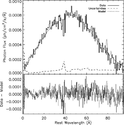
Figure 38.: First order LETG+HRC-S spectrum of Mrk 478 binned at 0.5 Å (top) and residuals from the best-fit power-law model. Residuals near the C-K edge in first order most likely result at least partly from systematic errors in the effective area calibration. The continuum appears bereft of line absorption or emission features, contrary to the expectations of Hwang & Bowyer (1997) based on their analysis of EUVE spectra. The particular lines suggested as being present in EUVE spectra by Hwang & Bowyer (1997) are included in the model in the top panel (but were not used to calculate the residuals in the bottom panel).

6.2. HETG

The Massachusetts Institute of Technology (MIT, Cambridge, Massachusetts) designed and fabricated the HETG. The HETG employs 2 types of grating facets — the Medium-Energy Gratings (MEG), mounted behind the X-ray telescope’s 2 outermost shells, and the High-Energy Gratings (HEG), mounted behind the X-ray telescope’s 2 innermost shells. With polyimide-supported gold bars of 400-nm and 200-nm periods, respectively, the HETG provides high-resolution spectroscopy from 0.4 to 4 keV (MEG, 30 to 3 Å) and from 0.8 to 8 keV (HEG, 15 to 1.5 Å).

There are 192 medium energy gratings (MEGs), each about 25 mm square, that intercept rays from the outer telescope shells and are optimized for medium energies. There are 144 high energy gratings (HEGs), also 25 mm square, that intercept rays from the two inner shells and are optimized for high energies. Both gratings are mounted on a single support structure and therefore used concurrently. The two sets of gratings are mounted with their grating bars at different angles so that the dispersed images from the HEG and MEG will form a shallow $X$ centered on the undispersed (zeroth order) position; one leg of the $X$ is from the HEG, and the other from the MEG (see Canizares et al. 2000 and Figure 39). The HETG is designed for use with the spectroscopic array of ACIS-S, although other detectors may be used for particular applications. Here we restrict the discussion to use with ACIS-S.

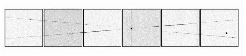
Figure 39.: The X-ray image of the HETG spectrum of Capella. The image of the flux dispersed by the MEG is in the line extending from the lower left to the upper right. The bright dot in the center is the image of the zeroth order. The bright square to the right is the effect of a bright pixel and the dither motion.

The gratings are electroplated gold bars supported on polyimide membranes. The heights and widths of the bars were chosen to maximize the efficiency into first order and reduce the zeroth order throughput. Setting the bar width to half of the grating period suppresses even orders and improves first order efficiency for rectangular bar profiles. This nulling of even orders is achieved in the MEGs. For the HEGs, the bar height was increased in order to improve the first order efficiency above 1.2 keV where the gold becomes partially transparent. In this case the fabrication process produced bar widths that were 60% of the period. A consequence is that the second order efficiency is comparable to that in third order. The MEG and HEG efficiency for the zeroth, first, second, and third orders are shown as a function of energy in Figure 40. A summary of HETG characteristics is given in Table 5.

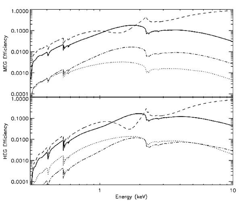
Figure 40.: The MEG (top) and HEG (bottom) dispersion efficiencies as a function of energy for orders 0 (dashed), 1 (solid), 2 (dotted), and 3 (dash-dot).

Table 5.: HETG Parameters

	HEG	MEG
HETG Rowland Spacing	$8632.65$ mm
HETG Effective Area	$28\rm\,cm^{2}$ @ 6.5 keV
(MEG+HEG first orders,	$200\rm\,cm^{2}$ @ 1.5 keV
with ACIS-S )	$59\rm\,cm^{2}$ @ 1.0 keV
Energy Range	$0.8-10.0$ keV	$0.4-5.0$ keV
Wavelength Range	$1.2-15$ Å	$2.5-31$Å
Resolving Power ($E/\Delta E$)	$1070-65$	$970-80$
Resolution (FWHM, Å)	$0.012$ Å FWHM	$0.023$
Absolute Wavelength Accuracy (Å)	$\pm 0.006$	$\pm 0.011$
Relative Wavelength Accuracy (Å)	$\pm 0.0028$	$\pm 0.0055$
Angle on ACIS-S (∘)	$-5.235\pm 0.01$	$4.725\pm 0.01$
Wavelength Scale (Å / ACIS pixel)	0.0055595	0.0111185
Diffraction Efficiency, 0.5 keV	1.4%	3.6%
($\pm$1 orders), 1.5 keV	22%	32%
6.5 keV	17%	13%
HETG Zeroth-order Efficiency at 0.5 keV	4.5%
1.5 keV	8%
6.5 keV	60%
Grating Facet Parameters
Bar material	Gold	Gold
Period (Å)	2000.81	4001.41
Bar thickness (Å)	5100	3600
Bar width (Å)	1200	2080
Polyimide support thickness (Å)	9800	5500

Imaging

The zeroth order image is not significantly degraded from that without the HETG in place. The HETG/ACIS-S in zeroth order was used to view and discover the fascinating spatial structure in the X-Ray emission from the Crab Nebula as shown in the now famous image - Figure 41 (Weisskopf et al. 2000).

Figure 41.: HETG/ACIS-S zero-order image of the central 200” x 200” of the Crab Nebula.

Wavelength Accuracy

The relative wavelength accuracy is determined by the placement of the CCDs and the accuracy of the dispersion scale, which, in turn, is set by the HEG and MEG grating periods and the distance from the grating assembly to the focal plane. The locations of the CCDs were precisely established in flight using emission lines from the calibration source Capella. The location of the CCD gaps are accurate to 0.011 Å (0.006 Å) based on measurements with the MEG (HEG) (Marshall, Dewey, & Ishibashi, 2004). The net result is that the wavelengths are typically accurate to better than 100 km/s as shown in Figure 42

Figure 42.: Measurements of lines in one observation of Capella (observation ID 2583). Open squares: Lines from the HEG portion of the spectrum. Open diamonds: Lines from the MEG portion of the spectrum. The average wavelength error is seen to correspond to velocity erros of less than 100 km/s.

Line Response Function and Spectral Resolution

The HETGS LRF has a Gaussian-like core with extended wings. The model of the HETG LRF is comprised of two Gaussians and two Lorentzians with the narrow Gaussian dominating as shown in Figure 43. The LRFs derived from the fits match in-flight data extremely well as shown in Figure 44 (Marshall, Dewey, & Ishibashi, 2004). The spectral resolution is the FWHM of the LRF and is essentially independent of wavelength and is 0.012Å for the HEG and 0.023Å for the MEG.

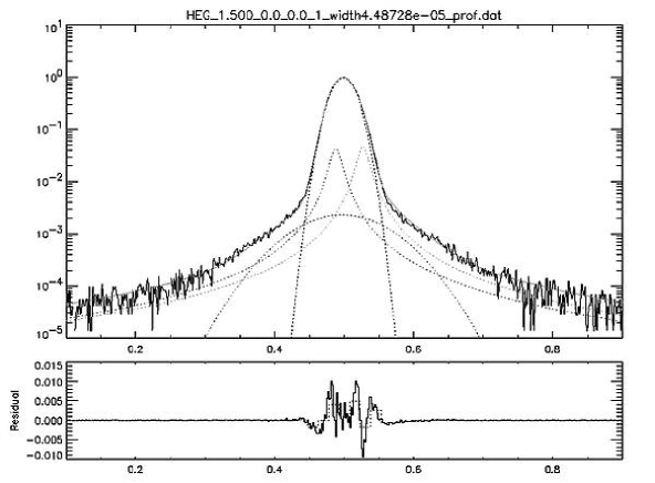
Figure 43.: Decomposition of the HETG LRF and a comparison with simulated data. This example is for the HEG in positive first order. The LRF is modeled with narrow and broad Gaussians and two Lorentzian’s, one for each of the wings to allow for asymmetry. The narrow Gaussian dominates the LRF and the Lorentzian wings are rarely detectable in flight data. The residuals (bottom panel) are largest in the core, but are not statistically significant.

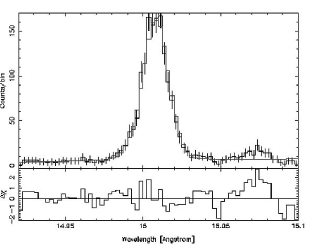
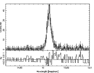
Figure 44.: Comparison of data from Capella and the LRF model for the Fe XVII line at 15.013 Å. The fit to the MEG (HEG) data is on the left (right).

Effective Area

There are many ingredients in the effective area of the HETG/ACIS-S combination. These include the telescope, the gratings and the various CCD detectors and their filter. The first order effective areas for the HEG and MEG, after adjusting the BI CCDs quantum efficiency to agree with that inferred for the FI CCDs, and accounting for the molecular contamination of the ACIS filter as of the end of 2003, is shown in Figure 45. This effective area was used to analyze the spectrum of the BL Lac object, PKS 2155-304. This object is a Chandra calibration source and its spectrum is assumed to be featureless. Figure 46 shows the results of the analysis of an observation taken in May of 2000. There are no systematic residuals larger than 10% and the spectrum appears featureless at the 3% level.

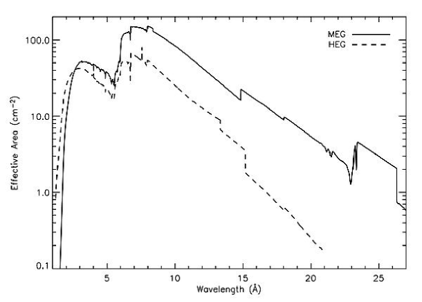
Figure 45.: First Order effective area of the HETG/ACIS-S combination accounting for contamination at the end of 2003.

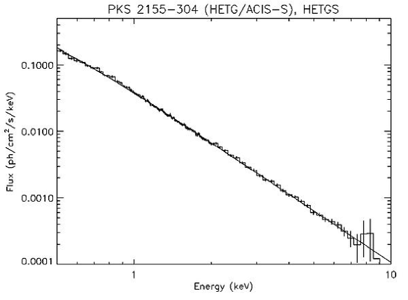
Figure 46.: HETGS spectrum of PKS 2155-304 taken in May of 2000. The data were fit to a broken (double) power model; systematic deviations are consistently less than 10%.

An example of spectroscopy with the HETG is shown in Figure 47 which shows two HETG/ACIS-S spectra (Marshall, Canizares, & Schulz, 2002; Lopez et al. 2004) of the binary source SS 433 taken at different times in the binary period. The spectra are dominated by strong emission lines on a moderately strong continuum. Here the lines are associated with the oppositely directed, mildly relativistic jets that precess with a period of 164 days (Margon et al. 1977; Abell & Margon, 1979). Marshall, Canizares, & Schulz (2002) showed that the emission lines are collisionally excited and consistent with a model of an adiabatically expanding outflow cooling from $10^{8}$K to $<10^{7}$K. Additionally, the electron density of the jet was estimated to be 10¹⁴ cm^-3 by measuring the ratio of the intercombination and forbidden lines of the Si xiii triplet, which in turn provided an estimate for the size of the jet.

The lines from the approaching (blue) jet in the first observation were strong enough to show that the resolved lines had a common blueshift, indicating that the jet was produced in a uniform conical outflow. The Doppler broadening of the lines gave the opening angle of the jet, 1.2^o. The March 2001 observation took place during orbital eclipse, and the modeling of the red jet by Lopez et al. (2004) found that the visible portion of the jet was $\sim 10^{11}$ cm long. Using the system geometry and some system parameters derived from optical observations of the accretion disk, these authors estimated that the mass of the compact object in SS 433 is about 16 $M_{\hbox{$\odot$}}$, confirming that it is indeed a black hole.

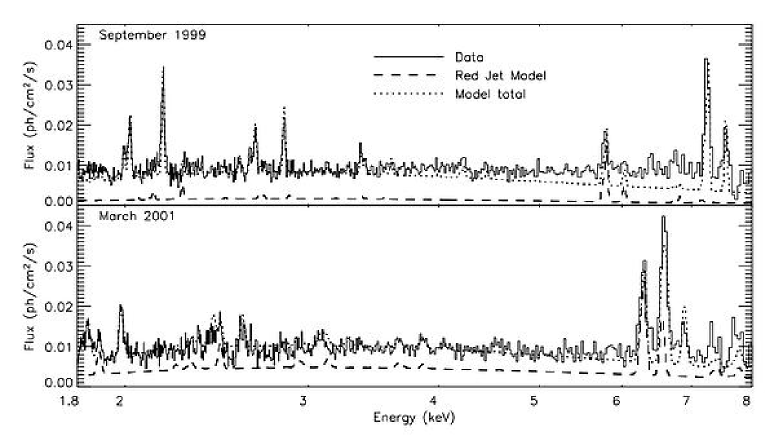
Figure 47.: HETG/ACIS-S spectra of SS 433. These spectra are rich in red- and blue-shifted emission lines from highly ionized elements: Si, S, Ar, Ca, and Fe near 2.1, 2.8, 3.5, 4.3, and 6-7 keV, respectively. The dashed lines are models of the red jet and the dotted lines are the sum of the models for the blue and red jets. Top: The spectrum obtained in September 1999 shows strong and narrow lines from the blue jet but the lines from the red jet are weak. Bottom: The spectrum obtained in March 2001 shows much stronger lines from the red jet and all lines are broader than in the earlier observation.

Another example of spectroscopy with the HETG was its use to begin to determine the abundances and ionization fractions of gas in the interstellar medium (ISM). Juett, Schulz, & Chakrabarty (2004) presented highly resolved spectra of the oxygen $K$-shell interstellar absorption edge using X-ray binaries as sources (Figure 48). The $K\alpha$ and $K\beta$ absorption lines from neutral, singly, and doubly ionized oxygen were identified as well as expected absorption edges. The observed wavelength of O I $K\alpha$ absorption line was used to adjust the wavelength of the theoretical predictions of the absorption cross sections. Juett, Schulz, & Chakrabarty (2004) also placed a limit on the velocity dispersion of the neutral lines of $\leq$200 km s^-1, consistent with measurements at other wavelengths. Finally, the HETG measurements determined the oxygen ionization fractions in the ISM in these lines of sight. This work demonstrated the utility of X-ray spectroscopy for studies of the ISM and future work with the Observatory will provide measurements of the relative abundances and ionization fractions for elements from carbon to iron for many different lines of sight.

Figure 48.: Absorption spectra in the vicinity of the oxygen K edge for Cyg X-2 (top) and Cyg X-1 (bottom) with line identifications. These data were used to measure the neutral and ionized oxygen abundances along two lines of sight in the interstellar medium (Juett, Schulz, & Chakrabarty 2004).

7. Additional Discoveries

The first X-rays focused by the telescope were observed on August 12, 1999. Figure 41 showed one of the early images. This image of the Crab Nebula and its pulsar included a major new discovery (Weisskopf et al. 2000) - the bright inner elliptical ring showing the first direct observation of the shock front where the wind of particles from the pulsar begins to radiate in X-rays via the synchrotron process. Discoveries of new astronomical features in Chandra images have been the rule, not the exception.

The Observatory’s capability for high-resolution imaging enables detailed studies of the structure of extended X-ray sources, including supernova remnants, astrophysical jets, and hot gas in galaxies and clusters of galaxies. Equally important are Chandra’s unique contributions to high-resolution dispersive spectroscopy. As the capability for visible-light spectroscopy initiated the field of astrophysics about a century ago, high-resolution X-ray spectroscopy now contributes profoundly to the understanding of the physical processes in cosmic X-ray sources and is the essential tool for diagnosing conditions in hot plasmas. The high spectral resolution of the Chandra gratings isolates individual lines from the myriad of spectral lines, which would overlap at lower resolution. The additional capability for spectrometric imaging allows studies of structure, not only in X-ray intensity, but also in temperature and in chemical composition. Through these observations, users are addressing several of the most exciting topics in contemporary astrophysics.

In addition to mapping the structure of extended sources, the high angular resolution permits studies of discrete sources, which would otherwise be impossible. An example is shown in Figure 49 where one sees X-rays produced by TWA 5B, a brown dwarf orbiting a young binary star system known as TWA 5A6. This observation not only demonstrates the importance of the Chandra angular resolution but also addresses the question as to how do brown dwarfs heat their upper atmospheres (coronas) to X-ray-emitting temperatures of a few million degrees.

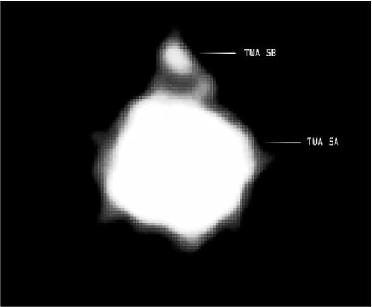
Figure 49.: X-rays produced by TWA 5B, a brown dwarf orbiting a young binary star system known as TWA 5A. The image is 6-arcsec on a side. Courtesy of NASA/CXC/Chuo U.

From planetary systems to deep surveys of the faintest and most distant objects, the scientific results from the first years of Chandra operations have been exciting and outstanding. We conclude this paper with an overview of some of these results.

We begin with images of the X-ray emission from the planet Jupiter. Figure 50 shows hot spots at high (and unexpected) latitudes that appear to pulsate at approximately a 45-minute period (Gladstone et al. 2002). In this case the X-rays appear to be produced by particles bombarding the Jovian atmosphere after precipitating along magnetic field lines. Figure 51 continues the discoveries about the Jovian system and shows the first detection of X-rays from two of the moons – Io and Europa (Elsner et al. 2002).

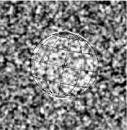
Figure 50.: Chandra image of Jupiter showing the hot spots at high latitudes. The image is 50–arcsec on a side. Courtesy R. Elsner.

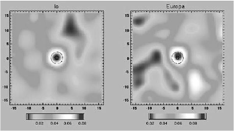
Figure 51.: Chandra images of the Jovian moons Io and Europa. Courtesy R. Elsner.

In Figure 52 we show a more recent detection (Dennerl, 2002) of fluorescent scattering of solar X-rays in the upper atmosphere of Mars. The X-ray spectrum is dominated by a single narrow emission line, most likely caused by oxygen K-shell fluorescence.

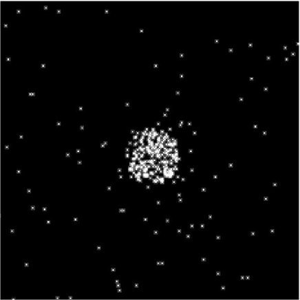
Figure 52.: Chandra image of Mars. Image is 2 arcmin on a side and the Mars disk is 20.3 arcsec in diameter. Courtesy NASA/CXC/MPE/K.Dennerl.

One of the most spectacular Chandra images is the one of the center of our own galaxy (Baganoff et al. 2003) shown in Figure 53. Here we clearly see both point-like discrete sources (over 1000) and diffuse extended emission. This large amount of hot X-ray emitting gas has been heated and chemically enriched by numerous stellar explosions.

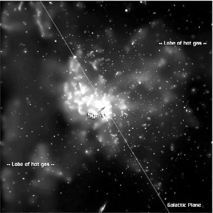
Figure 53.: Chandra image of the Galactic Center. The image is 8.4 arcmin on a side. Courtesy NASA/CXC/MIT/F.K.Baganoff et al.

The final legacy of Chandra may ultimately be led by the spectroscopic data. The energy resolution, enabled by the quality of the optics, is providing new and extremely complex results. The broad bandpass of the grating spectrometers, combined with high resolution, has proven equally important for astrophysical insights in situations where spectral features are not present. For example, the remarkable line-free smoothness of the continuum of the isolated neutron star RXJ 1856-3754 was a spectacular surprise when revealed in detail using a 500 ks observation. This object is the nearest and brightest isolated neutron star candidate (Walter, Wolk & Neuhäuser 1996), and it had been hoped that metal lines formed in its outer atmosphere would provide a direct measurement of gravitational redshift and insights into the equation of state of ultra-dense matter. An early 55 ks exposure lacked the sensitivity to detect weak absorption features (Burwitz et al. 2001), but the 500 ks LETG spectrum placed stringent limits on the strengths of any absorption features (Drake et al. 2002), prompting speculation that its outer layers might lack an atmosphere and reside in a solid state (e.g. Turolla et al. 2004).

Observations with the gratings are not only providing new astrophysical results, they also provide a challenge to atomic physicists. The heart of the LETG+HRC-S bandpass covers the historically relatively uncharted part of the soft X-ray spectrum from 25-70 Å. Prior to Chandra, only a small handful of astrophysical observations had been made at anything approaching high spectral resolution in this range: these were of the solar corona using photographic spectrometers (Widing & Sandlin 1986; Freeman & Jones 1970; Schweizer & Schmidtke 1971; Behring, Cohen, & Feldman 1972; Manson 1972; Acton et al., 1985). In comparison, LETG spectra of similar X-ray sources – the coronae of the solar-like stars $\alpha$ Centuri A (G2 V) and B (K1 V) and of Procyon (Raassen et al. 2002, 2003) – in this range are at the same time both daunting and revealing. The pseudo-continuum of solar coronal emission seen by the 1982 July rocket-borne photographic spectrograph described by Acton et al. (1985) is resolved into a dramatic forest of lines in the LETG spectra. This spectral range contains a superposition of “L-shell” emission of abundant elements such as Mg, Si, S and Ar, providing a challenge to spectroscopists hoping to understand this region in terms of individual atomic transitions. Drake et al. (2004) have shown that current radiative loss models in common usage by X-ray astronomers underestimate the line flux in the 25-70 Å range by factors of up to 5. Laboratory efforts prompted by Chandra spectra, and the need for a better theoretical description of plasma radiative emission in this spectral region, are just beginning to unravel the tangle of lines into their parent ions (e.g. Lepson et al. 2003 and references therein).

Absorption lines also challenge modelers of spectra. “Supersoft” sources and X-ray novae with optically-thick atmospheres at temperatures several $10^{4}$-$10^{5}$ K had been observed many times by ROSAT and BeppoSAX (e.g. Krautter 2002, and references therein). The LETG has revealed that the soft X-ray continuum of these objects hosts a rich array of metal absorption features. Perhaps the best example is the nova V4743 Sgr, which became the brightest X-ray source in the sky at wavelengths above 25 Å ($<0.5$ keV) in early 2003, and was caught using the LETG+HRC-S as a target of opportunity. A preliminary analysis of its spectrum was presented by Ness et al. (2003); the spectrum is shown in Figure 54. While prominent resonance lines of C, N and O can easily be identified, unlike the case of low-density plasmas, the higher density environment of the nova atmosphere in the gravity of its degenerate host can support substantial absorption from excited states that are more difficult to identify. Determining the origin of the multitude of weaker lines “gouging” the continuum will require more complex modeling using realistic model atmospheres. It can be seen from this example how important the unique broad-band sensitivity of the LETG is for disentangling the different parameters describing simple models of these types of source. Coupled with the strong line absorption that modifies the apparent spectrum continuum level is the absorption from intervening material in the circumstellar environment and interstellar medium. The LETG clearly shows this latter attenuation down through two orders of magnitude in flux, out to a wavelength of $\sim 60$ Å (0.2 keV).

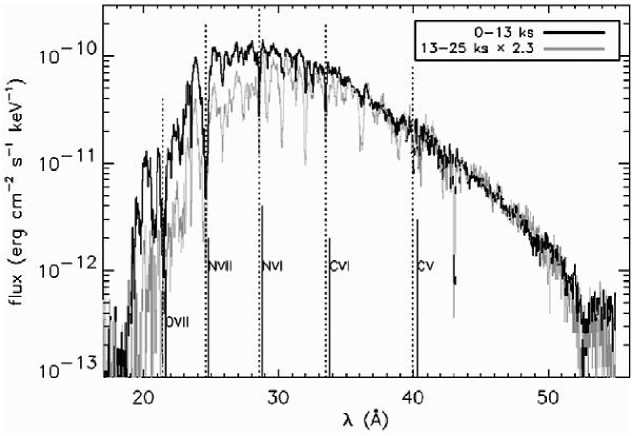
Figure 54.: LETG+HRC-S spectra of the nova V4743 Sgr for two different segments of an observation made on 2003, March 19. Identifications of resonance lines of C, N and O are indicated by vertical lines (solid: rest wavelength; dotted: shifted by -2400 km s-1; from Ness et al. 2003).

High-resolution spectra of Seyfert galaxies are now providing new details about the physical and dynamical properties of material surrounding the active nucleus. For example, the Seyfert 1 active galaxy Mkn 478 was expected to exhibit absorption lines at shorter wavelengths from a warm absorber that has often been seen in the spectra of other Seyfert 1 galaxies, and emission lines at wavelengths of $\sim 100$ Å based on an analysis of EUVE spectra by Hwang & Bowyer (1997). Mkn 478 lies in a direction out of the galaxy that has a particularly low neutral hydrogen column density, and so remains a strong source at these longer wavelengths. Furthermore, for Seyfert-1s, whose signal is dominated by a bright X-ray continuum from the central engine, the partially ionized circum-source material introduces prominent patterns of absorption lines and edges. Figure 55, e.g. shows a LETG/HRC-S spectrum of NGC 5548. This spectrum has dozens of absorption lines (Kaastra et al. 2000). For Seyfert 2’s the strong continuum from the central engine is not seen directly, so the surrounding regions are seen in emission. Figure 56 provides an example of a LETG/HRC observation of the Seyfert 2, NGC 1068 (Brinkman et al. 2002).

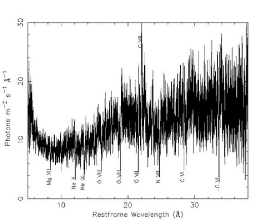
Figure 55.: LETG/HRC spectrum of the Seyfert 1 galaxy NGC 5548 (Kaastra et al. 2000). Several prominent absorption lines from H-like and He-like ions are marked, as is the forbidden line of He-like oxygen.

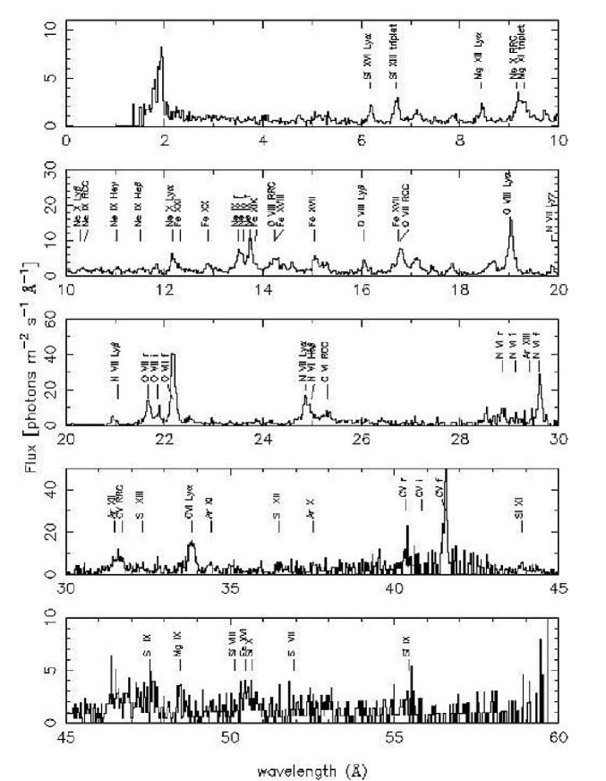
Figure 56.: Emission-line spectrum from the Seyfert 2 galaxy NGC 1068. Kindly provided by A. Kinkhabwala.

One of the more important triumphs of the Observatory has been to use the angular resolution and high sensitivity to perform detailed surveys of extended objects such as globular clusters, galaxies, and clusters of galaxies. Figure 57 shows one of the spectacular Chandra images of globular clusters (Grindlay et al. 2001). A survey of two interacting galaxies is illustrated in Figure 58 where one sees emission from diffuse gas and bright point sources.

Chandra observations of clusters of galaxies frequently exhibit previously undetected structures with characteristic angular scales as small as a few arc seconds. These include ”bubbles” where there is strong radio emission, bow shocks, and cold fronts. These phenomena are illustrated in the sequence of figures, 59-61. Figure 59 of the Perseus cluster (Fabian et al. 2000) is a spectacular example of bubbles produced in regions where there is strong radio emission. Figure 60 shows a bow shock propagating in front of a bullet-like gas cloud just exiting the disrupted cluster core. This observation provided the first clear example of such a shock front (Markevitch et al. 2002). In contrast, Figure 61 of Abell 2142 (Markevitch et al. 2000) shows an example of a shockless cold front.

A major triumph of Chandra (and XMM-Newton) high-resolution spectroscopic observations has been the discovery that that gas in the clusters is typically not cooling to below about 1-2 keV (see for example the discussion in Fabian (2002) which indicates the presence of one (or more) heating mechanisms).

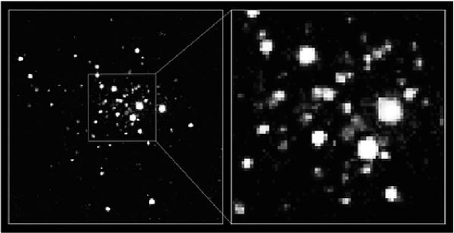
Figure 57.: Chandra ACIS image of the globular cluster 47 Tucanae. The left panel covers the central 2’ x 2.5’. The central 35” x 35” are shown to the right. Courtesy NASA/CfA/J.Grindlay et al.

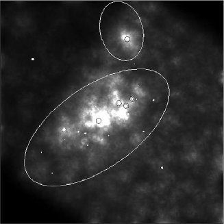
Figure 58.: X-ray image of two interacting galaxies NGC 4490 and 4485. The image is 8-arcmin on a side. Large ovals represent the approximate boundaries of the galaxies (NGC 4490 is the larger of the two). Small circles indicate the brightest X-ray sources. Courtesy Doug Swartz.

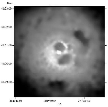
Figure 59.: X-ray core of the Perseus cluster. The image is about 3.5 arcmin on a side. Courtesy NASA/IoA/A. Fabian et al.

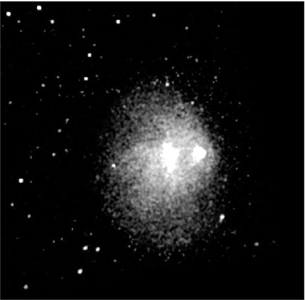
Figure 60.: The Chandra image of the merging, hot galaxy cluster 1E 0657-56. The image is about 9 arcmin on a side. Courtesy NASA/SAO/CXC/M.Markevitch et al.

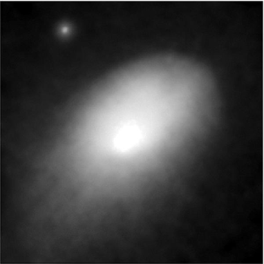
Figure 61.: Chandra Image of the galaxy cluster Abell 2142. The image is 8.4 arcmin on a side. The sharp border to the top right is an example of a cold front. Courtesy NASA/CXC/SAO

Some clusters, such as Abell 2029 shown in Figure 62, do exhibit a smoother relaxed structure. Here we see the thousands of galaxies inside the cocoon of hot, X-ray-emitting gas. Measurement of the temperature and density profiles of the gas, inwards toward the central, dominant galaxy, provides a map of the gravitational potential, and hence the dark matter in the cluster. The observers, Lewis, Buote, and Stocke (2003), showed that the dark matter density increased toward the center in a manner consistent with cold dark matter models.

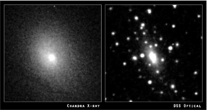
Figure 62.: X-ray (left) and optical (right) images of the galaxy cluster Abell 2029. The images are 4-arcmin on a side. X-ray: NASA/CXC/UCI/A. Lewis et al. Optical: Pal.Obs. DSS

The study of active galaxies is one of the centerpieces of studies with the Observatory. Figure 63 illustrates a recent spectacular result — the first image of a double quasar nucleus (Komossa et al. 2003).

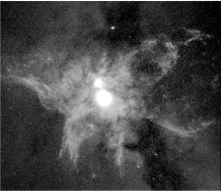
Figure 63.: The Chandra image of NGC 6240, a butterfly-shaped galaxy that is the product of the collision of two smaller galaxies, shows that the central region contains two active galactic nuclei. The image is 0.35 x 0.3 arcmin. Courtesy NASA/CXC/MPE/S. Komossa et al.

Figure 64 illustrates multiwavelength observations of the jets from active galaxies. The Chandra X-ray image (Marshall et al. 2002) shows an irregular, knotty structure similar to that seen at radio and optical (Perlman et al. 2001) wavelengths. However, the knots near the central core are much brighter in X-rays

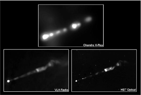
Figure 64.: The X-ray jet emanating from the nucleus of the elliptical galaxy M87 as seen in three wavelength bands. Credits: X-ray: NASA/CXC/MIT/H. Marshall et al. Radio: F. Zhou, F.Owen (NRAO), J.Biretta (STScI) Optical: NASA/STScI/UMBC/E.Perlman et al. (2001).

The jet phenomenon now appears to be ubiquitous in astronomical settings, especially with regards to X-ray emission. One of the most interesting recent Chandra discoveries has been the series of observations of the outer jet of the Vela pulsar (Pavlov et al. 2003), a few of which are illustrated in Figure 65 where we see the jet, always confined to a narrow segment, but moving about at velocities of about 0.3-0.5 c.

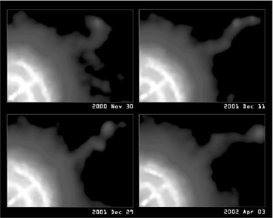
Figure 65.: Four observations of the Vela Pulsar and its outer jet. Each image is 1.6 x 1.2 arcmin Courtesy NASA/CXC/PSU/G. Pavlov et al.

No discussion of data taken with the Observatory is complete without a mention of the deep surveys. These are deep exposures of particular regions of the sky to study the populations of the objects detected, especially the faintest ones. This work is an outgrowth of the study the diffuse X-ray background, the nature of which had been a puzzle for nearly 40 years, although the lack of distortion of the spectrum of the Cosmic Microwave Background placed a strong upper limit to the possibility of a truly diffuse component (Mather et al. 1990). Observations with ROSAT at energies below 2 keV made a major step in resolving a significant fraction (70-80%) into discrete objects (Hasinger et al. 1998). Currently two long exposures have been accomplished with the Chandra X-ray Observatory - the Chandra Deep Field North (Alexander et al. 2003) depicted in Figure 66 with 2-Ms of exposure, and the Chandra deep field south (Giacconi et al. 2001) with 1-Msec. These surveys have extended the study of the background to flux levels more than an order of magnitude fainter than previously in the 0.5-2.0 keV band and have resolved over 90% of the background into a variety of discrete sources. The largest uncertainty in establishing the fraction is now in the knowledge of the total level of the background itself.

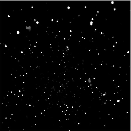
Figure 66.: Two-million-second image of the Chandra Deep Field North. Courtesy NASA/CXC/PSU/D.M. Alexander, F.E. Bauer, W.N. Brandt et al.

8. Conclusions and Acknowledgements

Designed for a minium of three years of operation, the Chandra X-ray Observatory has, in fact, been operating successfully for more than four and one-half years. The instrumentation is well understood and there have been few performance surprises once the Observatory was comissioned for use. The number of new discoveries has been outstanding and the Observatory has more than lived up to its promise. The Observatory has had, and will continue to have, a profound influence on our understanding of the universe, its constituents, and the physical processes that take place within it.

We acknowledge the major contributions to the success of the Observatory and to this paper by the scientists and engineers associated with the instrument teams, the NASA Project at MSFC, the CXC and its Director H. Tananbaum, and the various industrial contractor organizations. TLA, RAC and JJD were supported by NASA contract NAS8-39073. Finally, we acknowlege the tremendous contribution of Leon Van Speybroeck to the Chandra Project and we mourn his passing.

9. WORLD-WIDE WEB SITES

The following lists several Chandra-related sites on the World-Wide Web:

http://chandra.harvard.edu/: Chandra X-ray Center (CXC), operated for NASA by the Smithsonian Astrophysical Observatory.

http://wwwastro.msfc.nasa.gov/xray/axafps.html: Chandra Project Science, at the NASA Marshall Space Flight Center.

http://hea-www.harvard.edu/HRC/: Chandra High-Resolution Camera (HRC) team, at the Smithsonian Astrophysical Observatory (SAO).

http://www.astro.psu.edu/xray/axaf/axaf.html: Advanced CCD Imaging Spectrometer (ACIS) team at the Pennsylvania State University (PSU).

http://acis.mit.edu/: Advanced CCD Imaging Spectrometer (ACIS) team at the Massachusetts Institute of Technology.

http://www.sron.nl/missions/Chandra: Chandra Low-Energy Transmission Grating (LETG) team at the Space Research Institute of the Netherlands.

http://wave.xray.mpe.mpg.de/axaf/: Chandra Low-Energy Transmission Grating (LETG) team at the Max-Planck Institüt für extraterrestrische Physik (MPE).

http://space.mit.edu/HETG/: Chandra High-Energy Transmission Grating (HETG) team, at the Massachusetts Institute of Technology

http://ifkki.kernphysik.uni-kiel.de/soho: EPHIN particle detector.

References

Abell, G. O. & Margon, B. 1979, Nature, 701

Acton, L. W., Bruner, M. E., Brown, W. A., Fawcett, B. C., Schweizer, W., & Speer, R. J. 1985, ApJ, 291, 865

Alexander, D. M., Bauer, F. E., Brandt, W. N., Hornschemeier, A. E., Vignali, C., Garmire, G. P., Schneider, D. P., Chartas, G., & Gallagher, S. C. 2003, AJ, 125, 383

Baganoff, F.K., Maeda, Y., Morris, M., Bautz, M.W., Brandt, W.N., Cui, W., Doty, J.P., Feigelson, E.D., Garmire, G P., Pravdo, S.H., Ricker, G.R.,& Townsley, L.K. 2003, ApJ, 591, 891

Bautz, M. W., Pivovaroff, M., Baganoff, F., Isobe, T., Jones, S. E., Kissel, S. E., LaMarr, B., Manning, H. L., Prigozhin, G. Y., Ricker, G. R., Nousek, J. A., Grant, C. E., Nishikida, K., Scholze, F., Thornagel, R., & Ulm, G. 1998, SPIE, 3444, 210

Behring, W. E., Cohen, L., & Feldman, U. 1972, ApJ, 175, 493

Brandt, W. N., Hornschemeier, A. E., Alexander, D. M., Garmire, G. P., Schneider, D. P., Broos, P. S., Townsley, L. K., Bautz, M. W., Feigelson, E. D., & Griffiths, R. E. 2001, AJ, 122, 1

Brinkman, A. C. et al. 1997, SPIE, 3113, 181

Brinkman, A.C., Kaastra, J. S., van der Meer, R.L.J., Kinkhabwala, A., Behar, E., Paerels, F., Kahn, S.M. & Sako, M. 2002, A&A, 396, 761

Burrows, D. et al. 2000, ApJ, 543, L149.

Burwitz, V., Zavlin, V. E., Neuhäuser, R., Predehl, P., Trümper, J., & Brinkman, A. C. 2001, A&A, 379, L35

Canizares, C.R., Huenemorder, D.P., Davis, D.S., Dewey, D., Flanagam, K.A., Houck, J., Markert, T.H., Marshall, H.L., Schattenburg, M.L., Schulz, N.S., Wise, M., Drake, J.J., & Brickhouse, N.S. 2000, ApJ, bf 539. L41

Dennerl, K. 2002, A&A, 394, 1119.

Dewey, D., Drake, J. J., Edgar, R. J., Michaud, K., & Ratzlaff, P. 1998, SPIE, 3444, 48

Drake, J. J. et al. 2002, ApJ, 572, 996

Drake, J.J., Laming, J.M., Raffauf, E., Kashyap, V. 2004, in prep

Elsner, R. F. et al. 2002, ApJ, 572, 1077

Fabian, A.C., Sanders, J.S., Ettori, S., Taylor, G.B., Allen, S.W., Crawford, C.S., Iwasawa, K., Johnstone, R.M., & Ogle, P.M. 2000, MNRAS, 318, L65.

Fabian, A.C. 2002, ”Cooling Flows in Clusters of Galaxies” in ”Lighthouses of the Universe: The Most Luminous Celestial Objects and Their Use for Cosmology”, Proceedings of the MPA/ESO/, 24.

Freeman, F. F. & Jones, B. B. 1970, Solar Phys., 15, 288

Giacconi, R., Rosati, P., Tozzi, P., Nonino, M., Hasinger, G., Norman, C., Bergeron, J., Borgani, S., Gilli, R., Gilmozzi, R., & Zheng, W. 2001, ApJ, 551, 642

Gladstone, R. et al. 2002, Nature, 415, 1000

Grant, C. E., Bautz, M. W., & Virani, S. N. 2002, in High Energy Universe at Sharp Focus: Chandra Science Symposium, ed. E. M. Schlegel & S. D. Vrtilek, ASP Conf. Ser., 262, 401

Grindlay, J. E., Heinke, C., Edmonds, P. D., & Murray, S. S. 2001, Science, 290, 2292

Hasinger, G. et al. 1998, A&A, 329, 482.

Hellsten, U., Gnedin, N. Y., & Miralda-Escudé, J. 1998, ApJ, 509, 56

Hwang, C-Y, & Bowyer, S. 1997, ApJ, 475, 552

Hwang, U., Holt, S. S., & Petre, R. 2000, ApJ, 537, L119

Juett, A., Schulz, N. S., and Chakrabarty, D., 2004, ApJ, submitted, (astro-ph/0312205)

Kaastra, J.S., Mewe, R., Liedahl, D.A., Komossa, S., & Brinkman, A.C. 2000, Astronomy and Astrophysics, 354, L83.

Kenter, A. T., Kraft, R. P., Meehan, G. R., Murray,S. S., Zombeck, M. V., Donnelly, R. H., Juda, M., Patnaude, D., Pease, D., Fraser, G. W., Pearson,J. F., Lees, J. E., Brunton, A. N., Barbera, M., & Collura, A. 2000, SPIE, 4012, 467

Kraft, R. P., Kenter, A. T., Meehan, R., Murray, S. S., Zombeck, M. V., Donnelly, R. H., Juda, M., Patnaude, D., Pease, D., Fraser, G. W., Pearson, F., Lees, J. E., Brunton, A. N., Barbera, M., & Collura, A., 2000, SPIE, 4012, 493

Komossa, S., Burwitz, V., Hasinger, G., Predehl, P., Kaastra, J. S., & Ikebe, Y. 2003, The Astrophysical Journal, 582, pp. L15-L19.

Krautter, J. 2002, in AIP Conf. Proc. 637, Classical Nova Explosions: Int. Conf. on Classical Nova Explosions, ed. M. Hernanz & J. Jos (Melville: AIP), 345

Kravtsov, A. V., Klypin, A., & Hoffman, Y. 2002, ApJ, 571, 563

Lepson, J. K., Beiersdorfer, P., Behar, E., & Kahn, S. M. 2003, ApJ, 590, 604

Lewis, A.D., Buote, D.A., & Stocke J.T. 2003, Astrophysical Journal, 586, pp. 135-142.

Li, J., Kastner, J. H., Prigozhin, G. Y., & Schulz, N. S. 2003, ApJ, 590, 586

Lopez, L. A., Marshall, H.  L., Canizares C.  R., Kane, J. F., & Schulz, N.  S.  2004, ApJ, submitted

Manson, J. E. 1972, Solar Phys., 27, 107

Margon et al. 1979, ApJ, 230, L41

Markevitch, M., Ponman, T.J., Nulsen, P.E.J., Bautz, M.W., Burke, D.J., David, L.P., Davis, D., Donnelly, R.H., Forman, W.R., Jones, C., & 12 coauthors, 2000, The Astrophysical Journal, 541, pp. 542-549.

Markevitch, M., Gonzalez, A.H., David, L., Vikhlinin, A., Murray, S., Forman, W., Jones, C., Tucker, W. 2002, The Astrophysical Journal, 567, pp. L27-L31.

Markevitch, M., Bautz, M. W., Biller, B., Butt, Y., Edgar, R., Gaetz, T., Garmire, G., Grant, C. E., Green, P., Juda, M., Plucinsky, P. P., Schwartz, D., Smith, R., Vikhlinin, A., Virani, S., Wargelin, B. J., & Wolk, S. 2003, ApJ, 583, 70

Marshall, H.L., Miller, B.P., Davis, D.S., Perlman, E.S., Wise, M., Canizares, C.R., & Harris, D.E. 2002, The Astrophysical Journal, 564, pp. 683-687.22

Marshall, H.  L., Canizares C.  R., & Schulz, N.  S.  2002, ApJ, 564, 941

Marshall, H. L., Edelson, R. A., Vaughan, S,, Malkan, M., O’Brien, P., & Warwick, R. AJ, 125, 459

Marshall, H. L., Tennant, A., Grant, C. E., Hitchcock, A. P., O’Dell, S., & Plucinsky, P. P. 2004, SPIE, bf 5165, 497

Marshall, H. L., Dewey, D., and Ishibashi, K., 2004, SPIE, bf 5165, 457

Mather, J. C. et al. 1990, The Astrophysical Journal, 354, L4.

Mueller-Mellin, R., Kunow, H., Fleissner, V., Pehlke, E., Rode, E., Roeschmann, N., Scharmberg, C., Sierks, H., Rusznyak, P., McKenna-Lawlor, S., Elendt, I., Sequeiros, J., Meziat, D., Sanchez, S., Medina, J., del Peral, L., Witte, M., Marsden, R., & Henrion, J. 1995, Solar Physics,162, 483

Murray, S. S., Austin, G.K., Chappell, J. H., Gomes, J. J., Kenter, A. T., Kraft, R. P., Meehan, G. R., Zombeck, M. V., Fraser, G. W., & Serio, S. 2000, SPIE,4012, 68

Murray, S. S., Slane, P. O., Seward, F. D., Ransom, S. M., & Gaensler, B. M. 2002, ApJ, 568, 226

Ness, J-U, Brickhouse, N, S., Drake, J. J., & Huenemoerder, D. P. 2003, ApJ, bf 598, 1277

Nicastro, F,, Zezas, A., Drake, J., Elvis, M., Fiore, F., Fruscione, A., Marengo, M., Mathur, S., & Bianchi, S. 2002, ApJ, bf 573, 157

Pavlov, G. G., Teter, M. A., Kargaltsev, O., & Sanwal, D. 2003, The Astrophysical Journal, 591, 1157

Perlman, E. S. et al. 2001, The Astrophysical Journal, 561, pp. L51-L54.

Plucinsky, P. P. & Virani, S. N. 2000, Proc SPIE, 2012, 681

Predehl, P. et al. 1997, SPIE, 3113, 172

Prigozhin, G., Kissel, S., Bautz, M., Grant, C., LaMarr, B., Foster, R., & Ricker, G. 2000, SPIE, 4140, 123

Raassen, A. J. J. et al. 2002, A&A, 389, 228

Raassen, A. J. J., Ness, J.-U., Mewe, R., van der Meer, R. L. J., Burwitz, V., & Kaastra, J. S. 2003, A&A, 400, 671

Schweizer, W. & Schmidtke, G. 1971, ApJ, 169, L27

Tennant, A. F., Becker, W., Juda, M., Elsner, R. F., Kolodziejczak, J. J., Murray, S. S., O’Dell, S. L., Paerels, F., Swartz, D. A., Shibazaki, N., & Weisskopf, M. C. 2001 , ApJ,554, 173

Townsley, L. K., Broos, P. S., Nousek, J. A., & Garmire, G. P. 2002, NIM-A, 486, 716

Turolla, R., Zane, S., Drake, J.J., ApJ, in press

Vikhlinin, A. 2002, Reducing ACIS Quiescent Background Using Very Faint Mode, http://cxc.harvard.edu/cal/Links/Acis/acis/Cal_prods/vfbkgrnd/index.html

Walter, F. M., Wolk, S. J., & Neuhaüser, R. 1996, Nature, 379, 233

Weisskopf, M. C., Hester, J. J., Tennant, A. F., Elsner, R. F., Schulz, N. S., Marshall, H. L., Karovska, M., Nichols, J. S., Swartz, D. A., Kolodziejczak, J. J., & O’Dell, S. L. 2000, ApJ, 536, L81

Widing, K. G. & Sandlin, G. D. 1968, ApJ, 152, 545