Power spectrum and correlation function errors: Poisson vs. Gaussian shot noise

Abstract

Poisson distributed shot noise is normally considered in the Gaussian limit in cosmology. However, if the shot noise is large enough and the correlation function/power spectrum conspires, the Gaussian approximation mis-estimates the errors and their covariance significantly. The power spectrum, even for initially Gaussian densities, acquires cross correlations which can be large, while the change in the correlation function error matrix is diagonal except at zero separation. Two and three dimensional power law correlation function and power spectrum examples are given. These corrections appear to have a large effect when applied to galaxy clusters, e.g. for SZ selected galaxy clusters in 2 dimensions. This can increase the error estimates for cosmological parameter estimation and consequently affect survey strategies, as the corrections are minimized for surveys which are deep and narrow rather than wide and shallow. In addition, a rewriting of the error matrix for the power spectrum/correlation function is given which eliminates most of the Bessel function dependence (in two dimensions) and all of it (in three dimensions), which makes the calculation of the error matrix more tractable. This applies even when the shot noise is in the (usual) Gaussian limit.

In cosmology, continuous density fields are used to describe distributions of discrete objects such as galaxy clusters. The actual discrete number counts are taken to be a sampling of this continuous distribution resulting in the appearance of shot noise. Usually the shot noise is taken to have a Gaussian distribution, considered as the large number approximation to an underlying Poisson distribution (Layzer Lay56 (1956), see the textbook by Peebles Pee80 (1980) for a review). The interest here is when the Gaussian approximation for the shot noise breaks down. This paper considers in detail the specific case where the shot noise distribution is in fact Poisson. It is seen that the Poisson nature of the shot noise can produce significant modifications of the Gaussian shot noise error matrix of the correlation function and power spectrum.

The full Poisson power spectrum error matrix was calculated by Meiksin & White MeiWhi99 (1999). In this paper it is angle averaged, compared to usual expressions, and applied to 2 and 3 dimensional power law examples comparable to SZ selected galaxy cluster surveys. The effect on the explicit two dimensional SZ selected galaxy cluster power spectrum is also found and is seen to be large for some realistic survey parameters. These increases to the error matrix have consequences both for cosmological parameter estimates and for designing surveys (the additions only appear if the shot noise is big enough, which can be alleviated by going deeper for an SZ selected survey).

Section one has definitions and the two dimensional angle averaging of the Meiksin & White MeiWhi99 (1999) result. Three dimensions are considered in section two, and section three discusses a rewriting of the error matrix which minimizes the appearance of Bessel functions and their instabilities. This rewriting is also useful for the Gaussian shot noise case. In section four, two and three dimensional power law examples are given, as well as an application to a two dimensional SZ selected galaxy cluster power spectrum. Section five concludes.

The rarity of galaxy clusters and the possible need for Poisson shot noise has been recognized before, e.g. in Lima & Hu LimHu04 (2004) the full Poisson probability function is used to obtain constraints from cluster number counts in conjunction with their scatter.

1 The effect: two dimensions

One can characterize a two dimensional density distribution via its correlation function

$$\langle\hat{\delta}(\vec{r})\hat{\delta}(\vec{r}+\vec{\theta})\rangle$$ (1)

where $\vec{\theta}$ refers to the two dimensional angular separation $(\theta,\phi)$ and the hat denotes an operator. There are actually two averages in the above expression for discrete objects, as the density distribution is treated as a continuous field sampled from the underlying discrete distribution, here the sampling is taken to be Poisson. The first average is over this Poisson sampling, and the second is a sample average, usually assumed to be the same as volume average. The Poisson and sampling average of two density perturbations gives

$$\langle\hat{\delta}(\vec{r})\hat{\delta}(\vec{r}+\vec{\theta})\rangle=w(\vec{\theta})+\frac{\delta_{D}(\vec{\theta})}{\mathcal{N}}$$ (2)

where $\delta_{D}(\vec{\theta})$ is a two-dimensional Dirac delta function, and ${\mathcal{N}}$ is the number density of objects. The angular correlation function $w(\vec{\theta})$ is defined as the probability above random for finding two objects with one in area $\Omega_{1}$ and the other in area $\Omega_{2}$

$$P_{12}={\mathcal{N}}^{2}(1+w(\vec{\theta}))d\Omega_{1}d\Omega_{2}$$ (3)

The operator $\hat{w}$ is usually defined with the shot noise subtracted out:

$$\hat{w}(\vec{\theta})=\hat{\delta}(\vec{r})\hat{\delta}(\vec{r}+\vec{\theta})-\frac{\delta_{D}(\vec{\theta})}{\mathcal{N}}$$ (4)

so that $\langle\hat{w}(\vec{\theta})\rangle=w(\vec{\theta})$.

In practice the measured correlation function will also depend on window functions of the survey $W(\vec{\theta})$,

$$\begin{array}[]{l}\hat{w}(\vec{\theta})=\frac{1}{A(\vec{\theta})}\int d^{2}\theta^{\prime}\int d^{2}\theta^{\prime\prime}W(\vec{\theta}^{\prime})W(\vec{\theta}^{\prime\prime})\hat{\delta}(\vec{\theta}^{\prime})\hat{\delta}(\vec{\theta}^{\prime\prime})\delta_{D}(\vec{\theta}^{\prime}-\vec{\theta}^{\prime\prime}-\vec{\theta})-\frac{\delta_{D}(\vec{\theta})}{\mathcal{N}}\\ A(\vec{\theta})=\int d^{2}\theta^{\prime}d^{2}\theta^{\prime\prime}W(\vec{\theta}^{\prime})W(\vec{\theta}^{\prime\prime})\delta_{D}(\vec{\theta}^{\prime}-\vec{\theta}^{\prime\prime}-\vec{\theta})\;.\end{array}$$ (5)

In the work here the window function is taken to be one inside the region of the survey and zero elsewhere. This simple case illustrates the effect of interest for this paper, however in practice more complicated window functions do arise and can introduce additional subtleties. For more detailed discussion of window functions and errors see Eisenstein & Zaldarriaga EisZal01 (2001).

There is also the Fourier transform of $w(\vec{\theta})$, the power spectrum,

$$P_{2}(\vec{K})=\int d^{2}\theta e^{-i\vec{K}\cdot\vec{\theta}}w(\vec{\theta})\;,$$ (6)

here $\vec{K}=(K,\phi_{k})$. The operator $\hat{P}_{2}(\vec{K})$ also has the shot noise subtracted out (in this case a constant). The operators $\hat{\delta}(\vec{\theta}),\hat{w}(\vec{\theta})$ are dimensionless, while $\hat{P}_{2}(\vec{K})$ is in terms of steradians.

As isotropy is usually assumed in $\vec{K}$ and $\vec{\theta}$ space (this can mean neglecting boundary effects in particular), both $w$ and $P_{2}$ are usually angle averaged:

$$\begin{array}[]{l}w(\theta)=\frac{1}{2\pi}\int d\phi w(\vec{\theta})\\ P_{2}(K)=\frac{1}{2\pi}\int d\phi_{K}P_{2}(\vec{K})\end{array}$$ (7)

The error matrix of the correlation function and power spectrum can be calculated by going back to the definitions of $\hat{w}(\vec{\theta})$ and $\hat{P}(\vec{K})$ in terms of the density. Meiksin & White MeiWhi99 (1999) calculated the Poisson contribution to the error matrix in the power spectrum using counts in cells (Peebles, Pee80 (1980) §36). For Gaussian densities $\hat{\delta}$ the power spectrum error matrix is

$$\begin{array}[]{ll}\langle\hat{P}_{2}(\vec{K})\hat{P}_{2}(\vec{K}^{\prime})\rangle-\langle\hat{P}_{2}(\vec{K})\rangle\langle\hat{P}_{2}(\vec{K}^{\prime})\rangle&=(P_{2}(\vec{K})+\frac{1}{\mathcal{N}})^{2}(\delta_{\vec{K},\vec{K}^{\prime}}+\delta_{\vec{K},-\vec{K}^{\prime}})\\ &\;+\frac{1}{{\mathcal{N}}^{2}\Omega}(P_{2}(|\vec{K}+\vec{K}^{\prime}|)+P_{2}(|\vec{K}-\vec{K}^{\prime}|)+2P_{2}(\vec{K})+2P_{2}(\vec{K}^{\prime}))\\ &\;+\frac{1}{{\mathcal{N}}^{3}\Omega}\\ \end{array}$$ (8)

Here (and later in the text) $\delta_{ab}$ refers to a Kronecker $\delta$ function. If the densities themselves are non-Gaussian, there are additional terms depending upon the three and four point functions,

$$\begin{array}[]{l}\frac{1}{\Omega}T(\vec{K},-\vec{K},\vec{K}^{\prime},-\vec{K}^{\prime})+\frac{1}{{\mathcal{N}}\Omega}[B(\vec{K},-\vec{K},0)+B(0,\vec{K}^{\prime},-\vec{K}^{\prime})\\ +B(\vec{K}+\vec{K}^{\prime},-\vec{K},-\vec{K}^{\prime})+B(\vec{K}-\vec{K}^{\prime},-\vec{K},\vec{K}^{\prime})+B(\vec{K},\vec{K}^{\prime}-\vec{K},-\vec{K}^{\prime})+B(\vec{K},-\vec{K}-\vec{K}^{\prime},\vec{K}^{\prime})]\end{array}$$ (9)

which are Fourier transforms of the spatial four and three point functions $\eta$ and $\zeta$ respectively. These additional terms can be angle averaged (and Fourier transformed) straightforwardly and thus are not shown in the following. They are needed however if the density distribution is non-Gaussian.

There is also an additional term $\frac{1}{{\mathcal{N}}^{3}\Omega}P_{2}(0)$, which may be nonvanishing for some choices of window function. As it is a constant it just modifies

$$\frac{1}{{\mathcal{N}}^{3}\Omega}\rightarrow\frac{1}{{\mathcal{N}}^{3}\Omega}(1+{\mathcal{N}}P_{2}(0))$$ (10)

in the above and in its averages/limits below. The same multiplicative factor ($1+{\mathcal{N}}P_{2}(0)$) (if different from one) occurs in the the last term in the error matrix for the two dimensional correlation function. For three dimensions the last term is instead modified by $(1+{\mathcal{N}}P(0))$. It will not be displayed in the following but can be added in directly if non-zero.

To convert this expression to errors and covariances for the angle averaged correlation function and power spectrum, first take the continuum limit. As

$$\sum_{k}\rightarrow\frac{\Omega}{(2\pi)^{2}}\int d^{2}K\;\;\;\mathrm{and}\;\;\;\sum_{k}\delta_{\vec{K},\vec{K}^{\prime}}=1,$$ (11)

one has the correspondence

$$\delta_{\vec{K},\vec{K}^{\prime}}\rightarrow\frac{(2\pi)^{2}}{\Omega}\delta_{D}({\vec{K}-\vec{K}^{\prime}})\;$$ (12)

and similarly for $\delta_{\vec{K},-\vec{K}^{\prime}}$. Thus the two dimensional power spectrum error matrix is

$$\begin{array}[]{ll}\langle\hat{P}_{2}(\vec{K})\hat{P}_{2}(\vec{K}^{\prime})\rangle-\langle\hat{P}_{2}(\vec{K})\rangle\langle\hat{P}_{2}(\vec{K}^{\prime})\rangle&=(P_{2}(\vec{K})+\frac{1}{\mathcal{N}})^{2}\frac{(2\pi)^{2}}{\Omega}[\delta_{D}({\vec{K}-\vec{K}^{\prime}})+\delta_{D}({\vec{K}+\vec{K}^{\prime}})]\\ &+\frac{1}{{\mathcal{N}}^{2}\Omega}[2P_{2}(\vec{K})+2P_{2}(\vec{K}^{\prime})+P_{2}(|\vec{K}+\vec{K}^{\prime}|)+P_{2}(|\vec{K}-\vec{K}^{\prime}|)]\\ &+\frac{1}{{\mathcal{N}}^{3}\Omega}\end{array}$$ (13)

The Fourier transform of this is the variance of the correlation function $w(\vec{\theta})$:

$$\begin{array}[]{ll}\langle\hat{w}(\vec{\theta})\hat{w}(\vec{\theta}^{\prime})\rangle-\langle\hat{w}(\vec{\theta})\rangle\langle\hat{w}(\vec{\theta}^{\prime})\rangle&=\frac{1}{\Omega}\int d^{2}\theta^{\prime\prime}(w(\vec{\theta}-\vec{\theta}^{\prime}-\vec{\theta}^{\prime\prime})+w(\vec{\theta}+\vec{\theta}^{\prime}-\vec{\theta}^{\prime\prime}))w(\vec{\theta}^{\prime\prime})\\ &+\frac{1}{\Omega{\mathcal{N}}}[2w(\vec{\theta}+\vec{\theta}^{\prime})+2w(\vec{\theta}-\vec{\theta}^{\prime})]\\ &+\frac{1}{\Omega{\mathcal{N}}^{2}}[(\delta_{D}(\vec{\theta}-\vec{\theta}^{\prime})+\delta_{D}(\vec{\theta}+\vec{\theta}^{\prime}))(1+w(\vec{\theta}))\\ &\;\;\;\;\;\;+2w(\vec{\theta})\delta_{D}(\vec{\theta}^{\prime})+2w(\vec{\theta}^{\prime})\delta_{D}(\vec{\theta})]\\ &+\frac{1}{\Omega{\mathcal{N}}^{3}}\delta_{D}(\vec{\theta})\delta_{D}(\vec{\theta}^{\prime})\end{array}$$ (14)

These correlation functions and power spectra are not angle averaged, i.e., they depend upon $\vec{\theta}$ and $\vec{K}$ rather than $\theta,K$. To get the more familiar functions of only $\theta,\theta^{\prime}$ and $K,K^{\prime}$ requires an average over $\phi,\phi^{\prime}$ and $\phi_{k},\phi_{k}^{\prime}$ respectively. (In practice this means ignoring boundary effects, see Eisenstein and Zaldariagga EisZal01 (2001) for discussion.) The correlation function and power spectrum are considered in turn below. The error matrix for each is angle averaged and either binned or discretized. Then each is compared with previous Gaussian expressions in the literature to highlight when and how the additional Poisson-only (or “non-Gaussian”) terms are significant.

For the angular correlation function, angle averaging requires the quantities

$$\frac{1}{2\pi}\int d\phi\delta_{D}(\vec{\theta}-\vec{\theta}^{\prime})=\frac{1}{2\pi}\int d\phi\frac{\delta_{D}(\theta-\theta^{\prime})}{\theta}\delta_{D}(\phi-\phi^{\prime})=\frac{1}{2\pi}\frac{\delta_{D}(\theta-\theta^{\prime})}{\theta}$$ (15)

and

$$\frac{1}{2\pi}\int d\phi\delta_{D}(\vec{\theta}+\vec{\theta}^{\prime})=\frac{1}{2\pi}\int d\phi\frac{\delta_{D}(\theta-\theta^{\prime})}{\theta}\delta_{D}(\phi-\phi^{\prime}\pm\pi)=\frac{1}{2\pi}\frac{\delta_{D}(\theta-\theta^{\prime})}{\theta}$$ (16)

and likewise

$$\frac{1}{2\pi}\int d\phi\delta_{D}(\vec{\theta})=\frac{1}{2\pi\theta}\delta_{D}(\theta)$$ (17)

These relations allow one to get the angle average of all the terms except those containing two $w$’s. For those, go to Fourier space to get

$$\begin{array}[]{ll}\frac{1}{(2\pi)^{2}}\int d\phi d\phi^{\prime}\int d^{2}\vec{\theta}^{\prime\prime}w(\vec{\theta}-\vec{\theta}^{\prime}-\vec{\theta}^{\prime\prime})w(\vec{\theta}^{\prime\prime})&=\ \frac{1}{(2\pi)^{2}}\int d\phi d\phi^{\prime}\int\frac{d^{2}K}{(2\pi)^{2}}e^{i\vec{K}\cdot(\vec{\theta}-\vec{\theta}^{\prime})}P_{2}^{2}(K)\\ &=\int\frac{KdK}{2\pi}J_{0}(K\theta)J_{0}(K\theta^{\prime})P_{2}^{2}(K)\\ \\ \frac{1}{(2\pi)^{2}}\int d\phi d\phi^{\prime}\int d^{2}\vec{\theta}^{\prime\prime}w(\vec{\theta}+\vec{\theta}^{\prime}-\vec{\theta}^{\prime\prime})w(\vec{\theta}^{\prime\prime})&=\int\frac{KdK}{2\pi}J_{0}(K\theta)J_{0}(K\theta^{\prime})P_{2}^{2}(K)\\ \\ \frac{1}{(2\pi)^{2}}\int d\phi d\phi^{\prime}w(\vec{\theta}+\vec{\theta}^{\prime})&=\frac{1}{(2\pi)^{2}}\int d\phi d\phi^{\prime}w(\vec{\theta}-\vec{\theta}^{\prime})\\ &=\int\frac{KdK}{2\pi}J_{0}(K\theta)J_{0}(K\theta^{\prime})P_{2}(K)\\ \end{array}$$ (18)

Putting it all together gives

$$\begin{array}[]{ll}\langle\hat{w}(\theta)\hat{w}(\theta^{\prime})\rangle-&\langle\hat{w}(\theta)\rangle\langle\hat{w}(\theta^{\prime}))\rangle\\ &=\frac{2}{\Omega}\int\frac{KdK}{2\pi}J_{0}(K\theta)J_{0}(K\theta^{\prime})[P_{2}^{2}(K)+\frac{2}{{\mathcal{N}}}P_{2}(K)]+\frac{2}{\Omega{\mathcal{N}}^{2}}\frac{\delta_{D}(\theta-\theta^{\prime})}{2\pi\theta}\\ &\;+\frac{1}{\Omega{\mathcal{N}}^{2}}[2w(\theta)\frac{\delta_{D}(\theta-\theta^{\prime})}{2\pi\theta}+2w(\theta)\frac{\delta_{D}(\theta^{\prime})}{2\pi\theta^{\prime}}+2w(\theta^{\prime})\frac{\delta_{D}(\theta)}{2\pi\theta}]\\ &\;+\frac{1}{\Omega{\mathcal{N}}^{3}}\frac{1}{(2\pi\theta)(2\pi\theta^{\prime})}\delta_{D}(\theta)\delta_{D}(\theta^{\prime})\end{array}$$ (19)

Often the error in $w$ is given in terms of $n_{p}$, the number of pairs. To connect with this expression, binning is needed, i.e. one observes not at just one angle but in a shell of width $\delta\Omega$. This means $w(\theta)$ is not measured at a point but smeared out over a region of size $\Delta\theta$:

$$\hat{w}(\theta)\rightarrow\frac{\int_{-\Delta\theta/2}^{\Delta\theta/2}\hat{w}(\theta+\Delta\theta^{\prime})(\theta+\Delta\theta^{\prime})d(\Delta\theta^{\prime})}{\int_{-\Delta\theta/2}^{\Delta\theta/2}(\theta+\Delta\theta^{\prime})d(\Delta\theta^{\prime})}\equiv\hat{w}_{\Delta\theta}(\theta)\;.$$ (20)

In practice this means that in equation 19 one must replace

$$\begin{array}[]{rl}J_{0}(K\theta)&\rightarrow\frac{1}{\theta\Delta\theta}\int_{-\Delta\theta/2}^{\Delta\theta/2}J_{0}(K(\theta+\Delta\theta^{\prime}))(\theta+\Delta\theta^{\prime})d(\Delta\theta^{\prime})\\ &=\frac{1}{K\theta\Delta\theta}((\theta_{+})J_{1}(K\theta_{+})-(\theta_{-})J_{1}(K\theta_{-}))\\ &\equiv J_{0,\Delta\theta}(K\theta)\\ \theta_{\pm}&=\theta\pm\Delta\theta/2\\ \end{array}$$ (21)

as well as the explicit functions of $w(\theta),w(\theta^{\prime})$ on the right hand side. The continuous $\delta_{D}(\theta-\theta^{\prime})$ functions are effectively replaced by $\delta_{\theta,\theta^{\prime}}/\Delta\theta$. Recognizing $2\pi\theta\Delta\theta=\delta\Omega$ gives

$$\begin{array}[]{ll}\langle\hat{w}_{\Delta\theta}(\theta)\hat{w}_{\Delta\theta}(\theta^{\prime})\rangle\;\;-&\langle\hat{w}_{\Delta\theta}(\theta)\rangle\langle\hat{w}_{\Delta\theta}(\theta^{\prime}))\rangle\\ &=\frac{2}{\Omega}\int\frac{KdK}{2\pi}J_{0,\Delta\theta}(K\theta)J_{0,\Delta\theta}(K\theta^{\prime})[P_{2}^{2}(K)+\frac{2}{\mathcal{N}}P_{2}(K)]+\frac{2}{\Omega{\mathcal{N}}^{2}}\frac{\delta_{\theta,\theta^{\prime}}}{\delta\Omega}\\ &\;+\frac{1}{\Omega{\mathcal{N}}^{2}}[2w_{\Delta\theta}(\theta)\frac{\delta_{\theta,\theta^{\prime}}}{\delta\Omega}+2w_{\Delta\theta}(\theta)\frac{\delta_{\theta^{\prime},0}}{\delta\Omega^{\prime}}+2w_{\Delta\theta}(\theta^{\prime})\frac{\delta_{\theta,0}}{\delta\Omega}]\\ &\;+\frac{1}{\Omega{\mathcal{N}}^{3}}\frac{1}{\delta\Omega\,\delta\Omega^{\prime}}\delta_{\theta,0}\delta_{\theta^{\prime},0}\end{array}$$ (22)

This can be rewritten in terms of the number of pairs, $n_{p}=\frac{1}{2}{\mathcal{N}}^{2}\delta\Omega\Omega$,

$$\begin{array}[]{ll}\langle\hat{w}_{\Delta\theta}(\theta)\hat{w}_{\Delta\theta}(\theta^{\prime})\rangle\;-&\langle\hat{w}_{\Delta\theta}(\theta)\rangle\langle\hat{w}_{\Delta\theta}(\theta^{\prime})\rangle\\ &=\frac{2}{\Omega}\int\frac{KdK}{2\pi}J_{0,\Delta\theta}(K\theta)J_{0,\Delta\theta}(K\theta^{\prime})[P_{2}^{2}(K)+\frac{2}{\mathcal{N}}P_{2}(K)]+\frac{1}{n_{p}}\delta_{\theta,\theta^{\prime}}\\ &\;+\frac{1}{n_{p}}[w_{\Delta\theta}(\theta)\delta_{\theta,\theta^{\prime}}+w_{\Delta\theta}(\theta)\delta_{\theta^{\prime},0}\frac{\delta\Omega}{\delta\Omega^{\prime}}+w_{\Delta\theta}(\theta^{\prime})\delta_{\theta,0}]\\ &\;+\frac{1}{2n_{p}}\frac{\delta_{\theta,\theta^{\prime}}}{{\mathcal{N}}\delta\Omega}\delta_{\theta,0}\end{array}$$ (23)

and $\Omega=4\pi f_{sky}$. This shows the often used $1/n_{p}^{1/2}$ shot noise error estimate in the context of the full correlation function error matrix.

The Poisson rather than Gaussian contributions to the error matrix are the terms on the last two lines above. As these terms are proportional to $1/n_{p}$ they will decrease more quickly with increased binning than the terms involving Bessel functions, i.e. the fractional contribution of the Poisson terms will decrease as the binning increases (assuming the binned $w$ doesn’t increase). The main new contribution is the term proportional to $\delta_{\theta,\theta^{\prime}}w_{\Delta}(\theta)/n_{p}$ which is significant only when $w(\theta)$ is ”large” (relative to one and for large shot noise), i.e. it is most important for small $\theta$. The other terms seem less significant as they only arise when either $\theta$ or $\theta^{\prime}$ are zero.

The terms analogous to the $(1+w)/n_{p}$ were found for the angular correlation function calculated via the Landy-Szalay estimator (Landy & Szalay LanSza93 (1993)) and extended by Bernstein Ber94 (1994) to the case where the correlation function is large enough that the terms depending upon the power are also important.

For the power spectrum, the angle average gives

$$\begin{array}[]{ll}\langle\hat{P}_{2}(K)\hat{P}_{2}(K^{\prime})\rangle-\langle\hat{P}_{2}(K)\rangle\langle\hat{P}_{2}(K^{\prime})\rangle&=\int\frac{d\phi_{k}}{2\pi}\frac{d\phi_{k}}{2\pi}\{(P_{2}(\vec{K})+\frac{1}{\mathcal{N}})^{2}\frac{(2\pi)^{2}}{\Omega}(\delta_{D}({\vec{K}-\vec{K}^{\prime}})+\delta_{D}({\vec{K}+\vec{K}^{\prime}}))\\ &\;+\frac{1}{{\mathcal{N}}^{2}\Omega}[2P_{2}(\vec{K})+2P_{2}(\vec{K}^{\prime})+P_{2}(|\vec{K}+\vec{K}^{\prime}|)+P_{2}(|\vec{K}-\vec{K}^{\prime}|)]\\ &\;+\frac{1}{{\mathcal{N}}^{3}\Omega}\}\\ \\ &=\frac{2\pi}{\Omega}\frac{2}{|K|}\delta_{D}(K-K^{\prime})(P_{2}(K)+\frac{1}{\mathcal{N}})^{2}\\ &\;+\frac{1}{{\mathcal{N}}^{2}\Omega}[2P_{2}(K)+2P_{2}(K^{\prime})+4\pi\int\theta d\theta J_{0}(K\theta)J_{0}(K^{\prime}\theta)w(\theta)]\\ &\;+\frac{1}{{\mathcal{N}}^{3}\Omega}\\ \end{array}$$ (24)

The top line, diagonal in $K,K^{\prime}$, is the usual contribution when the shot noise is Gaussian, rather than Poisson. Here to connect with other formulae in the literature one can make $K$ discrete, in particular $\delta_{D}(K-K^{\prime})\rightarrow\delta_{K,K}/\Delta K=\delta_{K,K^{\prime}}$. Then, replacing $K\rightarrow\ell,\delta_{K,K^{\prime}}=\delta_{\ell,\ell^{\prime}},P_{2}(K)\rightarrow C_{\ell}$ and $\Omega=4\pi f_{sky}$, we can recognize the standard expression for large $\ell$

$$\langle\delta C_{\ell}\delta C_{\ell^{\prime}}\rangle=\delta_{\ell,\ell^{\prime}}\frac{2}{(2\ell+1)f_{sky}}(C_{\ell}+\frac{1}{\mathcal{N}})^{2}\sim\delta_{\ell,\ell^{\prime}}\frac{1}{f_{sky}}\frac{1}{\ell}(C_{\ell}+\frac{1}{\mathcal{N}})^{2}$$ (25)

The completely binned expression is found by replacing $P_{2}(K)$ by

$$P_{2}(K)\rightarrow\frac{1}{K\Delta K}\int_{-\Delta K/2}^{\Delta K/2}d(\Delta\tilde{K})(K+\Delta\tilde{K})P_{2}(K+\Delta\tilde{K})$$ (26)

and likewise for $P_{2}(K^{\prime})$ on the left hand side of eqn. 24 and averaging the functions of $K,K^{\prime}$ on the right hand side analogously.

The Poisson terms are non-diagonal and introduce cross correlations in the power spectrum. The cross correlation grows with the separation $K-K_{ref}$ up to some limiting value, ignoring binning one has

$$\frac{\langle P_{2}(K_{ref})P_{2}(K)\rangle}{\sqrt{\langle P_{2}(K_{ref})P_{2}(K_{ref})\rangle\langle P_{2}(K)P_{2}(K)\rangle}}\rightarrow_{K{\rm large}}{\mathcal{N}}^{3/2}\frac{2P_{2}(K_{ref})/{\mathcal{N}}^{2}+1/{\mathcal{N}}^{3}}{\sqrt{\langle P_{2}(K_{ref})P_{2}(K_{ref})\rangle}}\;;$$ (27)

This additional covariance makes the power spectrum errors correlated even if the density distribution was originally Gaussian. The size of this cross correlation is shown in examples in section four, it can be large.

The errors have both Gaussian and non-Gaussian contributions, the non-Gaussian terms become comparable to the Gaussian terms when $2\pi{\mathcal{N}}^{2}P_{2}(K)/K\leq 1$ and $P_{2}(K)K\geq 2\pi$, when there is no binning. In contrast to the correlation function case, increasing the binning increases the importance of the additional non-Gaussian terms as binning roughly divides the first (i.e. Gaussian) term by the bin size relative to the others. In section four it is shown that for ${\mathcal{N}}$, $P_{2}(K)$ and $K$ of interest for SZ selected galaxy cluster surveys the Poisson contribution to the errors can be relatively large.

2 Three dimensions

In three dimensions the correlation function $\xi(r)$ and power spectrum $P(k)$ are related via

$$\begin{array}[]{l}P(\vec{k})=\int d^{3}re^{-i\vec{k}\cdot\vec{r}}\xi(\vec{r})\\ \xi(\vec{r})=\frac{1}{(2\pi)^{3}}\int d^{3}ke^{i\vec{k}\cdot\vec{r}}P(\vec{k})\\ \end{array}$$ (28)

To angle average these we again need to assume isotropy and that boundary effects aren’t important. In three dimensions, ${\mathcal{N}}$ denotes the number density per $(h^{-1}{\rm Mpc})^{3}$. The three dimensional continuum limit of the Meiksin & White MeiWhi99 (1999) error matrix calculation is

$$\begin{array}[]{ll}\langle\hat{P}(\vec{K})\hat{P}(\vec{K}^{\prime})\rangle-\langle\hat{P}(\vec{K})\rangle\langle\hat{P}(\vec{K}^{\prime})\rangle&=\langle\hat{P}(\vec{K})\hat{P}(\vec{K}^{\prime})\rangle-P(\vec{K})P(\vec{K}^{\prime})\\ &=\frac{(2\pi)^{3}}{V}(P(\vec{K})+\frac{1}{\mathcal{N}})^{2}(\delta_{D}(\vec{K}-\vec{K}^{\prime})+\delta_{D}(\vec{K}+\vec{K}^{\prime}))\\ &+\frac{1}{{\mathcal{N}}^{2}V}[P(|\vec{K}+\vec{K}^{\prime}|)+P(|\vec{K}-\vec{K}^{\prime}|)+2P(\vec{K})+2P(\vec{K}^{\prime})]\\ &+\frac{1}{{\mathcal{N}}^{3}V}\\ \end{array}$$ (29)

Fourier transforming to get the correlation function, angle averaging via

$$\frac{1}{4\pi}\int d\Omega\frac{1}{4\pi}\int d\Omega^{\prime}$$ (30)

and using

$$\delta_{D}(\vec{r}-\vec{r}^{\prime})=\frac{\delta_{D}(r-r^{\prime})}{r^{2}}\delta_{D}(\Omega-\Omega^{\prime})$$ (31)

gives

$$\begin{array}[]{ll}\langle\hat{\xi}(r)\hat{\xi}(r^{\prime})\rangle-\langle\hat{\xi}(r)\rangle\langle\hat{\xi}(r^{\prime})\rangle&=\frac{1}{V\pi^{2}}\int k^{2}dk(\frac{\sin(kr)}{kr})(\frac{\sin(kr^{\prime})}{kr^{\prime}})P(k)^{2}\\ &\;+\frac{2}{V{\mathcal{N}}\pi^{2}}\int k^{2}dk(\frac{\sin(kr)}{kr})(\frac{\sin(kr^{\prime})}{kr^{\prime}})P(k)+\frac{1}{V{\mathcal{N}}^{2}}\frac{2}{4\pi r^{2}}\delta_{D}(r-r^{\prime})\\ &\;+\frac{1}{V{\mathcal{N}}^{2}}[\frac{2}{4\pi r^{2}}\delta_{D}(r-r^{\prime})\xi(r)+2\xi(r)\frac{1}{4\pi r^{{}^{\prime}2}}\delta_{D}(r^{\prime})+2\xi(r^{\prime})\frac{1}{4\pi r^{{}^{\prime}2}}\delta_{D}(r)]\\ &\;+\frac{1}{V{\mathcal{N}}^{3}}\frac{1}{4\pi r^{2}}\delta_{D}(r)\frac{1}{4\pi r^{{}^{\prime}2}}\delta_{D}(r^{\prime})\}\\ \end{array}$$ (32)

The additional non-Gaussian terms are the same as in the two dimensional case, i.e. diagonal and proportional to $\xi(r)/n_{p}$ when binning is included plus contributions if either $r$ or $r^{\prime}$ are zero. In this case $n_{p}={\mathcal{N}}^{2}V4\pi r^{2}\Delta r/2$.

For the power spectrum, the angle average gives

$$\begin{array}[]{ll}\langle(\hat{P}(K)-P(K))(\hat{P}(K^{\prime})-P(K^{\prime}))\rangle&=\frac{4\pi^{2}}{|K|^{2}V}(P(K)+\frac{1}{\mathcal{N}})^{2}\delta_{D}(K-K^{\prime})\\ &\;+\frac{2}{{\mathcal{N}}^{2}V}(P(K)+P(K^{\prime})+4\pi\int r^{2}dr\frac{\sin Kr}{Kr}\frac{\sin K^{\prime}r}{K^{\prime}r}\xi(r))\\ &\;+\frac{1}{{\mathcal{N}}^{3}V}\\ \end{array}$$ (33)

The error matrix for the power spectrum also has the same structure as in two dimensions: the Poisson terms introduce correlations between different values of $K$, and analogously, the non-Gaussian nature of the shot noise will start to become important for the errors if $4\pi^{2}\frac{{\mathcal{N}}^{2}P(k)}{|K|^{2}}\leq 1$ and $|K|^{2}P(K)>4\pi^{2}$. With binning the first (Gaussian) term gets a factor of one over the size of the bin, in three dimensions this coefficient is likely to be less than one.

3 Errors without Bessel functions

The error matrices for the power spectrum and the correlation function above each depend on both the correlation function and the power spectrum. This is less than ideal because going between power spectra and correlation functions involves integrals over Bessel functions $J_{0}$ in two dimensions and spherical Bessel functions $j_{0}(x)=\sin(x)/x$ in three dimensions. Integrals against these Bessel functions do not converge quickly; with real data and thus perhaps incomplete coverage in real or momentum space the results may not be very accurate. If one wished to sidestep this problem by using the measured correlation functions and power spectra together to calculate the errors for either, one would be combining quantities which have very different estimators and thus systematics.

However, as the correlation function and power spectrum are Fourier transforms of each other, one can instead substitute the definitions until one has errors in the correlation functions only in terms of correlation functions or similarly for the power spectrum, integrated against an integral of a combination of regular or spherical Bessel functions. This integral of (spherical) Bessel functions will not depend on the power spectrum or correlation function and can be calculated separately. For three Bessel functions and three and four spherical Bessel functions the exact value of this integral is simple and can be used directly, for four Bessel functions the result involves an elliptic integral.

This rewriting is only valid when the power spectrum or correlation function(s) is/are well behaved enough that the order of integration can be changed. In these cases it can provide an immense simplification of the calculation. The integral for three (spherical) Bessel functions in two (three) dimensions is explicitly cut off, and the functions involved are not as oscillatory as Bessel functions in all cases where a simple rewriting was found, providing more numerical stability for calculating the errors. Unless one uses the elliptic integral expression for the four Bessel functions, this rewriting doesn’t completely eliminate the Bessel functions needed to calculate the error matrix for (even a well behaved) $w(\theta)$. The substitution and integrals are done below, first for the two dimensional correlation function and power spectrum and then their counterparts in three dimensions.

For the two dimensional correlation function, the error matrix for $w$ is given by equation 19. If the rise of $w(\theta)$ is shallow enough at the origin, one can rewrite the term with just one $P_{2}(K)$ via

$$\begin{array}[]{l}\int\frac{KdK}{2\pi}J_{0}(K\theta)J_{0}(K\theta^{\prime})P_{2}(K)\\ =\int\theta^{\prime\prime}d\theta^{\prime\prime}w(\theta^{\prime\prime})\int KdKJ_{0}(K\theta)J_{0}(K\theta^{\prime})J_{0}(K\theta^{\prime\prime})\\ =\int\theta^{\prime\prime}d\theta^{\prime\prime}w(\theta^{\prime\prime})f(\theta,\theta^{\prime},\theta^{\prime\prime})\\ \end{array}$$ (34)

where $f(\theta,\theta^{\prime},\theta^{\prime\prime})$ is known in closed form (Jackson & Maximon JacMax72 (1972)), i.e.

$$f(\theta,\theta^{\prime},\theta^{\prime\prime})=\frac{\Delta(\theta,\theta^{\prime},\theta^{\prime\prime})}{2\pi A(\theta,\theta^{\prime},\theta^{\prime\prime})}\;.$$ (35)

Here

$$\begin{array}[]{ll}\Delta(\theta,\theta^{\prime},\theta^{\prime\prime})&=\left(\begin{array}[]{ll}1&{\rm if}\;\theta+\theta^{\prime}>\theta^{\prime\prime},\theta+\theta^{\prime\prime}>\theta^{\prime},\theta^{\prime}+\theta^{\prime\prime}>\theta\\ \frac{1}{2}&{\rm if}\;\theta+\theta^{\prime}=\theta^{\prime\prime}\;{\rm or}\;\theta+\theta^{\prime\prime}=\theta^{\prime}\;{\rm or}\;\theta^{\prime}+\theta^{\prime\prime}=\theta\\ 0&{\rm otherwise}\\ \end{array}\right.\\ A(\theta,\theta^{\prime},\theta^{\prime\prime})&=\frac{1}{2}\sqrt{(\theta+\theta^{\prime}+\theta^{\prime\prime})(-\theta+\theta^{\prime}+\theta^{\prime\prime})(\theta-\theta^{\prime}+\theta^{\prime\prime})(\theta+\theta^{\prime}-\theta^{\prime\prime})}\end{array}$$ (36)

Geometrically, $A$ is the area of the triangle formed with 3 lines of length $\theta,\theta^{\prime},\theta^{\prime\prime}$; $\Delta$ is 1 if the triangle is non-degenerate, 1/2 if it is degenerate and zero if no triangle is formed. In particular, $\Delta$ will cut off the integral over $\theta^{\prime\prime}$ for $\theta^{\prime\prime}>\theta+\theta^{\prime}$. For any two sides equalling the third $f$ diverges, but in the integral it is an integrable divergence; integrating by parts gives a finite result.

Unfortunately a simple expression (without elliptic integrals) for

$$\int dk\,kJ_{0}(k\theta)J_{0}(k\theta^{\prime})J_{0}(k\theta^{\prime\prime})J_{0}(k\theta^{\prime\prime\prime})$$ (37)

was not found, so there is still some explicit $P_{2}(K)$ dependence in $\langle ww\rangle$.

In terms of $f(\theta,\theta^{\prime},\theta^{\prime\prime})$:

$$\begin{array}[]{ll}\langle\hat{w}(\theta)\hat{w}(\theta^{\prime})\rangle-\langle\hat{w}(\theta)\rangle\langle\hat{w}(\theta^{\prime}))\rangle&=\frac{2}{\Omega}\int\frac{KdK}{2\pi}J_{0}(K\theta)J_{0}(K\theta^{\prime})P_{2}^{2}(K)+\frac{4}{\Omega{\mathcal{N}}}\int d\theta^{\prime\prime}\theta^{\prime\prime}w(\theta^{\prime\prime})f(\theta,\theta^{\prime},\theta^{\prime\prime})\\ &+\frac{1}{\Omega{\mathcal{N}}^{2}}[2(1+w(\theta))\frac{\delta_{D}(\theta-\theta^{\prime})}{2\pi\theta}+2w(\theta)\frac{\delta_{D}(\theta^{\prime})}{2\pi\theta^{\prime}}+2w(\theta^{\prime})\frac{\delta_{D}(\theta)}{2\pi\theta}]\\ &+\frac{1}{\Omega{\mathcal{N}}^{3}}\frac{1}{(2\pi\theta)(2\pi\theta^{\prime})}\delta_{D}(\theta)\delta_{D}(\theta^{\prime})\end{array}$$ (38)

For the angular power spectrum, there is no quadratic term in $w$ so if $P_{2}(K)$ is not too singular at the origin, its error matrix can be rewritten completely in terms of $P_{2}(K)$ itself:

$$\begin{array}[]{ll}\langle\hat{P}_{2}(K)\hat{P}_{2}(K^{\prime})\rangle-\langle\hat{P}_{2}(K)\rangle\langle\hat{P}_{2}(K^{\prime})\rangle&=\frac{2\pi}{\Omega}\frac{2}{|K|}\delta_{D}(K-K^{\prime})(P_{2}(K)+\frac{1}{\mathcal{N}})^{2}\\ &+\frac{1}{{\mathcal{N}}^{2}\Omega}(2P_{2}(K)+2P_{2}(K^{\prime}))+\frac{2}{{\mathcal{N}}^{2}\Omega}\int K^{\prime\prime}\,dK^{\prime\prime}f(K,K^{\prime},K^{\prime\prime})P_{2}(K^{\prime\prime})\\ &+\frac{1}{{\mathcal{N}}^{3}\Omega}\\ \end{array}$$ (39)

where $f(K,K^{\prime},K^{\prime\prime})$ is the same function as in equation 35, with the replacement $\theta\to K$ etc. Smoothing is done straightforwardly.

For three dimensions all the integrals over spherical Bessel functions can be done exactly, and the applicability of this substitution is limited only by the requirement of sufficient falloff of the power spectrum and the correlation function at the origin. In terms of these integrals the error matrices from section three become

$$\begin{array}[]{ll}\langle\hat{\xi}(r)\hat{\xi}(r^{\prime})\rangle-\langle\hat{\xi}(r)\rangle\langle\hat{\xi}(r^{\prime})\rangle&=\frac{16}{V}\int r^{{}^{\prime\prime}2}dr^{\prime\prime}r^{{}^{\prime\prime\prime}2}dr^{\prime\prime\prime}\xi(r^{\prime\prime})\xi(r^{\prime\prime\prime})g_{3}(r,r^{\prime},r^{\prime\prime},r^{\prime\prime\prime})\\ &+\frac{8}{V{\mathcal{N}}\pi}\int r^{{}^{\prime\prime}2}dr^{\prime\prime}\xi(r^{\prime\prime})f_{3}(r,r^{\prime},r^{\prime\prime})\\ &+\frac{1}{V{\mathcal{N}}^{2}}[\frac{2}{4\pi r^{2}}\delta_{D}(r-r^{\prime})(1+\xi(r))+2\xi(r)\frac{1}{4\pi r^{{}^{\prime}2}}\delta_{D}(r^{\prime})+2\xi(r^{\prime})\frac{1}{4\pi r^{{}^{\prime}2}}\delta_{D}(r)]\\ &+\frac{1}{V{\mathcal{N}}^{3}}\frac{1}{4\pi r^{2}}\delta_{D}(r)\frac{1}{4\pi r^{{}^{\prime}2}}\delta_{D}(r^{\prime})\}\\ \end{array}$$ (40)

for the correlation function and

$$\begin{array}[]{ll}\langle(\hat{P}(K)-P(K))(\hat{P}(K^{\prime})-P(K^{\prime}))\rangle&=\frac{4\pi^{2}}{|K|^{2}V}(P(K)+\frac{1}{\mathcal{N}})^{2}\delta_{D}(K-K^{\prime})\\ &\;+\frac{2}{{\mathcal{N}}^{2}V}(P(K)+P(K^{\prime})+\frac{2}{\pi}\int_{0}^{\infty}dK^{\prime\prime}K^{{}^{\prime\prime}2}P(K^{\prime\prime})f_{3}(K,K^{\prime},K^{\prime\prime}))\\ &\;+\frac{1}{{\mathcal{N}}^{3}V}\\ \end{array}$$ (41)

for the power spectrum.

Here

$$\begin{array}[]{l}f_{3}(r,r^{\prime},r^{\prime\prime})=\int_{0}^{\infty}k^{2}dk\frac{\sin(kr)}{kr}\frac{\sin(kr^{\prime})}{kr^{\prime}}\frac{\sin(kr^{\prime\prime})}{kr^{\prime\prime}}\\ \;\;\;=\frac{\pi}{8}(-\rm sgn(r-r^{\prime}-r^{\prime\prime})+\rm sgn(r+r^{\prime}-r^{\prime\prime})+\rm sgn(r-r^{\prime}+r^{\prime\prime})-\rm sgn(r+r^{\prime}+r^{\prime\prime}))\\ \;\;\;=\frac{\pi}{8}(-\rm sgn(r-r^{\prime}-r^{\prime\prime})+\rm sgn(r+r^{\prime}-r^{\prime\prime})+\rm sgn(r-r^{\prime}+r^{\prime\prime})-1)\\ \\ g_{3}(r,r^{\prime},r^{\prime\prime},r^{\prime\prime\prime})=\int_{0}^{\infty}k^{2}dk\frac{\sin(kr)}{kr}\frac{\sin(kr^{\prime})}{kr^{\prime}}\frac{\sin(kr^{\prime\prime})}{kr^{\prime\prime}}\frac{\sin(kr^{\prime\prime\prime})}{kr^{\prime\prime\prime}}\\ \;\;\;\;=\frac{\pi}{16}\{|r-r^{\prime}-r^{\prime\prime}-r^{\prime\prime\prime}|-|r+r^{\prime}-r^{\prime\prime}-r^{\prime\prime\prime}|-|r-r^{\prime}+r^{\prime\prime}-r^{\prime\prime\prime}|+|r+r^{\prime}+r^{\prime\prime}-r^{\prime\prime\prime}|\\ \;\;\;\;-|r-r^{\prime}-r^{\prime\prime}+r^{\prime\prime\prime}|+|r+r^{\prime}-r^{\prime\prime}+r^{\prime\prime\prime}|+|r-r^{\prime}+r^{\prime\prime}+r^{\prime\prime\prime}|-(r+r^{\prime}+r^{\prime\prime}+r^{\prime\prime\prime})\}\\ \end{array}$$ (42)

As mentioned above, these rewritings have many advantages besides getting rid of the instabilities due to oscillations of the (spherical) Bessel functions. The functions $f$ and $f_{3}$ cut off the integrals for large argument: i.e. in two dimensions $f(\theta,\theta^{\prime},\theta^{\prime\prime})$ is zero when $\theta^{\prime\prime}>\theta+\theta^{\prime}$ and in three dimensions, e.g., for $K=K^{\prime}$ in the power spectrum, the term with $f_{3}$ becomes

$$\frac{2}{\pi}\int_{0}^{\infty}dK^{\prime\prime}K^{{}^{\prime\prime}2}P(K^{\prime\prime})\frac{\pi}{8}(1+\rm sgn(2K-K^{\prime\prime}))=\frac{1}{2}\int_{0}^{2K}dK^{\prime\prime}K^{{}^{\prime\prime}2}P(K^{\prime\prime})$$ (43)

with an analogue that can be seen by inspection for $K\neq K^{\prime}$. These cutoffs reduce the dependence on the asymptotic values of the power spectrum or the correlation function. The function $g_{3}(r,r^{\prime},r",r^{\prime\prime\prime})$ also goes to zero as $r^{\prime\prime}$ or $r^{\prime\prime\prime}$ goes to infinity, but as both parameters are varying some care must be taken in the joint limits.

4 Examples

In this section the full Poisson error matrices given above are calculated for a power law power spectrum in two and three dimensions and compared to the usual Gaussian error matrix. In addition, the effects on the angular power spectrum errors for SZ selected galaxy clusters are shown. For these examples the corrections are significant except for the two dimensional correlation function. The signal is taken to be Gaussian; if not, the three and four point functions mentioned earlier would need to be included.

Starting with two dimensions, consider a power law power spectrum

$$P_{2}(K)=A_{k}k^{n}$$ (44)

with corresponding correlation function $w(\theta)=A_{\theta}\theta^{-n-2}$. For the error matrix to converge, $-1<n<-1/2$, take $n=-0.9$ for illustration, $A_{k}=5.0\times 10^{-4}$ and thus $A_{\theta}=7.0\times 10^{-5}$. This is a rough fit to the power spectrum for SZ selected clusters for $Y_{min}=1.7\times 10^{-5}$ such as might be seen with APEX. We vary the number density of objects per steradian, ${\mathcal{N}}$ and the binnings $\Delta\theta$ and $\Delta K$. The objects are taken to have a Gaussian distribution, and $f_{sky}=1/4\pi$, i.e. one steradian. The terms in the error matrix all increase by a multiplicative factor $1/f_{sky}$ for other values of $f_{sky}$.

The true cluster case differs from this in three ways: $P_{2}(K)$ and $w(\theta)$ are not true power laws, the number density is fixed (for clusters with the above $Y_{min}$, ${\mathcal{N}}\sim 33000$ is expected) and the cluster distribution is not expected to be Gaussian to arbitrarily small scales. The cluster power spectrum and number densities for an experiment such as APEX or Planck are shown later on, however the signal is still taken to be Gaussian and $f_{sky}$ remains $1/4\pi$.

For terminology, error means the square root of the diagonal (i.e. $K=K^{\prime}$ for power) term in the error matrix. The “shot noise” error means the term $n_{p}^{-1/2}$ in the error of $w(\theta)$ and the term proportional to $\frac{1}{|K|^{1/2}{\mathcal{N}}}$ in the error of $P_{2}(K)$. The “Gaussian error” refers to the terms which arise when the shot noise is considered to be Gaussian rather than Poisson, i.e. the first line on the right in equations 23 and 24 and their three dimensional generalizations. The “non-Gaussian” error or “Poisson” error is everything else in the error. Similarly, “non-Gaussian” and “Poisson” refer to the analogous terms in the rest of the error matrix.

Figure one shows the effects for the correlation function. The delta function errors which only appear at the origin have not been included.

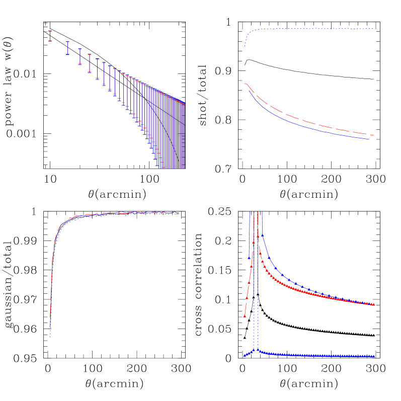
Figure 1: Upper left: Shot noise, Gaussian and full errors for $w(\theta)$, with ${\mathcal{N}}=35000$, 5 arcmin smoothing, and $f_{sky}=1/4\pi$. The curved line is the angular power spectrum for SZ selected galaxy clusters with $Y_{min}=1.7\times 10^{-5}$ as mentioned in the text. Upper right: shot noise as fraction of total correlation function error for 5 arcmin smoothing and ${\mathcal{N}}$ = 5000, 35000 and 65000 objects per steradian, and then for 15 arcmin smoothing and ${\mathcal{N}=35000}$, top to bottom. Lower left: the ratio of using only errors calculated with the Gaussian approximation for Poisson noise, divided by the full errors, for all four cases. Lower right: The cross correlation, $\langle w(\theta)w(30^{\prime})\rangle/\sqrt{\langle w(30^{\prime})w(30^{\prime})\rangle/\langle w(\theta)w(\theta)\rangle}$ as a function of angle for the angular correlation function for 5 arcmin smoothing and three different cases of object numbers (5000,35000,65000 from bottom to top) and for 15 arcmin smoothing and ${\mathcal{N}}=35000$ (very top).

At top left is the angular correlation function for ${\mathcal{N}}=35000$ with shot, Gaussian and full error bars. The smoothing is 5 arcmin, i.e. the spacing between the error bars. The curved line is the correlation function for the analogous SZ cluster sample with $Y_{min}=1.7\times 10^{-5}$. Figure 1 upper right and lower left show the fraction of shot noise alone to the total error and Gaussian error to total error as a function of changing ${\mathcal{N}}$ respectively. As can be seen, although the shot noise is a significant source of the error, using only the shot noise underestimates the error by some noticeable fraction unless the shot noise is extremely large (${\mathcal{N}}=5000$ here). The non-Gaussian terms in the error are an equally small proportion of the total error for all three values of ${\mathcal{N}}$ considered here. The dominance of the shot noise in the error means that the cross correlation decreases as the shot noise increases, as can be seen in the lower right hand panel for the three different ${\mathcal{N}}$ values and also the case with binning of 15 arcmin rather than 5 arcmin. As mentioned earlier, increased binning reduces the relative contribution of the shot noise error to the total error and increases the cross correlation for a fixed number density.

For the angular power spectrum, the corresponding quantities are shown in figure two. Here smoothing is in equal intervals in log $K$. The curved line is the expected angular power spectrum for the SZ selected cluster survey mentioned above. The non-Gaussian contribution to the error matrix is very important!

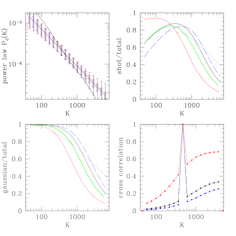
Figure 2: Upper left: angular power spectrum with full errors, Gaussian errors, and only shot noise errors, largest to smallest error bars respectively. Error bars are slightly offset. Upper right: shot noise only as fraction of total error for 20 K bins smoothed in log K and ${\mathcal{N}}$ = 5000, 35000 and 65000, and for 10 k bins and 20 equal $K$ rather than log $K$ bins with ${\mathcal{N}}$ = 35000. Lower left: Gaussian errors divided by the full errors, for all five cases. The lowest line (at far right of each figure) is for ${\mathcal{N}}=5000$, the second lowest is that for using 10 bins, and then the next two going up are ${\mathcal{N}}=35000,65000$. The highest (dotted) line is for 20 equal bins in $K$ rather than log $K$. Lower right: the cross correlation for the power spectrum, $\langle P_{2}(469)P_{2}(K)\rangle/\sqrt{\langle P_{2}(469)P_{2}(469)\rangle/\langle P_{2}(K)P_{2}(K)\rangle}$ as a function of $K$ for 20 log $K$ bins and three different choices of object numbers (5000,35000,65000 from top to bottom).

At upper left are the shot only, Gaussian and full errors for ${\mathcal{N}}=35000$, the curved line is the reference SZ selected galaxy cluster angular power spectrum mentioned earlier. Upper right and lower left are the ratios of the shot noise only and Gaussian errors only to the total error as a function of $K$, and lower right is the cross correlation. The cross correlation is large and is entirely induced by the Poisson nature of the shot noise given our assumptions that $\eta$ and $\zeta$ are zero. The effect of the binning, as $K>1$, is to make the Gaussian contribution even a smaller fraction of the total error matrix. Binning in equal size bins in $K$ rather than log $K$ increases the Gaussian contribution to the error at larger $K$ (as the bins are smaller at large $K$ in this case), however the Poisson nature of the shot noise still makes the ratio of the Gaussian to full error small. The case for ${\mathcal{N}}=35000$ and 20 equal bins in $K$ rather than log $K$ is shown to illustrate this. The change induced by using the Poisson rather than Gaussian error matrix is large, for example, for $K=2000$ and ${\mathcal{N}}=35000$ the error bar increases by close to a factor of two, and the cross correlation with $K=469$ is $\sim 0.5$ rather than zero.

The case of SZ selected galaxy clusters with specific modeling and cosmological assumptions can be done analogously: i.e. with the Evrard mass function (Evrard et al Evretal02 (2002)), Sheth-Tormen bias (Sheth & Tormen SheTor99 (1999)), Eisenstein-Hu (Eisenstein & Hu EisHu97 (1997)) transfer function, $T_{*}^{SZ}=1.2keV$ and $\sigma_{8}=0.9$, $\Omega_{m}=0.3$. Details of the calculation to get this curve and assumptions can be found in Cohn & Kadota CohKad04 (2005). The error matrix for $Y_{min}=1.7\times 10^{-5}$ is extremely close to those for the ${\mathcal{N}}=35000$ example in figure one. Figure three shows the fraction of total errors given by the Gaussian approximation, and the cross correlation for $Y_{min}=1.7\times 10^{-5},3.4\times 10^{-5},1.0\times 10^{-4}$ (with ${\mathcal{N}}$ determined by $Y_{min}$ and the other parameters mentioned before). A $Y_{min}=3.4\times 10^{-5}$ might arise if the survey was wider and shallower, and $Y_{min}=10^{-4}$ is a rough estimate of the errors for Planck (even smaller effective $Y_{min}$ might arise once cluster finding is applied (Geisbusch et al GeiKneHob04 (2004), for example).

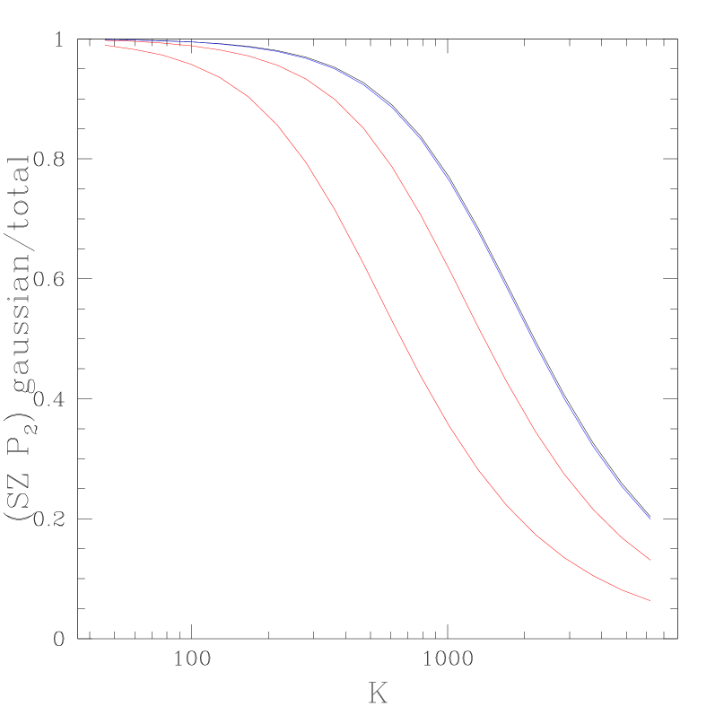
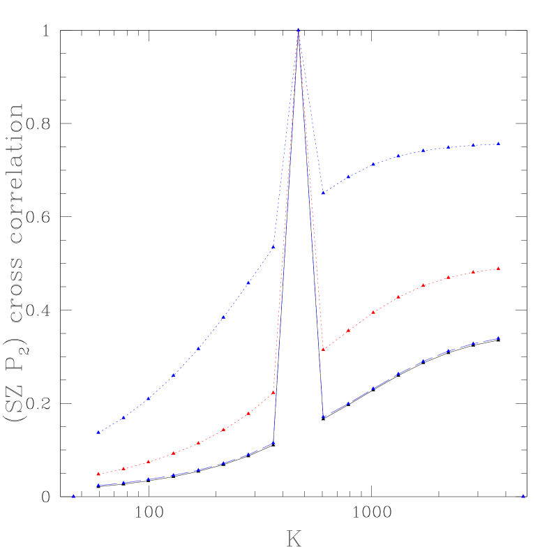
Figure 3: Top: the ratio between the Gaussian and full error for three different choices of $Y_{min}$, $1.7\times 10^{-5},3.4\times 10^{-5},1.0\times 10^{-4}$; top to bottom. Bottom: the cross correlation for the power spectrum, $\langle P_{2}(469)P_{2}(K)\rangle/\sqrt{\langle P_{2}(469)P_{2}(469)\rangle/\langle P_{2}(K)P_{2}(K)\rangle}$ for three different choices of $Y_{min}$, $1.7\times 10^{-5},3.4\times 10^{-5},1.0\times 10^{-4}$, bottom to top. In both figures there is also a line for for the power law example with ${\mathcal{N}}=35000$; it is almost completely degenerate with that for $Y_{min}=1.7\times 10^{-5}$.

The above is for the power spectrum. For the correlation function, the Poisson corrections are small, similar to the power law example. For instance, in estimates pertaining to Planck (e.g. Mei & Bartlett MeiBar03 (2003)) with $Y_{min}=1.0\times 10^{-4}$, the shot noise only approximation to the error is quite good, within the 5% of the full Poisson error for $\theta>30^{\prime}$.

In three dimensions the value of $K$ for clusters is smaller and $\xi(r)$ is larger, so the Gaussian terms become more dominant for the power spectrum and less so for the correlation function. An unbinned power law case is shown here just to illustrate the (large) effects of the full Poisson treatment. Consider a rough power law approximation to the correlation function for galaxy clusters (e.g. Bahcall et al Bahetal (2004), for $M>1\times 10^{14}h^{-1}M_{\odot}$), i.e. take $\xi(r)=100r^{-1.9}$ so that $P(k)=1.9\times 10^{3}k^{-1.1}(h^{-1}Mpc)^{3}$. In figure four, the ratio of the Gaussian to total errors and the cross correlation are shown for the correlation function and the power spectrum, with ${\mathcal{N}}$ = $10^{-3},10^{-4},10^{-5}$. For the correlation function the Gaussian errors differ from the Poisson errors by a factor of $\xi(r)/n_{p}$ and are a less accurate approximation for the correlation function error than in two dimensions.

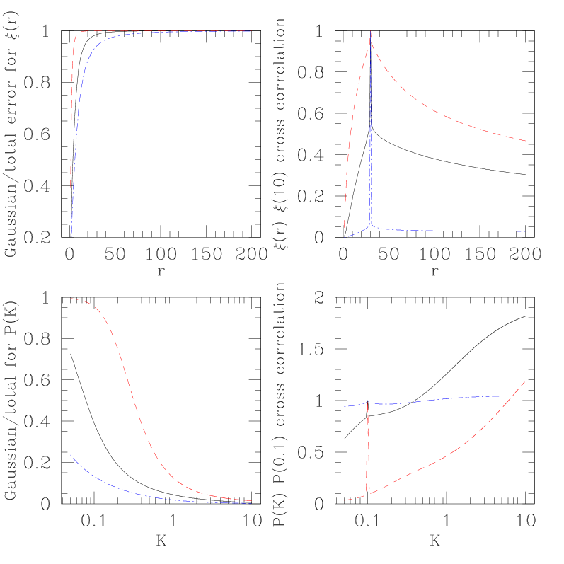
Figure 4: Upper left: the ratio of the Gaussian error to the total error for the three dimensional correlation function. Upper right: the cross correlation $\langle\xi(r)\xi(30)\rangle/\sqrt{\langle\xi(r)\xi(r)\rangle\langle\xi(30)\xi(30)\rangle}$ for the three dimensional power law example. For both, ${\mathcal{N}}=10^{-3},10^{-4},10^{-5}$ top to bottom. Lower left: the ratio of the Gaussian error to the total error and right, the cross correlation $\langle P(k)P(0.1)\rangle/\sqrt{\langle P(k)P(k)\rangle\langle P(0.1)P(0.1)\rangle}$ for the three dimensional power law example. ${\mathcal{N}}=10^{-3},10^{-4},10^{-5}$ top to bottom left, and bottom to top right. No binning is assumed, so the peak in the cross correlation is very sharp.

One expects of order $10^{-4}-10^{-5}$ clusters, with mass above $10^{14}h^{-1}M_{\odot}$ per cubic $h^{-1}Mpc$; if the mass cut is higher the density is lower and the shot noise effects and the correlation function/power spectrum are all larger. The Poisson effects on the error matrix appear to be large unless the shot noise is very small.

For both two and three dimensions, an estimate of when non-Gaussian effects in the (angular) power spectrum itself become important is often given by considering $\Delta_{2}^{2}(k)=\frac{K^{2}P_{2}(K)}{2\pi}$ and $\Delta^{2}(K)=\frac{K^{3}P(K)}{2\pi^{2}}$ in the range $\sim 0.1-1$. For the power law examples considered this is a large range, $650\leq K\leq 5300$ for two dimensions and $0.03\leq K\leq 0.09$ for three dimensions, i.e. there may be other modifications at the scales where the shot noise non-Gaussianity becomes relevant.

5 Conclusions

Poisson shot noise can produce an error matrix for the correlation function and power spectrum significantly different from that calculated in the Gaussian shot noise approximation. The primary contribution to the correlation function error matrix is diagonal and goes as $w(\theta)/n_{p}$ in two dimensions and as $\xi(r)/n_{p}$ in three dimensions. For the power spectrum, there are additions to both diagonal and off-diagonal terms in the error matrix, and thus correlations are introduced in the power spectrum, even for a Gaussian density distribution. For SZ selected galaxy clusters, the errors in the two dimensional correlation function are well approximated by the Gaussian error except for $\theta$ extremely small. For the power spectrum, the cross correlations and additional errors are significant. Binning increases this effect as it reduces the Gaussian contribution relative to the Poisson contributions for the power spectrum. This increase in the error matrix due to the Poisson nature of shot noise should be taken into consideration both for parameter estimation and in survey design (e.g. a shallow survey increases the shot noise and thus these additions to the error and correlations for the power spectrum).

There are two important caveats: The cluster density itself is non-Gaussian at small enough scales and thus at small enough distances these two contributions to the error matrix should be combined. It should be noted that due to non-Gaussianity, the error matrix alone will also be insufficient to calculate the full likelihood. The Poisson shot noise description may also break down in high density regimes (Casas-Miranda et al Casetal02 (2002)). It would be interesting to see the effects of the other non-Gaussian shot noise distributions which appeared in their analysis (sub- and super-Poisson).

The analytic calculations here, just as in the Gaussian shot noise case, are of the most utility in estimating the power of future observations and guiding the corresponding observational strategies. When the eagerly awaited data is in hand, mock catalogues and various statistical strategies such as bootstrap, jack-knife and Monte Carlo (whichever is most appropriate for the question of interest, see e.g. Lupton Lup93 (1993) for an introduction) will likely be needed to include the effects of both the complications discussed in this paper and additional observational aspects such as window functions.

An additional point in this paper is that there is a rewriting of integrals used in the error matrix which eliminates most of the integrals over Bessel and spherical Bessel functions. This reduces much of the dependence of the error matrix on the tails of the power spectrum and correlation functions and also makes the error matrix integrals more tractable.

Acknowledgements: This work was supported in part by NSF-AST-0205935. I thank W. Hu for suggesting the inclusion of Poisson shot noise for galaxy cluster errors. I also thank T.-C. Chang, G. Holder, Y. Lithwick, S. Mei, A. Pope, R. Scranton, R. Sheth, I. Szapudi, R. Wechsler, the anonymous referees, and especially M. White for helpful discussions. I thank R. Sheth for correcting errors in some of the integration measures.

References

• (1) Bahcall, N.A., Hao, L., Bode, P., Dong, F., 2004, Ap J 603, 1
• (2) Bernstein, G.M., 1994, ApJ 424, 569.
• (3) Casas-Miranda, R., Mo, H.J., Sheth, R.K., Borner,G., 2002,MNRAS 333, 730
• (4) Cohn, J., Kadota, K., astro-ph/0409657
• (5) Eisenstein, D., Hu, W., 1997, ApJ 511, 5
• (6) Eisenstein, D. J., Zaldarriaga, M., 2001, ApJ 546, 2
• (7) Evrard, A.E., et al, 2002, ApJ 573, 7
• (8) Geisbusch, J., Kneissl, R., Hobson, M., astro-ph/0406190
• (9) Hamilton, 2000 astro-ph/9905191
• (10) Jackson, A.D. & Maximon, L. C., 1972, Siam J. Math. Anal., 3, 446. http://locus.siam.org/SIMA/volume-03/art_0503043.html
• (11) Landy, S.D., & Szalay, A.S., 1993, ApJ 412, 64L
• (12) Layzer, D., 1956, AJ 61, 383
• (13) Lima, M., Hu, W., 2004, PRD 70, 3504 L
• (14) Lupton, R., 1993, Statistics in Theory and Practice, Princeton University Press, Princeton
• (15) Mei, S., Bartlett, J., 2003, A & A, 410, 767
• (16) Meiksin, A., White, M., 1999, MNRAS 308, 1179
• (17) Peebles,P.J.E., 1980, The Large-Scale Structure of the Universe, Princeton University Press, Princeton
• (18) Sheth, R., Tormen, G., 1999, MNRAS 308, 119
• (19) Van Deun, J., Cools, R., 2006, ACM Transactions on Mathematical Software, Vol. 32, No. 4
• (20) Watson, G.N., 1966, A Treatise on the Theory of Bessel Functions, Cambridge University Press, New York