High-redshift quasar host galaxies with adaptive optics

We present $K$ band adaptive optics observations of three high-redshift ($z\sim 2.2$) high-luminosity quasars, all of which were studied for the first time. We also observed several point spread function (PSF) calibrators, non-simultaneously because of the small field of view. The significant temporal PSF variations on timescales of minutes inhibited a straightforward scaled PSF removal from the quasar images. Characterising the degree of PSF concentration by the radii encircling 20 % and 80 % of the total flux, respectively, we found that even under very different observing conditions the $r_{20}$ vs. $r_{80}$ relation varied coherently between individual short exposure images, delineating a well-defined relation for point sources. Placing the quasar images on this relation, we see indications that all three objects were resolved. We designed a procedure to estimate the significance of this result, and to estimate host galaxy parameters, by reproducing the statistical distribution of the individual short exposure images. We find in all three cases evidence for a luminous host galaxy, with a mean absolute magnitude of $M_{R}=-27.0$ and scale lengths around $\sim 4$–12 kpc. Together with a rough estimate of the central black hole masses obtained from C iv line widths, the location of the objects on the bulge luminosity vs. black hole mass relation is not significantly different from the low-redshift regime, assuming only passive evolution of the host galaxy. Corresponding Eddington luminosities are $L_{\mathrm{nuc}}/L_{\mathrm{Edd}}\sim 0.1$–0.6.

1 Introduction

The study of high-redshift quasar host galaxies has during the past few years become quite an active research field, offering new roads of insight both on the phenomenon of quasar evolution as well as galaxy formation in the early universe. The strong cosmic evolution seen in the quasar population from the peak at $z\sim$ 2–3 is very likely an effect of changing environmental conditions. Together with the evolution in the star formation rate from $z\sim$ 2 to the present, this implies a strong link between the formation and subsequent evolution of galaxies and the processes that trigger and maintain the quasar activity (e.g. Franceschini et al. 1999). This is reflected in the correlation between black hole mass and host spheroid luminosity found for local massive ellipticals (Magorrian et al. 1998; Kormendy & Gebhardt 2001), which has been shown to hold for also quasars (Laor 1998; McLure & Dunlop 2002). Observations of quasar host galaxies over a range of redshifts are necessary to obtain further insights into these links.

It has been repeatedly predicted that the observational technique of adaptive optics (AO) could be pivotal in the advancement of quasar host galaxy research, because of its greatly enhanced angular resolution. AO observations are already successfully employed for the imaging of, e.g., protoplanetary disks and binary star systems, but it is probably fair to say that there are still only very few applications to quasar hosts. One reason for this could well be due to an inherent property of AO images of point sources, namely the superposition of a diffraction-limited core with an extended halo. Operating at low Strehl ratio (often unavoidable at high Galactic latitudes where bright guide stars for wavefront sensing are scarce) greatly enhances this problem. Furthermore, accurate knowledge of the point spread function (PSF) is a prerequisite. However, the high spatial sampling of AO detectors is always paid for with a small field of view, and non-simultaneous PSF observations often cannot be avoided. As a consequence, the fundamental task of correctly differentiating between a compact nucleus and an extended host galaxy remains a challenge.

Most of the existing AO data on quasar hosts was obtained in the near-infrared $K$ band, where the effects of atmospheric turbulence are less pronounced than at shorter wavelengths. In the case of low to intermediate redshift quasars, the host galaxies are easily resolved, and the PSF details were not crucial to the detection of the objects (Stockton et al. 1998; Márquez et al. 2001); rather, the main emphasis was on the detection of structural details. This is different at high redshifts ($z\ga 1$) where the detection of the host galaxy as such becomes again a challenge, even with AO (Aretxaga et al. 1998; Hutchings et al. 2001; Lacy et al. 2002; Croom et al. 2004; Falomo et al. 2005). Other ground- and space-based campaigns with high resolution were also successful in resolving host galaxies to $z\sim 2.5$ (Kukula et al. 2001; Jahnke et al. 2004b; Falomo et al. 2004), or even $z\ga 4$ (Hutchings 2003).

The focus of the present paper is on high-luminosity quasars around and slightly above $z\sim 2$, with the aim of constraining the host vs. nuclear luminosity (and black hole mass) relations at these redshifts. Although we used an AO instrument/telescope combination that has been decommissioned since, published AO observations of high-$z$ quasars are still so scarce that even our small sample makes a non-negligible contribution to the field. Moreover, we have spent considerable effort at analysing the effects of temporal PSF variability, and designed a method to infer on quasar host properties with non-simultaneously obtained PSF observations. Besides our astrophysical results, we hope that some of the methodical insights and strategic aspects mentioned in this paper may be of interest to the community.

We first present our set of new targets in Sect. 2, together with a summary of the AO observations and data reduction. Section 3 is dedicated to the task of image quality assessment, emphasising the aspects of temporal PSF variability. In Sect. 4 we describe our analysis strategy, based on extensive simulations designed to reproduce the observed image characteristics. The results of applying this method to our data are presented in Sect. 5, which we discuss in astrophysical context in Sect. 6. Throughout this paper we adopt $H_{0}=70$ km s^-1 Mpc^-1, $\Omega_{m}=0.3$ and $\Omega_{\Lambda}=0.7$. All magnitudes are zeropointed to the Vega system.

2 Targets

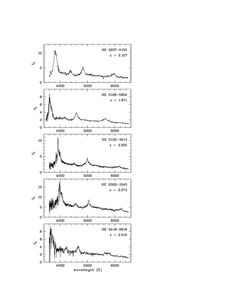
Figure 1: Slit spectra of the five newly discovered quasars, taken with ESO telescopes. See text and Table 1 for details. $f_{\lambda}$ is in units of $10^{-16}$ erg cm^-2 s^-1.

Figure 2: $2^{\prime}\times 2^{\prime}$ DSS images around the five featured quasars (the central object in each panel), together with their corresponding AO guide stars. North is up, East is to the left.

Table 1: Basic properties of the input target sample quasars, PSF stars, and the corresponding adaptive optics guide stars. Column 5 gives $B_{J}$ band magnitude for the quasars and $V$ band magnitude for the PSF stars. The last three PSF stars were observed unrelated to any of the quasars.

Object name	R.A. (J2000.0) Dec		$z$	$B_{J}$/$V_{\star}$	Guide star	distance	$V_{\star}$
HE 0037$-$5155	$00^{\mathrm{h}}\>40^{\mathrm{m}}\>17\aas@@fstack{s}1$	$-51\degr\>38^{\prime}\>49^{\prime\prime}$	2.127	17.7	GSC0803000529	16$\aas@@fstack{\prime\prime}$8	12.9
GSC0802400921	$00^{\mathrm{h}}\>37^{\mathrm{m}}\>34\aas@@fstack{s}7$	$-47\degr\>19^{\prime}\>44^{\prime\prime}$		14.8	GSC0802400297	15$\aas@@fstack{\prime\prime}$2	13.0
GSC0803000534	$00^{\mathrm{h}}\>41^{\mathrm{m}}\>21\aas@@fstack{s}7$	$-52\degr\>28^{\prime}\>00^{\prime\prime}$		15.6	GSC0803000242	13$\aas@@fstack{\prime\prime}$2	13.8
HE 0108$-$5952	$01^{\mathrm{h}}\>10^{\mathrm{m}}\>52\aas@@fstack{s}0$	$-59\degr\>36^{\prime}\>21^{\prime\prime}$	1.971	18.9	GSC0847901239	25$\aas@@fstack{\prime\prime}$2	12.0
HE 0132$-$3013	$01^{\mathrm{h}}\>34^{\mathrm{m}}\>33\aas@@fstack{s}8$	$-29\degr\>58^{\prime}\>15^{\prime\prime}$	2.229	18.0	GSC0642801994	28$\aas@@fstack{\prime\prime}$8	11.0
GSC0642602115	$01^{\mathrm{h}}\>26^{\mathrm{m}}\>21\aas@@fstack{s}8$	$-25\degr\>49^{\prime}\>46^{\prime\prime}$		14.6	GSC0642601594	26$\aas@@fstack{\prime\prime}$1	11.5
GSC0700200978	$01^{\mathrm{h}}\>19^{\mathrm{m}}\>57\aas@@fstack{s}9$	$-30\degr\>44^{\prime}\>50^{\prime\prime}$		15.5	GSC0700200865	27$\aas@@fstack{\prime\prime}$2	11.7
HE 0320$-$1045	$03^{\mathrm{h}}\>22^{\mathrm{m}}\>24\aas@@fstack{s}5$	$-10\degr\>35^{\prime}\>12^{\prime\prime}$	2.282	17.0	GSC0529800301	18$\aas@@fstack{\prime\prime}$0	13.0
GSC0530900226	$03^{\mathrm{h}}\>39^{\mathrm{m}}\>24\aas@@fstack{s}1$	$-12\degr\>39^{\prime}\>49^{\prime\prime}$		14.9	GSC0530900199	15$\aas@@fstack{\prime\prime}$6	13.5
GSC0529400760	$03^{\mathrm{h}}\>05^{\mathrm{m}}\>37\aas@@fstack{s}7$	$-08\degr\>02^{\prime}\>02^{\prime\prime}$		14.8	GSC0529400764	19$\aas@@fstack{\prime\prime}$9	13.2
HE 0418$-$0619	$04^{\mathrm{h}}\>21^{\mathrm{m}}\>24\aas@@fstack{s}2$	$-06\degr\>12^{\prime}\>04^{\prime\prime}$	2.010	19.0	GSC0473301854	15$\aas@@fstack{\prime\prime}$6	11.9
GSC0472901414	$04^{\mathrm{h}}\>11^{\mathrm{m}}\>08\aas@@fstack{s}3$	$-03\degr\>46^{\prime}\>53^{\prime\prime}$		13.8	GSC0472901410	16$\aas@@fstack{\prime\prime}$7	13.1
GSC0548301352	$09^{\mathrm{h}}\>54^{\mathrm{m}}\>37\aas@@fstack{s}1$	$-11\degr\>18^{\prime}\>32^{\prime\prime}$		14.3	GSC0548301353	26$\aas@@fstack{\prime\prime}$2	11.6
GSC0490901021	$10^{\mathrm{h}}\>00^{\mathrm{m}}\>44\aas@@fstack{s}5$	$-07\degr\>01^{\prime}\>05^{\prime\prime}$		14.6	GSC0490901030	26$\aas@@fstack{\prime\prime}$6	11.8
GSC0490900476	$10^{\mathrm{h}}\>04^{\mathrm{m}}\>58\aas@@fstack{s}0$	$-05\degr\>17^{\prime}\>44^{\prime\prime}$		14.9	GSC0490900457	27$\aas@@fstack{\prime\prime}$9	11.7

2.1 Target selection

The number of high-redshift quasars bright enough to allow on-axis adaptive wavefront correction is extremely small. It is basically zero for the more venerable AO systems such as ADONIS on the ESO 3.6 m telescope used by us (see below). In line with other researchers, we have therefore searched for targets with a nearby bright star that can be used for wavefront sensing. For ADONIS, the uttermost limits for AO correction in the $K$ band were: a red ($R$ or $I$) stellar magnitude $\la 13$, and a distance between quasar and star of $\la 30^{\prime\prime}$; to be practical, these two criteria should not be carried to their extremes together. Even then, the low surface densities of pairs of quasars and stars fulfilling both conditions make the number of such targets necessarily small in any survey. Other groups before us already used the available quasar catalogues to identify possible targets, and at the time of planning this project in 1999, these catalogues seemed to be more or less exhausted, at least to the limits of systems such as ADONIS.

We therefore performed a new search using the largely unexplored database of optically bright quasars from the Hamburg/ESO survey (HES, Wisotzki et al. 2000), containing several thousand bright quasars and quasar candidates at all redshifts up to $z\simeq 3.2$. The survey magnitude limit of $B_{J}\la 18$ (on average) makes it a rich source of high-luminosity quasars. We went through the full database, selecting all quasars with redshifts $z\ga 1.8$, and included also quasar candidates where a tentative redshift had been assigned based on their digitised objective prism spectra (for details, see Wisotzki et al. 1996, 2000). We then paired the list with the HST Guide Star Catalogue (GSC) and searched for pairs matching the above given criteria for possible ADONIS guide stars with $B_{J}<14$. Altogether, we arrived at 12 candidate targets selected by these criteria. Of these, seven objects strained both the magnitude and the distance limits to an unacceptable degree and were eliminated from the list. We were then left with five remaining targets that we eventually took to the telescope.

All of these five quasars appear here for the first time in the literature. The data for them are given here for the benefits of the community, as we believe that they might be interesting to other groups working in the field of quasar host galaxies and adaptive optics in the future. Table 1 contains their basic properties, including those of the adopted AO guide star. The quasars are drawn from an optical survey, and no radio flux measurements of the sources exist; they are most likely radio-quiet. We show slit spectra of the quasars in Fig. 1, taken with either the ESO 1.52 m or the ESO/Danish 1.54 m telescope between 1996 and 2000. Further below in this paper we use these spectra to obtain a rough estimate of the black hole masses in these objects. Finally, Fig. 2 shows postage stamp images of the quasars together with their nearby AO guide stars.

2.2 PSF calibrators

In order to obtain photometry and morphological parameters of a quasar host galaxy, the contribution of the point-like active nucleus has to be removed, for which an accurate knowledge of the PSF is essential. In our case with a field of view of only $12\aas@@fstack{\prime\prime}8\times 12\aas@@fstack{\prime\prime}8$, the quasars were in all cases completely isolated, and we were forced to obtain constraints of the PSF from external stellar calibrators, to be observed non-simultaneously with the quasars. (Even if there had been useful stars inside the field of view, the inevitable spatial PSF variations over the isoplanatic patch would have made their use highly questionable.)

We decided to accompany each quasar with two different PSF calibrators, to enable cross-validation. Each of these PSF calibrator stars were selected to have a wavefront sensing guide star of magnitude and distance as closely matching to that of the quasar guide star as possible (see Table 1).The PSF stars themselves were chosen to be substantially brighter than the quasars, typically around $B_{J}\simeq$ 14–15, allowing for a high S/N PSF definition with a small number of exposures. Following these criteria, we selected several stellar pairs from a $\sim 5\degr$ surrounding of each quasar.

2.3 Observations

Observations were performed in the $K_{s}$ band on the nights of 1999 November 27–29, using the ADONIS system on the ESO La Silla 3.6m telescope. The SHARPII+ camera was equipped with a 256$\times$256 Nicmos III array with a pixel size of 40 $\mu$m. The pixel scale was set to 0$\aas@@fstack{\prime\prime}$05/pixel, resulting in a field of view of $12\aas@@fstack{\prime\prime}8\times 12\aas@@fstack{\prime\prime}8$. Because of variable weather conditions we concentrated on only three of our targets: HE 0037$-$5155, HE 0132$-$3013, and HE 0320$-$1045.

For every target the quasar itself was first observed in a cycle of $10\times 60$ or $15\times 60$ seconds, followed by the corresponding two PSF stars in a cycle of $3\times 60$ seconds per object. Each individual frame of 60 s exposure (which in turn consisted of ten 6 s detector integration cycles) was saved and used in the later analysis. Photometric standard stars were obtained at the beginning and end of each night, and skyflats were acquired in evening twilight. The seeing as computed from the wavefront sensing data by the ADONIS instrument software was stable at $\simeq 0\aas@@fstack{\prime\prime}6$ during the first night, but varied between 0$\aas@@fstack{\prime\prime}$7–1$\aas@@fstack{\prime\prime}$1 and 0$\aas@@fstack{\prime\prime}$8–1$\aas@@fstack{\prime\prime}$2, respectively, during the useful portions of the following two nights.

To monitor the variable sky background, we used the standard option of switching back and forth between two locations of the quasar on the chip $\sim$8″ apart, using the internal chopping mirror. Total integration times amounted to 160 min for HE 0037$-$5155, 170 min for HE 0132$-$3013, and 230 min for HE 0320$-$1045, while each of the PSF stars was typically integrated for 36 min total.

2.4 Reduction

After bias subtraction and flatfielding, each stack of consecutive 1 min integrations of a single target was recorded in two image cubes, separating odd- and even-numbered frames. Each frame set was averaged separately. The odd-numbered average was then adopted as sky background estimate for the stack of even-numbered images and subtracted, and vice versa. Since each average frame contained also the quasar image in the opposite quadrant, the subtraction creates a negative imprint of the quasar in all individual frames (Fig. 3). This was not a problem since we used only the quadrant with the quasar in it for further analysis.

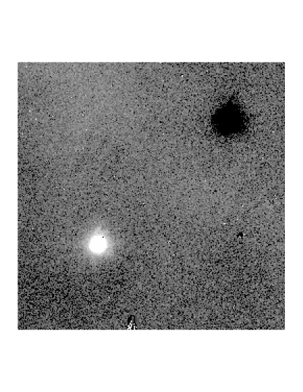
Figure 3: Example of a background corrected image from an image cube of HE 0037$-$5155. The quasar is located in the lower left corner, while the opposite corner contains a negative residual from the alternate chopping position.

After subtraction of the background frame, some lower level residual structure remained that was created by different thermal emission patterns from the two positions of the chopping mirror (see Eisenhauer 1997). Since only a small detector area covered by the quasar light distribution with a diameter of $\sim 2^{\prime\prime}$ was needed for analysis, we assumed the background to be locally constant. The level of this local background was then fine-tuned by demanding a constant radial curve of growth between 1″and $1\aas@@fstack{\prime\prime}5$ radius. This is a conservative procedure; some small fraction of quasar flux was clearly still present within this range, and we are thus slightly biased against the detection of extended emission. Using simulations, we estimated this effect to be less than 0.1 mag for all realistic host galaxy models. Increasing this radius would have decreased the systematic error, but at the same time it would have enhanced the vulnerability to small-scale residual sky variations on an amplitude comparable to the local object flux.

For all reduced frames we created bad pixel maps from skyflats using the ‘flat’ task from the ECLIPSE data reduction package (Devillard 2001). It was found that bad pixel areas changed in size within image cubes, so a global bad pixel map was therefore complemented with individual maps for each frame where also cosmics were marked. The remanence effect common for Nicmos III arrays (which alters the sensitivity of pixels over- or underexposed in the previous frame) was found to be negligible for both quasar and PSF star images. Photometric calibration was performed by aperture photometry on the standard stars. The uncertainty of the calibration is 0.05 magnitudes. Finally, the quadrant containing the quasar was extracted from each reduced image cube. During data reduction we found that some single images or whole image cubes (of both quasars and stars) were badly affected by problems with the AO optimisation loop or with the guiding. These data were excluded from subsequent analysis.

Figure 4: Progression of core width with time. In the top panel we plot average values and $1\sigma$ error bars for each image cube for both PSF calibrator stars (filled diamonds) and quasar observations (circles). We expand the beginning of the second night in the lower panel, plotting values for every image of the first five cubes. The width variation between two consecutive images can be as large as 30 %.

3 The point spread function

3.1 Image quality assessment and PSF variability

As laid out in Sect. 2.2 above, we had to rely on PSF calibrator stars observed non-simultaneously, but with configurations very similar to the quasar observations. A major concern with this approach lies in the fact that under permanently changing ambient conditions, the PSF itself is expected to vary with time. In order to monitor and assess the temporal variability of the PSF, the observations of PSF calibrator stars and quasars were nested.

Because of the nearly diffraction-limited core of AO images, the full-width at half maximum (FWHM) is not a very sensitive image quality indicator. A better quantity is the Strehl ratio $S$, which however is difficult to determine for quasar images because of the possible contribution of the host galaxy. We adopted as ‘core width’ indicator the radius $r_{20}$ encircling 20 % of the total flux of the object. For point sources, we found that $r_{20}$ is closely related to the Strehl ratio, following the approximate relation $S\approx 0.52-0.32\>(r_{20}/1^{\prime\prime})+0.056\>(r_{20}/1^{\prime\prime})^{2}$. The variation of $r_{20}$ is plotted in Fig. 4. Typical core widths are near 0$\aas@@fstack{\prime\prime}$05 or slightly above, corresponding to Strehl ratios of around 0.2 (ranging from below 0.1 to above 0.3).

Unfortunately, we found the PSF to be significantly variable even within single image cubes, over lapses of 30 min or less. The reason for the variability of the PSF is the rapid change of the atmospheric turbulence characteristics, inducing different responses from the AO system. This in turn leads to variation in the centroid, higher FWHM, lower Strehl ratios and higher speckle noise. An increase in integration time, or coaddition of several images, would in general reduce this variation but will at the same time decrease resolution and hence the benefits of AO observation (cf.  Le Mignant et al. 1998). In the $K_{s}$ band, exposure times are in any case limited by the strong sky background emission in order to avoid non-linearity or saturation effects. Since the variations also apply to PSF star images displaying similar Strehl values, thus suggesting very similar correction quality of the AO system, we have to conclude that the PSF in any individual quasar image is essentially unknown, and can only be estimated by statistical means.

This posed a serious problem, as standard methods of quasar host analysis can only be applied to AO data when the hosts are very extended and the knowledge of the exact shape of the PSF is less important. While this is usually the case for low-$z$ quasar when structures outside of the centre are to be resolved, the situation is different for high-$z$ quasars. It is clear that another approach was needed to evaluate whether an observed quasar is extended or not, and to determine the characteristics of the possible host galaxies.

In order to describe the image PSF we first investigated the most prominent variation: the variation of image concentration.

3.2 Image concentration diagnostics

While the PSF variation in general is probably not predictable, we considered the question whether at least some simplified shape descriptor might show some regularity. Figure 5 displays the relation between the width of the core and the width of the wings, as measured by the radii including 20 % and 80 % ($r_{80}$) of the flux, for all individual 1 min PSF star observations. The data clearly follow a – slightly non-linear – trend, which we approximated with a parametrised polynomial fit in Figure 5. This fit will be called the ‘PSF track’ henceforth. Notice that we use both values $r_{20}$ and $r_{80}$ rather than just their ratio as a ‘concentration index’ to allow for more freedom in describing the observed shape variations.

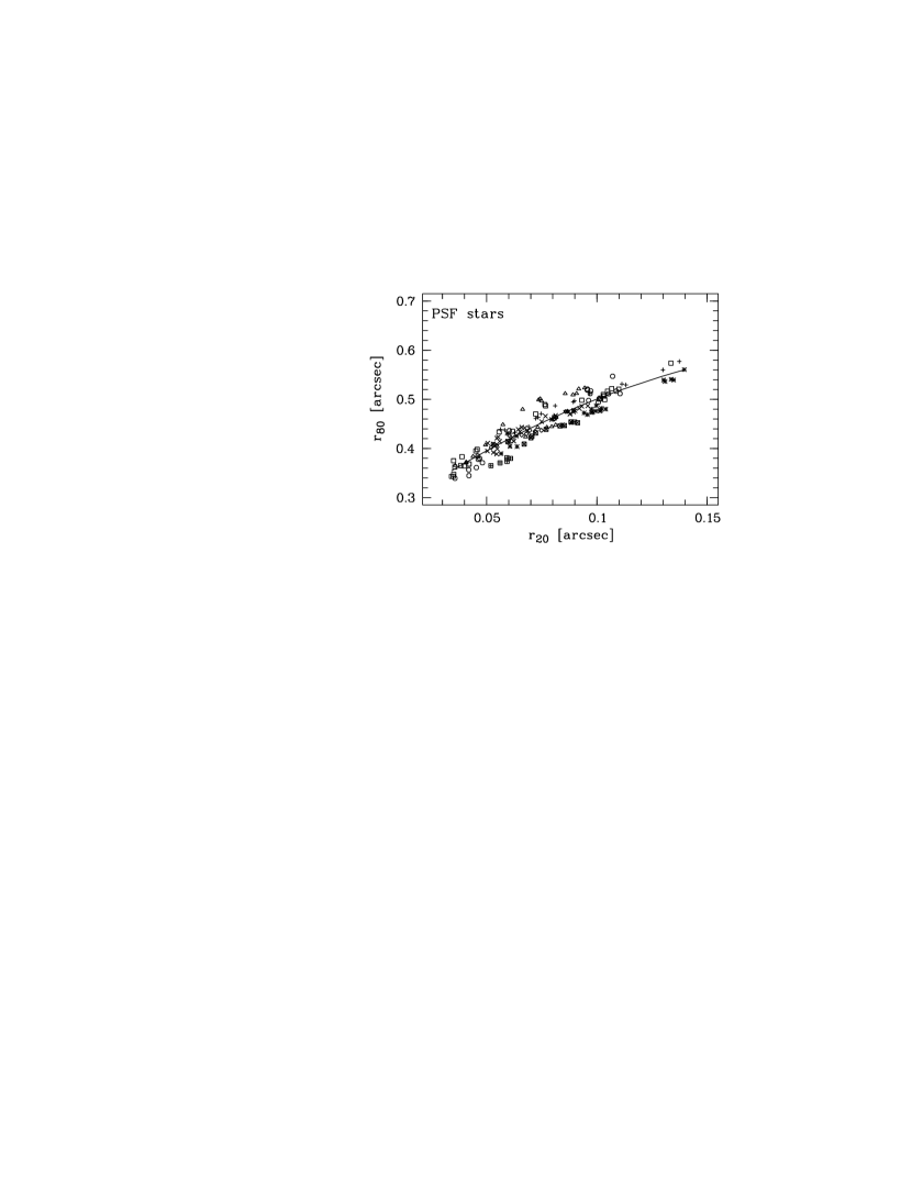
Figure 5: The $r_{20}$–$r_{80}$ diagram for the PSF stars. Each point corresponds to a single 1 min image from an image cube. Different individual PSF stars are coded with different symbols. The solid line is the best fit to the PSF star points (‘PSF track’). The variation due to different observing conditions is generally larger than the difference between individual PSF stars.

Remarkably, Fig. 5 contains data taken under very different ambient conditions, with guide stars of different brightnesses and with different AO optimisation settings; nevertheless, the relation is rather tight. The main reasons for the scatter of individual frames around this are photon shot noise and variable two-dimensional asymmetries in the PSF shape, in proportions depending on the brightness of the object. The PSF star–guidestar configuration has much less influence on the position of the observations in the $r_{20}$–$r_{80}$ diagram than the observing condition. This can well be seen in PSF stars which were observed in several nights, e.g. GSC0642602115 (coded by triangles) which is placed both above and below the PSF track.

Given that the PSF can be characterised by such a simple relation, we now demonstrate that the same diagnostic can be used to search for faint extended emission underlying a bright quasar image. Figure 6 shows the curves of growth of both a PSF star and of a quasar. While both are dominated in their cores by the PSF, thus having virtually identical $r_{20}$ values, the host galaxy contributes fractionally more flux to the wing, thus flattening the curve of growth and increasing $r_{80}$.

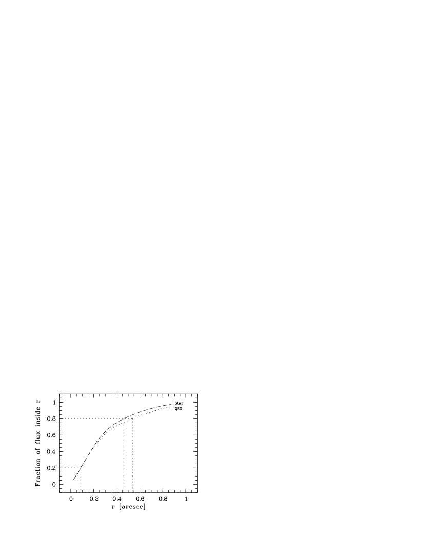
Figure 6: Growth curves for a star (dashed line) and a quasar (dotted line), taken from the first cubes of the second night (lower panel in Fig. 4). The determination of $r_{20}$ and $r_{80}$ radii allows a distinction between the two types.

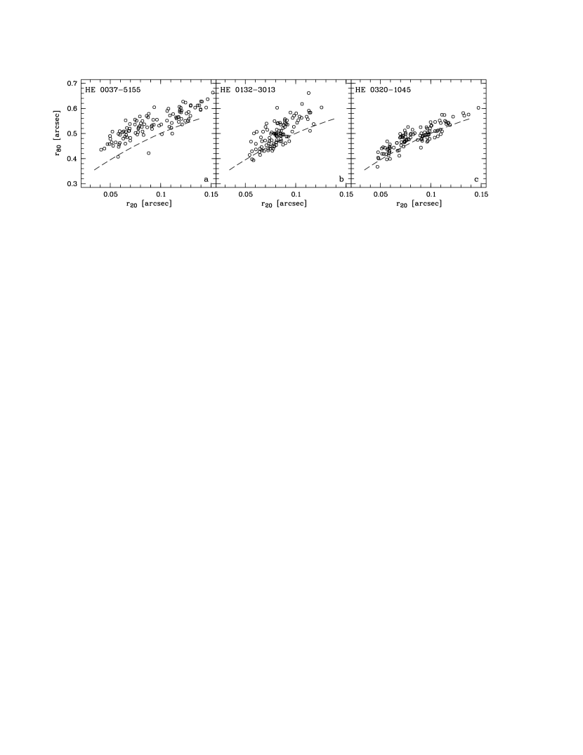
Figure 7: The $r_{20}$–$r_{80}$ diagrams for the quasars. Each point corresponds to a single image from an image cube. The dashed line is the fitted ‘PSF track’ from Fig. 5.

In Fig. 7 we plotted $r_{80}$ vs. $r_{20}$ for all individual 1 min quasar images of the three nights. We show the distribution of points for the three quasars separately (Figs. 7 a–c), where it can be seen that for none of them the points scatter around the fitted PSF track. In the cases of HE 0037$-$5155 and HE 0132$-$3013 the offset between points and line appears significant even at first glance, whereas for HE 0320$-$1045 the effect is less pronounced and debatable. Notice that the quasars show a much higher scatter than the PSF stars in Fig. 5; this is expected, since the stars are typically ten times brighter than the quasars. This implies that the scatter in the quasar images is dominated by shot noise.

The shift of the quasars away from the PSF track in these diagrams is immediately suggestive of influence from a host galaxy, but in order to quantitatively confirm a detection, we need a better understanding of the principles which create the distribution of points in the diagram. To this end we will in the following attempt to reconstruct the distribution of quasars in these diagrams using our knowledge about the distribution of PSF star points under the hypothesis that the presence of a host galaxy is responsible for the observed shift. This is done in three steps, by investigating each of the following questions in turn:

• Can the offsets of the quasar images be explained by adding host galaxy flux to a point source?

• Is one galaxy model able to explain the average $r_{20}$–$r_{80}$ relation for a given quasar?

• Can the entire distribution of quasar data points be represented with a set of simulations created to match the actual conditions of observation?

4 Simulations

4.1 Individual images

To simulate a single quasar observation, we created artificial quasar nuclei with surrounding host galaxies as would be observed under different external conditions, and studied their behaviour in the $r_{20}$–$r_{80}$ diagram. The artificial objects were composed of the observed image of a PSF star to represent the nucleus, plus a model galaxy. The numerical model we use is the well-known spheroidal law by de Vaucouleurs (1948):

$$F_{\mathrm{sph}}(r)=F_{\mathrm{sph},0}\,\exp\left[-7.67\,\left(\frac{r}{r_{50}}\right)^{1/4}\right],$$ (1)

where $r_{50}$ is the radius which encircles half the total flux.

We chose the spheroidal model since it is not unreasonable to expect highly luminous quasars to be hosted by ellipticals (McLeod & Rieke 1995; Dunlop et al. 2003). Even if the host galaxies at high redshifts are more disturbed, the above law can still be considered appropriate as a description of the main part of the flux (e.g. Hutchings et al. 2002), since low surface brightness disk components or tidal features are likely to be missed anyway. Even in the case of a true disk-type host we probably could not distinguish it from an elliptical of similar size and brightness.

We varied the half-light radius $r_{50}$, but restricted the tests to circularly symmetric galaxies for simplicity. The models were numerically convolved with an empirical PSF given by an arbitrary PSF star image, to create a light distribution consistent with the external conditions. Star and convolved object were then scaled and added to mimic different ratios of nuclear to galaxy flux.

The outcome can be seen in Fig. 8. Each tickmark along the solid lines marks the position of an individual simulated image in the $(r_{20},r_{80})$ parameter space. The images along a given solid line were constructed having the same flux ratio between nucleus and host galaxy. They differ only in the PSF star image used in their construction, hence only in external observing conditions. After creation, the simulated data was processed in a manner identical to the real data to extract the $r_{20}$ and $r_{80}$ parameters (the data for HE 0037$-$5155 is overplotted in Fig. 8 for comparison). The different solid lines correspond to sets of simulations with different ratios of nuclear to host flux (n/h). This simulation shows that the artificial quasars, in principle, cover the same region in the $r_{20}$–$r_{80}$ diagram as the real objects.

4.2 Image ensembles

Since neither the nucleus nor the host galaxy vary intrinsically during the observation time span, there must be one galaxy model, viewed under different observing conditions, that is sufficient to represent the distribution of a quasar observation.

In Fig. 8 we show the result for model galaxy half-light radii of 2.4, 7 and 20 kpc, using fifteen different PSF star images to represent the range of observing conditions, and six different flux ratios n/h. The PSF star images were selected to be close to the PSF track (we shall relax that condition in the next subsection) and to be spaced roughly equidistantly along the PSF track. The tickmarked lines in the plot show the set of $r_{20}$–$r_{80}$ values extracted for each artificial object class. The further away a line lies from the PSF track, the lower is the n/h ratio, and thus the higher is the host galaxy flux.

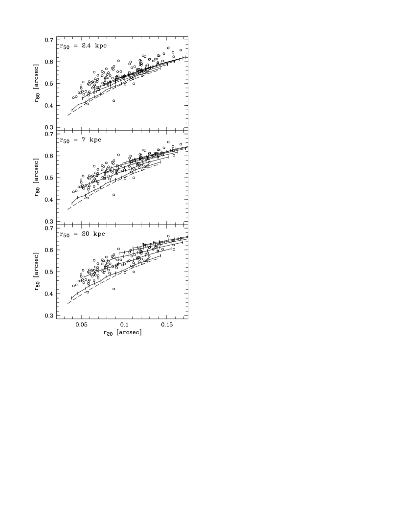
Figure 8: Loci for artificial objects with three different model galaxy scale lengths, plotted on top of the data for HE 0037–5155. The scale lengths were computed at the redshift of the quasar. The dashed line is the PSF track, and the solid lines represent different ratios of nucleus to host flux with the tickmarks showing the location of each object. The n/h ratios are 7.7, 1.5, 0.66, 0.38, 0.23 and 0.16, counting from the bottom to the top.

With increasing host galaxy flux, the lines of constant n/h ratio flatten, and they move upwards and to the right in the $r_{20}$–$r_{80}$ diagram. This flattening can be understood when considering the locus of the extreme case of a pure galaxy without any nucleus. In the limiting case of very bad seeing (high $r_{20}$ values), any galaxy will become unresolved, and galaxy and star become indistinguishable. Thus the ‘pure galaxy line’ and the PSF track join. When external conditions improve, the $r_{20}$ values become smaller and the galaxy starts to be resolved. The difference in $r_{80}$ between point source and galaxy increases, resulting in a flatter slope for the pure galaxy line than for the PSF track. Since the different n/h flux ratios move in between the extremes of ‘galaxy only’ and ‘nucleus only’, they fill the range between the two lines, flattening with increasing relative flux contribution from the host.

At this point we can make our first quantitative statement, based on the observed data: Small host galaxies with a half-light radius of only 2.4 kpc are not able to explain the extended flux we measure in HE 0037–5155. However, answering the initially posed question whether one host galaxy model is enough to explain the observed distribution is harder.

4.3 Including noise

At this stage of the analysis we need to investigate how photon shot noise translates into uncertainties in $(r_{20},r_{80})$ parameter space. It can be expected that noise will influence both parameters, but a priori the size and orientation of the joint error ellipses is unknown. Without this knowledge it is only possible to give a rough estimate of the n/h flux ratio and possible host galaxy radius. One might assume that one of the lines in Fig. 8 could provide a good fit, but for a quantitative answer we need to include random noise effects into the simulations.

In order to do this, artificial objects were created in the same way as before, but these were matched to both the flux of the observed quasar images as well as to their noise properties. To investigate the scatter expected for any constant n/h flux ratio, we selected five intervals in $r_{20}$ typically containing 7–8 stellar images each. Each of these sets shows some scatter around the PSF track which represents the uncertainty about the details of the PSF in the presence of shape variations. Shot noise will be less important for the high S/N PSF star images. After randomly assigning one of the matching PSF star images and adding Gaussian noise to each artificial object in a given $r_{20}$ slice, the artificial quasars contain both the background noise and the PSF shape variation.

For each object in a slice we computed 100 different noise realizations, leading to 100 individual pairs of $r_{20}$ and $r_{80}$. Plotted into the $r_{20}$–$r_{80}$ diagram, the scatter can be roughly quantified as a tilted error ellipse as shown in Fig. 9. We computed these error ellipses for both the so far assumed best-fitting galaxy for each object, and for the null hypothesis of no detectable host galaxy flux contribution. We did this for all three quasars individually since their S/N ratios differ significantly, and since we did not wish to assume a priori that the shape of the error ellipses were independent of S/N or flux ratio (which it however turned out to be).

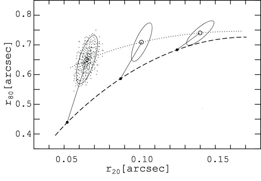
Figure 9: Determination of error ellipses. Adding an artificial galaxy component to a stellar image on the PSF track (dashed curve) shifts the location of the object upwards and to the right, as indicated by the open circles. These are connected by a line of constant n/h flux ratio for a given quasar (dotted curve). When noise is included, the distribution is widened to a cloud of points. The ellipses show the size and orientation of the derived 2$\sigma$ contours.

The scatter in $r_{80}$ is dominated by the shot noise in the quasar images, while the spread in $r_{20}$ is mainly attributable to the width of the stellar $r_{20}$-slices, thus in the uncertainly of the adopted PSF. Scatter along the minor axis can therefore be reduced if more stellar images are available in the simulations, whereas scatter along the major axis can only be reduced by acquiring quasar observations with higher S/N.

An important diagnostic is the orientation of the error ellipses relative to the ($r_{20}$,$r_{80}$) axes. Since noise will shift all points preferentially along the major axis of the corresponding ellipse, these can now be used to backtrace each observed data point to the most probable intrinsic location on a given constant n/h line from where it was scattered. Combined with the knowledge of which – nearly shot-noise free – PSF star image was used to construct the error ellipse at this location, we can assign a unique $r_{20}$ value (that of this PSF star) to each quasar data point. This is taken as a representation of the most probable observing conditions under which the data was taken. We stress that the reason for this exercise is not to try to remove noise from an actual observation, which is obviously impossible, but to reveal the underlying distribution in $r_{20}$–$r_{80}$ space of the point sources which were folded into the quasar images.

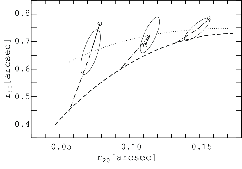
Figure 10: Identifying the most probable PSFs for three given (observed) quasar images, marked by the open circles. Lines are denoted as in Fig. 9. Assuming a specific n/h flux ratio, there is one error ellipse for each quasar with the major axis pointing towards it. From the centre of that ellipse we can point at the corresponding point source location on the PSF track, using the simulations as in Fig. 9.

In Fig. 10 this task is sketched schematically. Recall that we assume to have a best-guess constant n/h flux ratio which allows us to draw the corresponding curve. The first objective is to estimate the position on the constant n/h track from which the data point was most probably scattered. Each data point could, in principle, be derived from any point on the track, but there is only one error ellipse with its major axis directed towards the data point in question. The centre of that ellipse represents the most probable intrinsic $r_{20}$ value. We also know from the simulations which corresponding point source underlies this particular error ellipse, and we know the position of this point source on the PSF track. Hence, we can derive a ‘reduced $r_{20}$ value’ $r_{20,\mathrm{red}}$ of the quasar image.

By doing so for all quasar observations, we can construct the distribution of $r_{20,\mathrm{red}}$ values which essentially allows us to estimate the distribution of observing conditions for a given set of quasar images (cf. Fig. 11). By selecting a subsample of stellar images that has the same distribution in $r_{20}$ as the $r_{20,\mathrm{red}}$ values of a given quasar, we can now create fine-tuned simulations having the same flux, the same noise amplitude, and the same statistical PSF variation properties as the real quasar. We can then proceed to quantitatively test the initial hypothesis of assuming a certain n/h flux ratio by comparing the distribution of observed and simulated $r_{20}$ and $r_{80}$ values, e.g. by means of the standard Kolmogorov-Smirnov test. We perform such tests for our objects in Sect. 5 below.

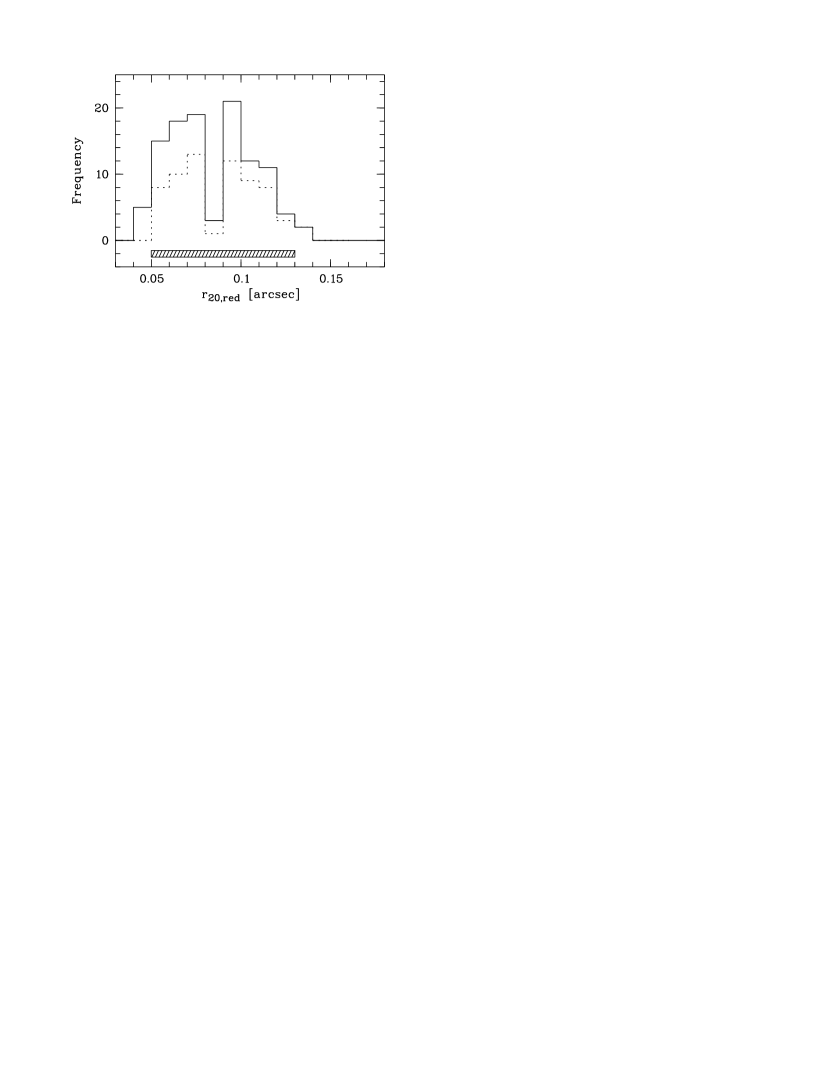
Figure 11: Distribution of $r_{20,\mathrm{red}}$ values for HE 0320$-$1045 (solid line), and distribution of $r_{20}$ values for the selected matched sample of stellar images (dashed line). The distributions agree very well in the range containing a sufficient number of stellar images (indicated by the hashed bar).

5 Analysis of the individual quasars

The procedure outlined above provides a recipe how to test the hypothesis that a given host galaxy model is compatible with the observations. It does not provide a fitting scheme, at least not in the strict sense. However, we can perform this test for several model parameters and thus constrain the range of compatible models. We also include the null hypothesis that no host galaxy is detectable, and that the observed scatter is compatible with pure noise.

Before we proceed to these tests, we briefly touch on some preliminary considerations. Firstly, we note that the recipe to reconstruct the $r_{20,\mathrm{red}}$ values of the quasars relies on all quasar images to have a matching PSF star image to be paired with. A small number of our quasar images were obtained under exceptionally good conditions (small $r_{20}$) for which no matching PSF can be found. A similar though less clear-cut situation occurs at very large $r_{20}$. For the statistical tests we therefore deselected the extreme tails of the $r_{20}$ distribution, using only a limited range of values as indicated by the hashed bar in Fig. 11. This meant that we had to effectively throw away some of our best quasar images, but at the gain of now having a clean matched dataset.

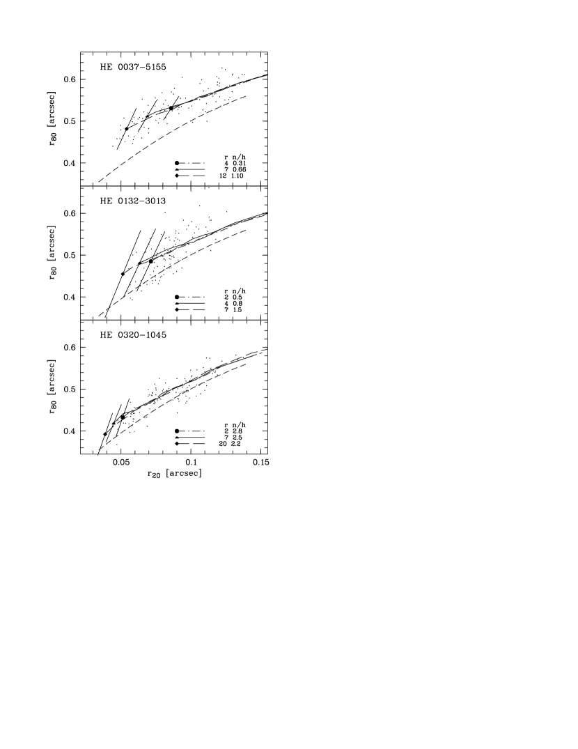
Figure 12: Comparison of different models for the three quasars. The solid curve shows the best-fit model, the dashed and dot-dashed curves show two models with bracketing values of the half-light radius. The beginning of each curve is marked by a filled symbol and a 2$\sigma$ error bar pointing along the major axis of the error ellipse.

From Fig. 8 it is evident that our observations do not provide strong constraints on host galaxy scale lengths. There is a significant degeneracy between scale length and flux ratio n/h, which is even more pronounced when noise is taken into account. This degeneracy is illustrated in Fig. 12 for each of our three quasars, where we show three models with almost coinciding tracks. However, a closer inspection of Fig. 12 reveals that the degeneracy is not complete. Firstly, the starting point of the track for a given model (i.e. the location of the model quasar with the lowest $r_{20}$) clearly depends on host galaxy size; a very compact host galaxy will shift the track to the right, making it successively less likely to reproduce the full observed distribution. We have performed a standard Kolmogorov-Smirnov (KS) test to compare the cumulative distributions of $r_{20}$ values observed and predicted by different models. For all three quasars we can exclude the most compact of the three models shown in Fig. 12. In terms of a KS probability $p$, the 4 kpc model for HE 0037$-$5155 has $p=0.4$ %, the 2 kpc model for HE 0132$-$3013 has $p=3.8$ %, and the 2 kpc model for HE 0132$-$3013 has $p=1.9$ % probability of acceptance. Even smaller host galaxies lead to a rapid decrease of the probabilities. For intermediate host galaxy sizes, the KS probabilities are around 50 %, and the models are fully acceptable. Towards very large half-light radii ($\ga 12$–20 kpc) the probabilities decrease again, but not to levels sufficiently low for rejecting the models (this is mainly due to the lack of very narrow PSF star images). The one-dimensional KS test thus provides constraints only to lower bounds to the host galaxy sizes.

However, Fig. 12 reveals that also the amplitude of the scatter along the major axis of the error ellipses varies with the size of the galaxy. A very large galaxy will cause more scatter than a compact one, mainly because it is more affected by shot noise, and the distribution of scattered points will thus be widened. This property constrains again the galaxy size, now also discriminating against very large radii as shown in the following.

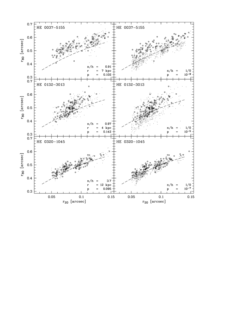
Figure 13: Comparison of observed data and model predictions. Observed quasar images are marked by circles, simulated data with dots. The panels on the left show the results for our ‘best guess’ models, with host galaxy fluxes and half-light radii as specified. For comparison, the right-hand panels refer to the ‘null hypothesis’ models having zero host galaxy flux.

Table 2: Two-dimensional KS test probabilities for a set of models with different host galaxy sizes, as well as for the null hypothesis of zero host galaxy flux. Bold numbers indicate the models with the highest probabilities.

		$r_{1/2}/$[kpc]								null
Object		1	2	4	7	12	20	35	60
	n/h		0.25	0.50	0.91	1.2	1.2	1.4	1.4	1/0
HE $0037-5155$	$K^{\mathrm{host}}$		15.6	15.8	16.1	16.2	16.2	16.3	16.3
	$p$		0.004	0.015	0.102	0.049	0.036	0.025	0.019	$3.6\leavevmode\nobreak\ 10^{-9}$
	n/h	0.17	0.83	0.97	1.7	2.6	2.9	3.2	3.2	1/0
HE $0132-3013$	$K^{\mathrm{host}}$	16.0	16.5	16.6	16.9	17.2	17.4	17.4	17.4
	$p$	7 $10^{-5}$	0.008	0.142	0.084	0.036	0.028	0.008	0.001	$2.1\leavevmode\nobreak\ 10^{-5}$
	n/h	1.5	2.2	3.1	3.6	3.7	3.7	3.8	4.0	1/0
HE $0320-1045$	$K^{\mathrm{host}}$	15.8	16.0	16.3	16.4	16.5	16.5	16.5	16.5
	$p$	0.004	0.007	0.022	0.033	0.095	0.056	0.049	0.043	$4.1\leavevmode\nobreak\ 10^{-7}$

In Fig. 13 we show observed and predicted distributions of $r_{20}$ vs. $r_{80}$ values for our three quasars. Each quasar is featured twice: In the right-hand panels we adopted the null hypothesis that no host galaxy is actually detected. It is immediately apparent that the observed and predicted distributions do not match at all. This is confirmed by applying the two-dimensional KS test (Peacock 1983) which yields $p\la 0.0001$ in all three cases. We conclude that an additional component is required in all of our quasars, with high significance. Notice that the relevant quantity is the distance along the displacement tracks of Fig. 10 (and not the proximity to the PSF tracks). Furthermore, while the rejection of the pure PSF model is significant even in moderate seeing conditions, any attempt to constrain the host galaxy size and hence the n/h ratio will fail without data in the best seeing regime (cf. Fig 8).

We now demonstrate that assuming the presence of quasar host galaxies with plausible physical parameters provides a statistically acceptable explanation for these extra components. The left-hand panels of Fig. 13 show the predictions of our ‘best guess’ models, compared again to the observed data. Notice that the selection of PSF stars according to a matched $r_{20,\mathrm{red}}$ distribution as illustrated in Fig. 11 ensures that even gaps in the observed distribution (such as those apparent in the top and bottom panels) are correctly taken into account.

There is no obvious mismatch between the observed and predicted points, for neither of the quasars. While some of the finer details may not be reproduced fully by the model, the overall degree of coincidence is satisfactory. A similar conclusion is reached by looking at the two-dimensional KS test, which gives acceptance probabilities of around 10–14 % for these models (see Table 2). While this is not exactly a high probability, it is above the conventional threshold of 5 % corresponding to a 2$\sigma$ confidence level. We therefore confirm that the image properties can be consistently described with the superposition of a nuclear point source plus an extended elliptical host galaxy.

Strictly speaking, this sort of consistency between model prediction and observations is all that the KS test can provide. It is generally not useful as a fitting tool, because of the discrete jumps of the KS diagnostic under continuous parameter variation. We have therefore just considered a very coarse grid of models, distinguished by different effective host galaxy radii, and subjected these to the two-dimensional KS test as described above. Results are also summarised in Table 2. We find again that very compact host galaxies compare poorly with the data; in one case (HE $0037-5155$) the offset between data points and the PSF track is so substantial that we could not even find a ‘best guess’ model for the smallest host galaxy model. But now also the most extended models show a significant decrease in their KS probabilities, due to the increased predicted scatter as explained above. Nevertheless we stress that the purpose of this exercise was not to determine a ’best-fit’ solution, but just to explore the range of models that are still compatible with the data. Table 3 summarises the results for one representative intermediate model of each quasar (which one might call our ‘best guess’), and provides relevant astrophysical parameters connected to each model.

Because of the degeneracy between effective radius and nuclear flux to host galaxy flux ratio n/h, the uncertainties in the size estimation translate directly into n/h uncertainties. In Table 2 we provide, for each assumed galaxy size, the corresponding n/h value and the apparent magnitude of the host galaxy. For the two quasars with fainter nuclei HE 0037$-$5155 and HE 0132$-$3013, the n/h depends strongly on galaxy size, while the uncertainty of n/h in the very bright object HE 0320$-$1045 is much less. As our procedure does not generate formal 1$\sigma$ errors, we simply adopt an uncertainty in effective radius of a factor of $\sim 2$ for the former two objects, and of a factor of $\sim 3$ for the latter, and we then estimate corresponding errors for the host galaxy fluxes. These are also listed in Table 3.

Table 3: Results of the analysis, for our ‘best guess’ model of each quasar host galaxy. n/h is the flux ratio between nucleus and host; $r_{50}$ is the half-light radius of the host galaxy along with the assumed range of possible values; $K_{\mathrm{nuc}}$ and $K_{\mathrm{host}}$ are the nucleus and host apparent $K_{s}$ band magnitudes at the ‘best guess’ and most extreme points in the range of $r_{50}$ values; $M_{R}^{\mathrm{nuc}}$ and $M_{R}^{\mathrm{host}}$ are the nuclear and host absolute magnitudes in the rest-frame $R$ band; $L/L_{\mathrm{Edd}}$ is the nuclear luminosity in multiples of the Eddington luminosity.

Name	n/h	$r_{50}$ [kpc]	$K^{\mathrm{nuc}}$	$K^{\mathrm{host}}$	$M_{R}^{\mathrm{nuc}}$	$M_{R}^{\mathrm{host}}$	$L/L_{\mathrm{Edd}}$
HE $0037-5155$	0.9	$7\pm$ 0.3 dex	$16.2^{+0.4}_{-0.1}$	$16.1^{+0.2}_{-0.3}$	$-27.1$	$-27.2$	0.1
HE $0132-3013$	1.0	$4\pm$ 0.3 dex	$16.6^{+0.1}_{-0.3}$	$16.6^{+0.3}_{-0.1}$	$-26.8$	$-26.9$	0.1
HE $0320-1045$	3.7	$12\pm$ 0.5 dex	$15.0^{+0.04}_{-0.01}$	$16.5^{+0.04}_{-0.1}$	$-28.5$	$-27.0$	0.6

Figure 14: Coadded images, based on the procedure described in the text. The left hand panels show azimuthally averaged surface brightness profiles of the quasar data (dots), the two scaled and coadded PSFs (dotted lines in red and black), and the remaining host galaxy images after subtraction of the different PSFs (solid lines). The middle panels show the quasar after PSF subtraction, both as contour and as a grayscale plot. The contours run at 1 mag/$\Box^{\prime\prime}$ spacing. The lowest isophote is 20 mag/$\Box^{\prime\prime}$. The red and black contours indicate the two different PSFs used. The right-hand panels show grayscale images of the residuals after subtracting the two PSF from each other. For colour versions of these figure see the online edition of the journal.

We finally computed high S/N images of each quasar by coadding only the images with $r_{20}$ below the median, i.e. the 50 % with the best observing conditions. To approximate a composite PSF for the combined images, we coadded only those stellar images that had been selected to represent the $r_{20}$ distribution of the quasar images (e.g. for HE 0320$-$1045 we took the stars contributing to the dashed histogram in Fig. 11 and inside the limits of the hashed bar). In order to ensure that the composition of a particular PSF had no influence on the final PSF image, we randomly split this set of images into two statistically independent subsets (PSF₁ and PSF₂), i.e. each PSF image contributes to only one final PSF. These PSF images were scaled to the quasar nuclear flux and subtracted. In Fig. 14 we show surface brightness profiles and contour plots of the coadded images, as well as the residuals after subtracting the two PSF images from each other. The two PSF images hardly differ at all, resulting in almost indistinguishable profiles and a residual which is confined to only the very central parts. The total flux of the PSF residual is zero, and the scatter around this value is less than 2 % of the original flux per pixel. Consequently, the two host galaxy images resulting from subtraction of the two PSFs are almost identical, which can clearly be seen in both the profile and the contour plots. From this we conclude that any structure detected in the host galaxy images is physical and not an artefact of the PSF subtraction.

6 Discussion

We have successfully detected the host galaxies underlying all of our three observed quasars. Resulting magnitudes and scale lengths are presented in Table 3. Since the rest-frame $R$ band is virtually identical with the observed $K$ band for all our objects, we neglected any K-corrections except the $(1+z)$ bandwidth term in computing the absolute magnitudes.

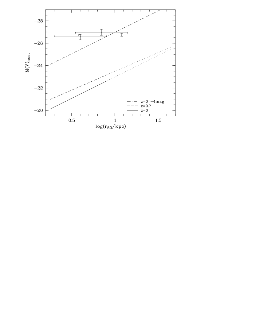
Figure 15: Luminosity-size relation of our three host galaxies (symbols), compared to literature relations. For ease of comparison, the $M_{R}$ magnitudes were converted to $M_{V}$ band assuming a rest-frame colour $V-R=0.27\pm 0.1$, appropriate for a single stellar population of intermediate age (100 Myr to 1 Gyr, based on solar metallicity models by Bruzual & Charlot 2003). The solid line is the relation for early type galaxies at $z\simeq 0$ from Shen et al. (2003) in the version given by McIntosh et al. (2005). The dashed line is the same relation for early type galaxies at $z\sim 0.7$ from GEMS (McIntosh et al. 2005). The dot-dashed line is the $z=0$ relation shifted by $-$4 mag. Dotted lines mark the extrapolation of the relations beyond the region covered by data.

These host galaxies are intriguingly luminous, especially given their relatively moderate sizes. In Figure 15 we relate these two quantities. Compared with empirical $M_{V}$-$r_{50}$ relations of early-type galaxies established at lower redshifts, our hosts are overluminous by at at least $\sim 4$ mag. If our hosts are roughly ellipticals, then they should have a much lower mass-to-light ratio than inactive elliptical galaxies at low redshifts, suggestive of a substantial young stellar population. It is difficult to quantify this in the absence of colour information, but if we simply assume that these galaxies will fade passively to reach the luminosity-size relations at low $z$, they would need to fade by $\sim 3.5$ mag within the next 4.2 Gyrs to $z=0.7$, or by $\sim 4$ mag within 10.5 Gyrs to $z=0$. A single stellar population of 100–150 Myr (solar metallicity; Bruzual & Charlot 2003) would have this property, fading by $\sim$3.2 mag and $\sim$4.0 mag in 4.2 Gyr and 10.5 Gyrs, respectively. Although this involves a lot of assumptions, the conclusion that we have detected the signature of a significant young stellar population is consistent with recent results from GEMS (Jahnke et al. 2004b) where similar ages were found for AGN hosts at $1.8<z<2.5$.

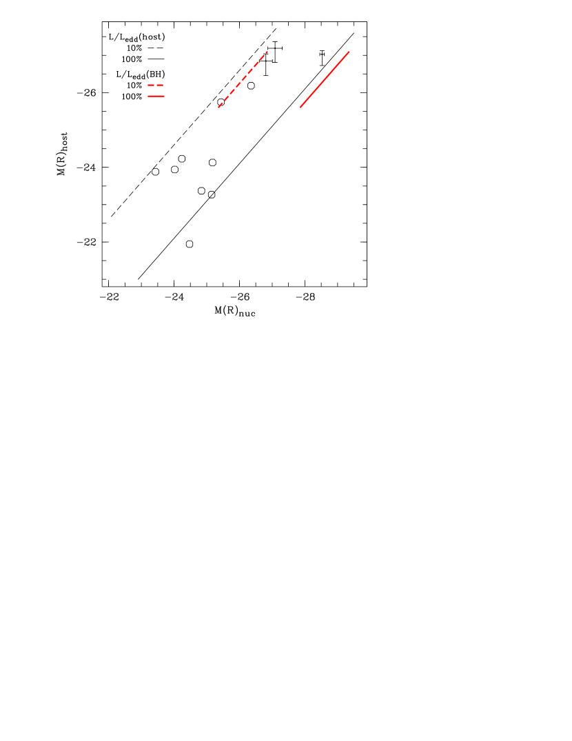
Figure 16: Nuclear versus host luminosities. Dots with error bars mark our data, circles mark hosts from the $z\sim 2$ sample of Kukula et al. (2001). We also plot lines of constant Eddington ratio derived from the host galaxy luminosities, extrapolated from low $z$ by assuming only passive evolution (thin black lines). The short thick-lines segments denote Eddington ratios derived from the spectroscopic black hole masses of our objects.

In Fig. 16 we plot nuclear luminosities against host luminosities for our objects. We also include the $z\sim 2$ results of Kukula et al. (2001), transformed to the rest-frame $R$ band assuming $(V-R)_{nuc}=0.4$, and zeropointing to the Vega system. This type of diagram has very often been constructed for quasar host galaxies at lower redshifts, showing clearly a correlation between quasar nuclear and host galaxy absolute magnitudes (McLeod & Rieke 1995). McLeod et al. (1999) demonstrated that this correlation is due to a physically motivated diagonal in this diagram, below and right of which there are no quasars because they would exceed their respective Eddington limits. In drawing this line, one has to assume a relation between host galaxy (spheroid or bulge) luminosity and the mass of the central black hole. While at low redshifts such a relation now seems well established (McLure & Dunlop 2002; Marconi & Hunt 2003; Häring & Rix 2004), it is by no means clear how a corresponding relation at $z\sim 2$ should look like. As a naive first guess we assumed that the same relation holds as at low redshifts, taking into account only passive evolution for a formation epoch at $z=3$. This is shown by the thin lines in Fig. 16 which mark the loci of quasars radiating at 10 % and 100 % of their Eddington luminosities.

Our quasars have nuclear absolute magnitudes that are on average $\sim 3$ mag brighter than those of Kukula et al. (2001). If the above correlation between nuclear and host luminosities pertains at these redshifts, our host galaxy luminosities should be brighter by a similar amount. This is indeed the case; our three datapoints form a seamless continuation of the Kukula et al. (2001) results, roughly along a diagonal line through the diagram. This implies that while our quasars have indeed very luminous host galaxies, they are not excessively luminous and fit well into the context of existing data.

So far, this does not mean that the McLeod et al. (1999) relation still holds at high redshifts, as the black hole masses in our quasars are essentially unknown and need not be coupled to the host galaxy luminosities as assumed above. However, recent work has opened an avenue to estimate, at least roughly, black hole masses using the width of the C iv emission line together with the continuum flux. The underlying assumption is that the motion of the line-emitting gas is virialized and that continuum flux and emission line width are estimators for the radius and the Keplerian velocity of the broad line region. A relation between $M_{\mathrm{BH}}$, the H$\beta$ line width and the optical continuum flux is established (e.g. Wandel et al. 1999; Kaspi et al. 2000) and has recently been extended to Mg ii (McLure & Jarvis 2002) and C iv (Vestergaard 2002). We have used the formula from the latter paper,

$$M_{\mathrm{BH}}=1.6\times 10^{6}\left[\frac{\mathrm{FWHM(C\>{\mbox{\sc iv}})}}{1000\mathrm{\>km\>s^{-1}}}\right]^{2}\left[\frac{\lambda L_{\lambda}(1350\>\mathrm{\AA})}{10^{44}\mathrm{\>ergs\>s^{-1}}}\right]^{0.7}$$ (2)

to predict virial black hole mass estimates for our quasars, using the spectra shown in Fig. 1. Results are summarised in Table 4. The approach has certainly large intrinsic uncertainties due to the unknown individual geometry and radiation anisotropy. Individual masses are probably not better determined than to $\pm 0.5$ dex, but unless the method is heavily biased, sample averages can be quite useful. For our small sample, we obtain a mean black hole mass of $3\times 10^{9}\>M_{\odot}$, with an uncertainty of at least 0.3 dex. These masses are consistent with predictions from low- to intermediate-redshift results (McLure & Dunlop 2002) as well as with actual high-redshift data (McLure & Dunlop 2003).

Table 4: Emission line widths of C IV and continuum fluxes at 1350 Å, together with the estimated black hole masses.

Object	${\scriptstyle\mathrm{FWHM}\atop\scriptstyle\mathrm{\>km\>s^{-1}}}$	$\log\left(\frac{\scriptstyle\lambda L_{\lambda}}{\scriptstyle\mathrm{\>ergs\>s^{-1}}}\right)$	$\log\left(\frac{\scriptstyle M_{\mathrm{BH}}}{\scriptstyle M_{\odot}}\right)$
HE $0037-5155$	5800	46.7	9.7
HE $0108-5952$	6000	46.3	9.4
HE $0132-3013$	5000	46.6	9.5
HE $0320-1045$	3300	47.1	9.4
HE $0418-0619$	6200	46.3	9.4

We now can compare each quasar absolute magnitude to its black hole mass and derive the Eddington ratio $L_{\mathrm{nuc}}/L_{\mathrm{Edd}}$, assuming mean quasar bolometric corrections taken from Elvis et al. (1994). Comparing these Eddington ratios with those obtained from the host galaxy luminosities we find that these are in very good agreement. For illustration, we have used the spectroscopically constrained Eddington ratios to predict where a quasar radiating at 100 % and at 10 % Eddington would be located in Fig. 16 (short thick lines). These line segments are displaced by less than a factor of 2 relative to the thin lines based on extrapolating the low-redshift relation, well within the uncertainties of our estimates. At least for our small set of very high luminosity quasars, these results are consistent with the notion that their host galaxies and black holes follow essentially the same relation as their present-day equivalents.

There is, however, a caveat to this statement. It implicitly assumes that our host luminosities are entirely due to stellar light from a homogeneous, well behaved stellar population. We now consider some possibilities that could devalidate this assumption.

A first effect could be the contamination by emission lines. While this is usually avoided by judiciously selecting the quasar sample such that no emission lines fall inside the filter regions, the very tight requirements of the AO system made it impossible for us to restrict the sample to redshift bins free of emission lines. In particular, H$\alpha$ lies perfectly inside the filter profile for all of our objects. Any extended H$\alpha$ contribution would lead to a corresponding reduction of the stellar light inside the $K$ band. Basically, there are three possible origins for extended H$\alpha$ emission: A large extended emission line region (EELR) powered by the quasar; H ii regions excited by young stars; or scattered light from the quasar nucleus. The last option can probably be dismissed, since the scattered H$\alpha$ flux in radio galaxies at $z\sim 1$ has been shown to be $\leq 10$ % of the nuclear flux (Leyshon & Eales 1998; Rigler et al. 1992). Assuming a scattered nuclear light fraction of this order results in a negligible contribution to the host galaxy magnitude for the objects having n/h $<1$. In the case of HE 0320$-$1045 the strength of the nuclear emission could contribute to the extended flux, though the actual amount of scattered flux cannot be quantified without access to colour information.

Moorwood et al. (2000) investigated a sample of $z\sim 2.2$ H$\alpha$-emitting galaxies and found that $L_{\mathrm{H}\alpha}/L_{K}\approx 1/5$ where $L_{K}$ is the luminosity of the galaxy in the $K$ band. If these results are portable to our quasar host galaxies (which is not unreasonable, see Vílchez & Iglesias-Páramo 1998), line emission from star-forming regions may increase the host galaxy luminosity by up to 0.2 magnitudes. A similar contribution of up to 0.1 magnitudes of H$\alpha$ to the $R$ band flux was found for low redshift quasar host galaxies (Jahnke et al. 2004a), in this case including possible EELR contributions.

Another significant contamination to the host galaxy luminosity could come from close companions. In other studies of host galaxies at high redshift this is a relatively common feature, and $\sim 40$ % of the objects analysed by Lehnert et al. (1999), Ridgway et al. (2001), Hutchings (1995), Sánchez et al. (2004), and Jahnke et al. (2004b) show companions. Since the effective field size used here is only $6\aas@@fstack{\prime\prime}4\times 6\aas@@fstack{\prime\prime}4$ due to the chopping between quadrants, no conclusions can be drawn on the density of field galaxies in the vicinity of our objects. However, in the direct images (Fig. 14) we see no signs of foreground galaxies or companions for two of the quasars, and their host galaxies appear quite round and undisturbed. HE 0320$-$1045, on the other hand, shows two extended features at $\sim 10$ kpc separation to the NE and SE of the nucleus which contain $\sim 50$ % of the host galaxy flux inside an aperture of 0$\aas@@fstack{\prime\prime}$6. In combination with the very pronounced core in the host galaxy luminosity profile (solid line in Fig. 14), this clearly indicates a host galaxy which is disturbed, accompanied by other galaxies or in the process of merging.

We conclude that the cumulative effect of all these mechanisms cannot be large, probably below 0.5 mag. The origin of the high luminosities of our quasar host galaxies must therefore be light from stars. We have shown that there is evidence for a relatively low mass-to-light ratio in these systems, and most of the rest-frame optical light in these quasar hosts could originate in young stars. Without colour information, however, we have no handle on estimating even rough stellar population properties. With4–12 kpc, the sizes of these objects fall within the range of 3–20 kpc found for less luminous quasar hosts at only slightly lower redshifts by Ridgway et al. (2001), Falomo et al. (2001) and Falomo et al. (2004). Given their sizes, these galaxies are clearly much more luminous than elliptical galaxies and QSO hosts at $z\simeq 0$ following the Kormendy (1977) relation (e.g. McLure et al. 1999). Further and more accurate measurements will be needed to quantitatively constrain the colours and sizes of such systems at high redshifts.

7 Conclusions

We have detected the host galaxies underlying three highly luminous $z\sim 2.2$ quasars, using near-infrared adaptive optics observations. We could estimate nuclear and host galaxy luminosities as well as constrain their sizes, but there is some degeneracy between these parameters. The measured host luminosities are among the highest yet measured at these redshifts, but the quasars are also among the most luminous to be resolved. Our measurements are in good agreement with other results obtained for similar redshifts, and the location of the host galaxies in a $L_{\mathrm{nuc}}$ vs. $L_{\mathrm{host}}$ diagram suggests that the quasars radiate at roughly 10–50 % of their Eddington luminosities, similar to low-redshift quasars. Comparing our results to the magnitude-size relation at $z=0$ and $z=0.7$ indicates a much lower mass-to-light ratio in the host galaxies than for an old population. A dominating stellar population of 100–150 Myrs age would have a passive fading to allow an evolution of our host galaxies onto the lower redshift magnitude-size relation.

In getting these results, we have both taken advantage of, and suffered from the special conditions occurring when working with adaptive optics. The capability of measuring the scale length of a $z\sim 2$ galaxy in the presence of a bright nucleus is certainly owned to the high angular resolution achieved, especially as our quasar hosts appear to be rather compact. On the other hand, we had to overcome several difficulties caused by the strong dependence of the image quality on the actual atmospheric conditions.

Careful determination of the PSF is a condition without exception for the analysis of host galaxies of luminous quasars. For AO observations this usually poses a big problem, because of the generally small field of view and the strong field anisoplanatism. We have described a conceptually simple procedure that enabled us to incorporate non-simultaneously observed PSF stars in a straightforward manner, even though the image quality varied substantially during the observing sessions.

While the performance of current AO instruments has certainly improved dramatically compared to the relatively ancient system that we used, some of the problems mentioned above are still the same. Detectors have become larger, but since larger telescopes require smaller pixels in order to sample the PSF core adequately, the field of view has not necessarily grown in proportion. This means that also in the future, quasars with a suitable PSF star in the same field of view and the same degree of field anisoplanatism will be very rare; thus, non-simultaneous PSF observations will often be necessary also in the future. One of the objectives of this paper is to create awareness that non-optimal atmospheric conditions do exist, and that one needs to account for rapid variability of observing conditions on all time scales. In this sense, AO observations are much more difficult to handle than normal seeing-limited imaging. Indeed, near-infrared imaging under good seeing conditions is probably at least competitive to AO as long as mere detections of high-redshift quasar hosts are sought. On the other hand, AO data provide insights into quasar host structural properties on kpc scales. In this domain, AO observations will be unbeatable from the ground, and further development of specific analysis tools will be well worth the effort.