Speeding Up Cosmological Boltzmann Codes

Abstract

We introduce a novel strategy for cosmological Boltzmann codes leading to an increase in speed by a factor of $\sim 30$ for small scale Fourier modes. We (re-)investigate the tight coupling approximation and obtain analytic formulae including the octupoles of photon intensity and polarization. Numerically, these results reach optimal precision. Damping rapid oscillations of small scale modes at later times, we simplify the integration of cosmological perturbations. We obtain analytic expressions for the photon density contrast and velocity as well as an estimate of the quadrupole from after last scattering until today. These analytic formulae hold well during re-ionization and are in fact negligible for realistic cosmological scenarios. However, they do extend the validity of our approach to models with very large optical depth to the last scattering surface.

I Introduction

Standard codes such as cmbfast Seljak:1996is ; cmbfast , camb Lewis:1999bs ; Lewis:2002ah ; camb or cmbeasy Doran:2003sy ; Doran:2003ua ; cmbeasy compute the evolution of small perturbations in a Friedman-Robertson-Walker Universe. The output most frequently used are multipole spectra of the Cosmic Microwave Background (CMB) and power spectra of massive particles. These predictions are compared to precision measurements of the Cosmic Microwave Background (CMB) Spergel:2003cb and Large Scale Structure (LSS) Tegmark:2003ud . Working in Fourier space, the codes evolve perturbation equations for single Fourier $k$-modes. The simulated evolution starts well outside the horizon at early times and ends today. For the CMB, relevant scales lie in the range $k\sim 10^{-5}\dots 1\,\textrm{Mpc}^{-1}$, while those for the LSS extend to higher $k\sim 5\dots 1000\,\textrm{Mpc}^{-1}$.

Currently, the time needed to evolve a single mode is roughly proportional to $k$. As the spectrum is computed in logarithmic $k$-steps, the largest few $k$-modes tend to dominate the resources needed for the entire calculation. We have analyzed the current strategy to integrate the perturbation equations and singled out two bottlenecks. The first one is the so called tight coupling regime (or better: the end of tight coupling). The second one are rapid oscillations of relativistic quantities for high $k$-modes. Roughly speaking, in standard cmbfast and cmbeasy, both regimes contribute equally to the computational cost. This is likely not the case for camb, as it uses a higher order scheme during tight coupling – a solution similar to the one we will present later on.

Figure 1: The CMB multipole spectrum up to $l=4000$ for a standard cosmological model (solid line). The dashed (blue) line shows the relative deviation between a standard cmbeasy calculation and one where the switch ending tight coupling has been pushed to earlier times and hence better precision. The geometric average deviation is $\sim 0.3\%$. The dashed-dotted (red) line shows the deviation between such a high precision cmbeasy calculation and the new algorithm. With the average geometric deviation $\sim 0.01\%$ roughly 30 times smaller, our new algorithm comes close to the optimal result.

Our strategy therefore consists of two parts. The first one is a revised tight coupling treatment. In this, we will make a conceptual change, distinguishing between tight coupling of the baryon and photon fluid velocities on one hand and the validity of an analytic treatment of the photon intensity and polarization quadrupole on the other. In essence, our solution extends to the octupole. We thus capture the physics during tight coupling better than previously achieved. This leads to a considerable increase in accuracy reaching the optimal precision for this stage of the computation (see Figure 1).

The second part of our solution consists of suppressing unwanted oscillations in the multipole components of relativistic particles. In essence, it is the line-of-sight Seljak:1996is formulation of all modern CMB codes that allows us to do this. As we will see, the oscillations we suppress are anyhow unphysical as they perpetuate unwanted reflections due to truncation effects. In any case, the modifications are such that observational quantities like the CMB or LSS are not influenced by our choice. These two improvements combined lead to considerably shorter integration times. Typically, the benefit sets in for modes $k\gtrapprox 0.1\,\textrm{Mpc}^{-1}$ and increases gradually until reaching factors of $\sim 30$ for modes $\sim 5\,\textrm{Mpc}^{-1}$ and higher. For some speed comparisons, see Table 1.

$k_{max}/h$	$l_{max}$	cmbeasy	cmbeasy
		(new algorithm)	(sync. gauge)
$10\,\textrm{Mpc}^{-1}$	no CMB	1.5s	10s
$100\,\textrm{Mpc}^{-1}$	no CMB	4s	93s
$5\,\textrm{Mpc}^{-1}$	2000	5s	12s
$10\,\textrm{Mpc}^{-1}$	4000	9s	25s

Table 1: Comparison of speed between the new algorithm and the standard synchronous gauge implementation. Execution times of cmbfast are comparable to the standard synchronous gauge implementation, but can deviate by a factor of $\sim\frac{1}{2}\dots 2$ from cmbeasy depending on the task. The Hubble parameter for the model used was $h=0.7$.

II Tight coupling revised

At early times, the photon and baryon fluids are strongly coupled via Thomson scattering. The mean free path between collisions of a photon $\tau_{c}^{-1}\equiv an_{e}\sigma_{T}$ is given in terms of the number density of free electrons $n_{e}$, the scale factor of the Universe $a$ and Thomson cross section $\sigma_{T}$. During early times, Hydrogen and Helium are fully ionized, hence $n_{e}\propto a^{-3}$ and $\tau_{c}\propto a^{2}$. During Helium and Hydrogen recombination, this scaling argument does not hold (see Figure 2). To avoid these periods we resort to the correct value of $\dot{\tau}_{c}$ computed beforehand instead of using $\dot{\tau}_{c}=2\frac{\dot{a}}{a}\tau_{c}$ for redshifts $z<10^{4}$. The effect of assuming that the scaling holds would however be considerably less than $1\%$ on the final CMB spectrum.

To discuss the tight coupling regime, let us recapitulate the evolution equations for baryons and photons. We do this in terms of their density perturbation $\delta$ and bulk velocity $v$. For photons, we additionally consider the shear $\sigma_{\gamma}$ and higher multipole moments $\mathcal{M}_{l}$ of the intensity as well as polarization multipoles $E_{l}$. Our variables are related to the ones of Ma:1995ey by substituting $v\to k^{-1}\theta$. In longitudinal gauge, baryons evolve according to

$$\dot{\delta}_{b} = -kv_{b}+3\dot{\phi}$$ (1)

$$\dot{v}_{b} = -\frac{\dot{a}}{a}v_{b}+c_{s}^{2}k\delta_{b}+R\tau_{c}^{-1}(v_{\gamma}-v_{b})+k\psi,$$ (2)

where $R\equiv(4/3)\rho_{\gamma}/\rho_{b}$, the speed of sound of the baryons is denoted by $c_{s}^{2}$ and $\phi$ and $\psi$ are metric perturbations. By definition, $R\propto a^{-1}$ (provided no baryons are converted to other forms of energy) and at the time of interest, $c_{s}^{2}\propto T_{b}=T_{\gamma}\propto a^{-1}$ (for more detail see e.g. Ma:1995ey ). Photons evolve according to the hierarchy

$$\dot{\delta}_{\gamma} = -\frac{4}{3}kv_{\gamma}+4\dot{\phi}$$ (3)

$$\dot{v}_{\gamma} = k\left(\frac{1}{4}\delta_{\gamma}-\sigma_{\gamma}\right)+k\psi+\tau_{c}^{-1}(v_{b}-v_{\gamma}),$$ (4)

$$\frac{5}{2}\dot{\sigma}_{\gamma} = \dot{\mathcal{M}}_{2}=-\tau_{c}^{-1}\left(\frac{9}{10}\mathcal{M}_{2}+\frac{\sqrt{6}}{10}E_{2}\right)$$ (5)

$$\hskip 71.13188pt+k\left(\frac{2}{3}v_{\gamma}-\frac{3}{7}\mathcal{M}_{3}\right)$$

$$\dot{\mathcal{M}}_{l} = k\!\left(\frac{l}{2l-1}\mathcal{M}_{l-1}\!-\!\frac{l+1}{2l+3}\mathcal{M}_{l+1}\right)\!-\!\tau_{c}^{-1}\mathcal{M}_{l},$$ (6)

where the $E$-type polarization obeys

$$\dot{E}_{2} = -k\frac{\sqrt{5}}{7}E_{3}-\tau_{c}^{-1}\left(\frac{4}{10}E_{2}+\frac{\sqrt{6}}{10}M_{2}\right)$$ (7)

$$\dot{E}_{l} = -\tau_{c}^{-1}E_{l}$$ (8)

$$\ \ +k\left(\frac{\sqrt{l^{2}-4}}{2l-1}E_{l-1}-\frac{\sqrt{l^{2}+2l-3}}{2l+3}E_{l+1}\right).$$

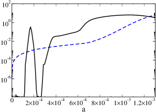
Figure 2: Relative deviation of $\dot{\tau}_{c}$ from the naive scaling relation: $[\dot{\tau}_{c}-2(\dot{a}/a)\tau_{c}]/[2(\dot{a}/a)\tau_{c}]$ (solid line). We also depict the product $\tau_{c}\frac{\dot{a}}{a}$ (dashed line) vs. the scale factor $a$, which compares the mean free path to the expansion rate of the Universe. In the cosmological model used, matter radiation equality is at $a_{equ}=3\times 10^{-4}$ and last scattering defined by the peak of the visibility function is at $a_{ls}=9\times 10^{-4}$. The deviation around $a=2\times 10^{-4}$ is from Helium recombination and is practically negligible, because the visibility is still small during that period. At later times, however the deviation is due to the onset of Hydrogen recombination and takes on substantial values before last scattering.

The overwhelmingly large value of $\tau_{c}^{-1}$ precludes a straight forward numerical integration at early times: tiny errors in the propagation of $v_{b}$ and $v_{\gamma}$ lead to strong restoring forces. This severely limits the maximum step size of the integrator and hence the speed of integration. Ever since Peebles and Yu Peebles:ag first calculated the CMB fluctuations, one resorts to the so called tight coupling approximation. This approximation eliminates all terms of order $\tau_{c}^{-1}$ from the evolution equations assuming tight coupling at initial times. Our discussion will closely lean on that of Ma:1995ey , taking a slightly different route. In contrast to Ma:1995ey , however, we will keep all terms in the derivation. Like Ma:1995ey , we start by solving (4) for $(v_{b}-v_{\gamma})$ and write $\dot{v}_{\gamma}=\dot{v}_{b}+(\dot{v}_{\gamma}-\dot{v}_{b})$ to get Equation (71) of Ma:1995ey

$$(v_{b}-v_{\gamma})=\tau_{c}\left[\dot{v}_{b}+(\dot{v}_{\gamma}-\dot{v}_{b})-k\left(\frac{1}{4}\delta_{\gamma}-\sigma_{\gamma}+\psi\right)\right].$$ (9)

Substituting Equation (2) for $\dot{v}_{b}$ into this Equation (9), one gets Equation (72) of Ma:1995ey

$$\frac{(1+R)}{\tau_{c}}(v_{b}-v_{\gamma})=-\frac{\dot{a}}{a}v_{b}+(\dot{v}_{\gamma}-\dot{v}_{b})\\ +k\left(c_{s}^{2}\delta_{b}-\frac{1}{4}\delta_{\gamma}+\sigma_{\gamma}\right).$$ (10)

Deriving the LHS of this Equation (10) yields

$$\dot{\textrm{lhs}} = \frac{(1+R)}{\tau_{c}}(\dot{v}_{b}-\dot{v}_{\gamma})$$ (11)

$$\quad-(v_{b}-v_{\gamma})\left[\frac{\dot{a}}{a}\frac{R}{\tau_{c}}-\frac{1+R}{\tau_{c}}\frac{\dot{\tau}_{c}}{\tau_{c}}\right]$$

$$\overset{*}{=} \frac{(1+R)}{\tau_{c}}(\dot{v}_{b}-\dot{v}_{\gamma})-\frac{2+3R}{\tau_{c}}\frac{\dot{a}}{a}(v_{b}-v_{\gamma}),$$ (12)

where the last line holds provided the assumed scaling of $\tau_{c}$ is correct (see also Figure 2). All in all, deriving Equation (10) with respect to conformal time yields

$$\frac{(1+R)}{\tau_{c}}(\dot{v}_{b}-\dot{v}_{\gamma})-\left[\frac{\dot{a}}{a}\frac{R}{\tau_{c}}-\frac{1+R}{\tau_{c}}\frac{\dot{\tau}_{c}}{\tau_{c}}\right](v_{b}-v_{\gamma})\\ =(\ddot{v}_{\gamma}-\ddot{v}_{b})-\frac{\ddot{a}}{a}v_{b}+\left(\frac{\dot{a}}{a}\right)^{2}v_{b}-\frac{\dot{a}}{a}\dot{v}_{b}\\ +k\left(\dot{c}_{s}^{2}\delta_{b}+c_{s}^{2}\dot{\delta}_{b}-\frac{1}{4}\dot{\delta}_{\gamma}+\dot{\sigma}_{\gamma}\right)$$ (13)

Multiplying Equation (2) by $\frac{\dot{a}}{a}$ to substitute $\frac{\dot{a}}{a}\dot{v}_{b}$ in (13), we get

$$\frac{(1+R)}{\tau_{c}}(\dot{v}_{b}-\dot{v}_{\gamma})=\left[\frac{\dot{a}}{a}\frac{R}{\tau_{c}}-\frac{1+R}{\tau_{c}}\frac{\dot{\tau}_{c}}{\tau_{c}}\right](v_{b}-v_{\gamma})\\ +(\ddot{v}_{\gamma}-\ddot{v}_{b})-\frac{\ddot{a}}{a}v_{b}+2\left(\frac{\dot{a}}{a}\right)^{2}v_{b}-2\frac{\dot{a}}{a}c_{s}^{2}k\delta_{b}\\ +k\left(c_{s}^{2}\dot{\delta}_{b}-\frac{1}{4}\dot{\delta}_{\gamma}+\dot{\sigma}_{\gamma}\right)+\frac{\dot{a}}{a}k\psi$$ (14)

where we have used $\dot{c}_{s}^{2}=-\frac{\dot{a}}{a}c_{s}^{2}$. We could stop here, however it is numerically better conditioned to write $2\left(\frac{\dot{a}}{a}\right)^{2}v_{b}=2\frac{\dot{a}}{a}\left(\frac{\dot{a}}{a}v_{b}\right)$ where $\frac{\dot{a}}{a}v_{b}$ is obtained from solving Equation (10) for $\frac{\dot{a}}{a}v_{b}$. This expression for $\left(\frac{\dot{a}}{a}\right)^{2}v_{b}$ is then plugged into Equation (14) to yield the final result for the slip (denoted by $\mathcal{\dot{V}}$)

$$\mathcal{\dot{V}}\equiv(\dot{v}_{b}-\dot{v}_{\gamma})=\Bigg{\{}\left[\frac{\dot{\tau}_{c}}{\tau_{c}}-\frac{2}{1+R}\right]\frac{\dot{a}}{a}(v_{b}-v_{\gamma})\\ +\frac{\tau_{c}}{1+R}\bigg{[}-\frac{\ddot{a}}{a}v_{b}+(\ddot{v}_{\gamma}-\ddot{v}_{b})+k\left(\frac{1}{2}\delta_{\gamma}-2\sigma_{\gamma}+\psi\right)\\ +k\left(c_{s}^{2}\dot{\delta}_{b}-\frac{1}{4}\dot{\delta}_{\gamma}+\dot{\sigma}_{\gamma}\right)\bigg{]}\Bigg{\}}\Bigg{/}\left\{1+2\frac{\dot{a}}{a}\frac{\tau_{c}}{1+R}\right\}.$$ (15)

or alternatively, at times when the scaling of $\tau_{c}$ holds,

$$\mathcal{\dot{V}}\equiv(\dot{v}_{b}-\dot{v}_{\gamma})=\Bigg{\{}\frac{2R}{1+R}\frac{\dot{a}}{a}(v_{b}-v_{\gamma})\\ +\frac{\tau_{c}}{1+R}\bigg{[}-\frac{\ddot{a}}{a}v_{b}+(\ddot{v}_{\gamma}-\ddot{v}_{b})+k\left(\frac{1}{2}\delta_{\gamma}-2\sigma_{\gamma}+\psi\right)\\ +k\left(c_{s}^{2}\dot{\delta}_{b}-\frac{1}{4}\dot{\delta}_{\gamma}+\dot{\sigma}_{\gamma}\right)\bigg{]}\Bigg{\}}\Bigg{/}\left\{1+2\frac{\dot{a}}{a}\frac{\tau_{c}}{1+R}\right\}.$$ (16)

This Equation (15) (or more obviously (16)) is essentially Equation (74) of Ma:1995ey up to some corrections. Having kept all terms, we note that our Equation (15) is exact. To obtain Equations of motion for $v_{b}$ and $v_{\gamma}$ during tight coupling, we plug our result for $(\dot{v}_{b}-\dot{v}_{\gamma})$, Equation (15) into the RHS of Equation (9) and this in turn into the RHS of Equations (2) and (4). This yields

$$\dot{v}_{b} = \frac{1}{1+R}\left(kc_{s}^{2}\delta_{b}-\frac{\dot{a}}{a}v_{b}\right)+k\psi$$

$$\qquad\frac{R}{1+R}\left[k\left(\frac{1}{4}\delta_{\gamma}-\sigma_{\gamma}\right)+\mathcal{\dot{V}}\right]$$

$$\dot{v}_{\gamma} = \frac{R}{1+R}k\left(\frac{1}{4}\delta_{\gamma}-\sigma_{\gamma}\right)+k\psi$$ (17)

$$\qquad+\frac{1}{1+R}\left(kc_{s}^{2}\delta_{b}-\frac{\dot{a}}{a}v_{b}-\mathcal{\dot{V}}\right)$$

Up to now, we have made no approximations. Conceptually, we would like to separate the question of tight coupling for the velocities $v_{\gamma}$ and $v_{b}$ from any approximations of the shear $\sigma_{\gamma}$ which we make below. As far as the tight coupling of the velocities and hence the slip $\mathcal{\dot{V}}$ is concerned, our approximation is to drop the term $(\ddot{v}_{\gamma}-\ddot{v}_{b})$. We reserve the expression ’tight coupling’ for the validity of our assumption that $(\ddot{v}_{\gamma}-\ddot{v}_{b})$ can be neglected in the slip $\mathcal{\dot{V}}$. As a criterion, we use $k\tau_{c}<\frac{2}{10}$ for the photon fluid. When this threshold is passed, we use Equation (4) to evolve the photon velocity. Likewise, for the baryons, we use ${\rm max}(k,\frac{\dot{a}}{a})\tau_{c}/R<\frac{4}{100}$. Again, when this limit is exceeded, we switch to Equation (2). In any case, we switch off the approximation $\Delta\tau=30\,\textrm{Mpc}$ before the first evaluation of the CMB anisotropy sources (see below). For a $\Lambda-{\rm CDM}$ model, this is at $\tau\approx 200\,\textrm{Mpc}$.

To obtain high accuracy during tight coupling, it is crucial to determine $\sigma_{\gamma}$. Not so much for the slip (15), but more so for the Equations of motion (17): the shear reflects the power that is drained away from the velocity in the multipole expansion. This leads to an additional damping for photons. For the shear, we distinguish two regimes: an early one, where we use a high-order analytic approximation and a later one in which the full multipole equations of motion are used.

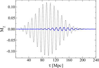
Figure 3: The quadrupole $\mathcal{M}_{2}$ obtained by a full numerical evolution for a mode of $k=1\,\textrm{Mpc}^{-1}$ (dotted line). The solid (blue) line depicts the deviation of our analytic result, Equation (21) from the numerical value. For this mode, we normally switch to the full numerical evolution at $\tau=65\,\textrm{Mpc}$ when the analytic estimate still holds very well.

Since $\tau_{c}\ll 1$ at early times, one gets from multiplying (6) by $\tau_{c}$ that $\mathcal{M}_{l}\approx\left(k\tau_{c}\right)\mathcal{M}_{l-1}l/(2l-1)$. Hence, higher multipoles are suppressed by powers of $k\tau_{c}$. Approximating this situation by $\dot{\mathcal{M}}_{3}=\dot{E}_{3}=\mathcal{M}_{4}=E_{4}=0$ in Equations (6) and (8), we get

$$\mathcal{M}_{3} = \frac{3}{5}\left(k\tau_{c}\right)\mathcal{M}_{2}$$

$$E_{3} = \frac{1}{\sqrt{5}}\left(k\tau_{c}\right)E_{2}.$$ (18)

Likewise, we obtain a leading order estimate of the quadrupoles by temporarily setting $\dot{\mathcal{M}}_{2}=\dot{E}_{2}=0$,

$$\frac{5}{2}\sigma_{\gamma}^{l.o.}=\mathcal{M}_{2}^{l.o.} = \frac{8}{9}\left(k\tau_{c}\right)v_{\gamma}$$ (19)

$$E_{2}^{l.o.} = -\frac{\sqrt{6}}{4}\mathcal{M}_{2}^{l.o.}.$$ (20)

Inserting Equations (18) into the quadrupole Equations (5) and (7) and using $\dot{\mathcal{M}}_{2}=\dot{\mathcal{M}}_{2}^{l.o.}$ and $\dot{E}_{2}=\dot{E}_{2}^{l.o.}$ as an estimate for the derivative, we get the desired expression for the shear

$$\frac{5}{2}\sigma_{\gamma}=\mathcal{M}_{2}=\frac{8}{9}k\tau_{c}v_{\gamma}\left[1-\frac{29}{70}\left(k\tau_{c}\right)^{2}\right]-\frac{11}{6}\tau_{c}\dot{\mathcal{M}}_{2}^{l.o.},$$ (21)

which is precise to order $\tau_{c}$ and $\left(k\tau_{c}\right)^{2}$ (see also Figure 3). The inclusion of the octupole reduces the power of $\mathcal{M}_{2}$ as expected.

In practice, we use $\mathcal{M}_{2}^{l.o.}$ to calculate the slip $\mathcal{\dot{V}}^{l.o}$ to leading order. This in turn is used to calculate $\dot{v}_{\gamma}^{l.o}$. From $\dot{v}_{\gamma}^{l.o}$, we get $\dot{\mathcal{M}}_{2}^{l.o.}$ which in turn is needed to obtain the accurate value of $\mathcal{M}_{2}$ according to Equation (21). The difference $\Delta\mathcal{M}_{2}\equiv\mathcal{M}_{2}-\mathcal{M}_{2}^{l.o.}$ is then used to promote $\mathcal{\dot{V}}^{l.o}\to\mathcal{\dot{V}}$ as well as $\dot{v}_{\gamma}^{l.o.}\to\dot{v}_{\gamma}$. Finally, having $\mathcal{M}_{2}$ and $\mathcal{\dot{V}}$ at hand, we get $\dot{v}_{b}$ from Equation (17).

When this approximation breaks down (sometimes long before tight coupling ends), we switch to the full multipole evolution equations. Tight coupling is applicable for $k\tau_{c}\ll 1$. Equation (21) on one hand goes to higher order in $k\tau_{c}$, namely, as $\mathcal{M}_{2}^{l.o.}$ is already of order $\left(k\tau_{c}\right)$, our results incorporates quantities up to $\left(k\tau_{c}\right)^{3}$. In terms of $\tau_{c}$ alone, however, Equation (21) is accurate to order $\tau_{c}\left(k\tau_{c}\right)$ only. Hence, when $\tau_{c}$ reaches $\sim 10^{-1}\,\textrm{Mpc}$, our analytic expression is not sufficiently accurate anymore. This signals the breakdown of our assumption that $\dot{\mathcal{M}}_{3}=\dot{E}_{3}=0$ (and likewise for higher multipoles). Luckily, it is not critical to evolve the full multipole equations even when $\tau_{c}^{-1}$ is still substantial. This is in strong contrast to the coupled velocity equations which are far more difficult to evolve at times when the analytic quadrupole formulae breaks down. In essence, distinguishing between tight coupling and the treatment of the quadrupole evolution is the key to success here.

III A Cure for Rapid Oscillations

While the gain in speed from the method described in the last section is impressive, high $k$-modes would still require long integration times. To see this, one must consider the evolution of the photon and neutrino multipole hierarchies. Our discussion is aimed at small scale modes which are supposed to be well inside the horizon, i.e. $k\tau\gg 1$.

Before last scattering, $\left(k\tau_{c}\right)\ll 1$ and $\mathcal{M}_{l}\propto\left(k\tau_{c}\right)^{l-1}$ for $l>1$ and so the influence of higher multipoles on $\delta_{\gamma}$ and $v_{\gamma}$ may be neglected to first order. In the small scale limit that we are interested in, $\delta_{\gamma}$ and $v_{\gamma}$ are oscillating according to $\delta_{\gamma}\sim\cos(c_{s}^{\gamma}k\tau)$ and $v_{b}\sim\sin(c_{s}^{\gamma}k\tau)$. As the speed of sound of the photon-baryon fluid is $c_{s}^{\gamma}\approx\sqrt{1/3}$, we encounter oscillations with period $\Delta\tau\approx(2\pi)/(kc_{s}^{\gamma})\approx 11/k$. Estimating the time of last scattering with $\tau_{ls}\approx 280\,\textrm{Mpc}$, we see that a mode will perform $\tau_{ls}/\Delta\tau\approx 25k\,\textrm{Mpc}$ oscillations until last scattering. Yet, there are many more oscillations after last scattering which we turn to now. After last scattering, $\tau_{c}^{-1}$ is negligible and the multipole hierarchy of photons effectively turns into recursion relations for spherical Bessel functions. The same is true for neutrino multipoles which roughly evolve like spherical Bessel functions from the start. Spherical Bessel functions have a leading order behavior similar to $j_{l}(k\tau)\propto(k\tau)^{-3/2}\sin(k\tau)$ for $k\tau\gg 1$ and $k\tau>l$. The period is then given by $\Delta\tau=(2\pi)/k$. The time passed from last scattering to today, is $\tau_{0}-\tau_{ls}\approx\tau_{0}\approx 14000\,\textrm{Mpc}$ for current cosmological models. So we encounter $\sim\tau_{0}/\Delta_{\tau}\approx k\tau_{0}/(2\pi)$ =$2200\times k\,\textrm{Mpc}$ oscillations. Numerically, each oscillation necessitates $\sim 20\dots 40$ evaluations of the full set of evolution equations. We therefore estimate a total of $\sim 6\times 10^{4}\times k\,\textrm{Mpc}$ evaluations induced by the oscillatory nature of the solution. So a mode $k=5\,\textrm{Mpc}^{-1}$ needs $\sim 3\times 10^{5}$ evaluations – a substantial number.

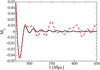
Figure 4: The quadrupole as a function of conformal time $\tau$ for a mode of $k/h=0.5\,\textrm{Mpc}^{-1}$ and $h=0.7$. The multipole expansion for photons and neutrinos has been truncated at $l_{max}=200$ (solid line) and $l_{max}=8$ (dashed line) respectively. In the case of $l_{max}=8$, power reflected back from the highest multipole $l_{max}$ renders the further evolution of the quadrupole unphysical. Indeed the magnitude of the physical oscillations are much smaller than the reflected ones. For $l_{max}=200$, reflection effects dominate the evolution from $\tau\sim 1300\,\textrm{Mpc}$ on. In both cases, the effect of shear of realistic particles on the potentials $\phi$ and $\psi$ is negligible by the time the truncation effects set in.

Since the introduction of the line-of-sight algorithm, what one really needs for the CMB and LSS are the low multipoles up to the quadrupoles. In fact, the sources for temperature and polarization anisotropies are given by

$$S_{T}=e^{\kappa(\tau)-\kappa(\tau_{0})}\left[\dot{\phi}+\dot{\psi}\right]+\dot{g}\left[\frac{v_{b}}{k}+\frac{3}{k^{2}}\dot{\mathcal{C}}\right]+\ddot{g}\frac{3}{2k^{2}}\mathcal{C}\\ +g\left[\frac{1}{4}\delta_{\gamma}+\frac{\dot{v}_{b}}{k}+(\phi+\psi)+\frac{\mathcal{C}}{2}+\frac{3}{2k^{2}}\ddot{\mathcal{C}}\right]$$ (22)

and

$$S_{E}=\frac{3\,g}{2}\mathcal{C}\,\left(k\left[\tau_{0}-\tau\right]\right)^{-2}$$ (23)

Here, $g\equiv\dot{\kappa}\exp(\kappa(\tau)-\kappa(\tau_{0}))$ is the visibility with $\dot{\kappa}\equiv\tau_{c}^{-1}$ the differential optical depth and $\mathcal{C}\equiv(\mathcal{M}_{2}-\sqrt{6}E_{2})/10$ contains the quadrupole information. The role of higher multipole moments is therefore reduced to draining power away from $\delta_{\gamma}$, $v_{\gamma}$ and $\mathcal{M}_{2}$ and $E_{2}$ (and likewise for neutrinos). As the oscillations are damped and tend to average out, it suffices to truncate the multipole hierarchy at low $l\sim 8\dots 25$ in the line-of-sight approach. This is one of the main reasons for its superior speed. Truncating the hierarchy, though leads to unwanted reflection of power from the highest multipole $l_{max}$. As one can see in Figure 4, the power reflected back spoils the mono frequency of the oscillations. At best, the further high frequency evolution of the multipoles is wrong but negligible, because the oscillations are small and average out. This is indeed the case in the cmbfast/camb/cmbeasy truncation.

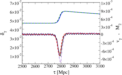
Figure 5: Photon density contrast $\delta_{\gamma}$ (upper solid [blue] line), $v_{\gamma}$ (lower solid [black] line) and quadrupole $\mathcal{M}_{2}\equiv(5/2)\sigma_{\gamma}$ (dashed dotted [indigo] line) as a function of conformal time $\tau$ before and after re-ionization at $\tau\approx 2800\,\textrm{Mpc}$. The [green] upper dashed line is the analytic estimate for $\delta_{\gamma}$, Equation (27) and the lower [red] dashed line is the analytic estimate for $v_{\gamma}$, Equation (28). The analytic estimate of $\delta_{\gamma}$ falls almost on top of the correct numerical result. Please note the different scales for $\delta_{\gamma}$ and $v_{\gamma}$ and $\mathcal{M}_{2}$ respectively. The quadrupole is roughly of the same order as $v_{\gamma}$. The mode shown is for $k/h=5\,\textrm{Mpc}^{-1}$ where $h=0.7$ and the optical depth to the last scattering surface is $\tau_{opt}=0.3$. Please note that we truncated the multipole hierarchy at sufficiently high $l_{max}=2500$. With insufficient $l_{max}$, rapid unphysical oscillations of considerably higher amplitude would be present.

We will now show that the overwhelming contribution from $\delta_{\gamma}$ and $\mathcal{C}$ (and its derivatives) of some small scale mode $k>10^{-1}\,\textrm{Mpc}^{-1}$ towards CMB fluctuations comes from times before re-ionization. To do this, let us find an analytic approximation to the photon evolution after decoupling and in particular during re-ionization. Without re-ionization, and neglecting $\mathcal{M}_{2}$ as well as using $\phi\approx\psi$ and $\ddot{\phi}\approx 0$, the equation of motions (3) and (4) can be cast in the form

$$\ddot{\delta}_{\gamma}=-\frac{4}{3}k^{2}\left(\frac{1}{4}\delta_{\gamma}+\psi\right),$$ (24)

which has the particular solution

$$\delta_{\gamma}=-4\psi.$$ (25)

As the oscillations of $v_{\gamma}$ and higher multipoles are damped roughly $\propto(k\tau)^{-3/2}$, we see that to good approximation, $\delta_{\gamma}=-4\psi$ after decoupling (and before re-ionization) and all higher moments vanish.

During re-ionization, $\tau_{c}^{-1}$ reaches moderate levels again. As $v_{b}$ has grown substantial during matter domination, the photon velocity $v_{\gamma}$ starts to evolve towards $v_{b}$. Any increase in magnitude of $v_{\gamma}$, is however swiftly balanced by a growth of $\delta_{\gamma}$ according to Equation (3). So roughly speaking, during re-ionization, we may approximate

$$0\approx\dot{v}_{\gamma}\approx\tau_{c}^{-1}v_{b}+k\left[\psi+\frac{1}{4}\delta_{\gamma}\right],$$ (26)

where we omit the tiny term $\tau_{c}^{-1}v_{\gamma}$ and (a bit more worrisome) $\mathcal{M}_{2}$. Hence, during re-ionization, the particular solution to the equation of motion is

$$\delta_{\gamma}\approx-4\psi-4\frac{v_{b}}{k\tau_{c}}.$$ (27)

This approximation holds well (see Figure 5) and oscillations on top of it are again damped and tend to average out. Deriving the above (27), one gets

$$v_{\gamma}\approx\frac{3}{k}\left(2\dot{\psi}-\frac{\dot{v}_{b}}{k\tau_{c}}+\frac{v_{b}}{k\tau_{c}}\frac{\dot{\tau}_{c}}{\tau_{c}}\right).$$ (28)

Please note that during the onset of re-ionization, $\dot{\tau}_{c}=2\frac{\dot{a}}{a}\tau_{c}$ does not hold and it depends on the details of the re-ionization history to what peak magnitude $v_{\gamma}$ will reach. Both cmbfast and cmbeasy implement a swift switch from neutral to re-ionized and it is likely that both serve as upper bounds on any realistic contribution of higher $k$ modes towards the CMB anisotropies at late time. In other words: as the effects are negligible for the currently implemented re-ionization history, they will be even more so for the real one. Going back on track, we give an estimate for the amplitude of $\mathcal{M}_{2}$: assuming $\dot{\mathcal{M}}_{l}\approx 0$ and $\tau_{c}^{-1}\mathcal{M}_{l}\approx 0$, one gets from the equations of motion (6) that neighboring multipoles $\mathcal{M}_{l}$ are of roughly the same amplitude. So the amplitude of $\mathcal{M}_{2}$ and hence that of the shear $\sigma_{\gamma}$ is related to that $v_{\gamma}$, i.e. we find the bound

$$\max(|\sigma_{\gamma}|)\sim\max(|v_{\gamma}|),$$ (29)

where it is understood that the maximum is taken of full oscillations. After radiation domination, the metric potential $\psi$ is given by

$$\psi\sim\frac{a^{2}\rho_{c}\delta_{c}}{2\textrm{M}_{\textrm{P}}^{2}k^{2}},$$ (30)

where $\textrm{M}_{\textrm{P}}$ is the reduced Plank mass, $\rho_{c}$ is the energy density of cold dark matter and $\delta_{c}$ is its relative density perturbation. For modes that enter the horizon during radiation domination, $\delta_{c}$ is roughly independent of scale (we omit the overall dependence on the initial power spectrum in this argument). Hence, $\psi\propto k^{-2}$ during matter domination and we see that $\psi\to 0$ and so $\delta_{\gamma}\to 0$ according to Equation (27). Provided that $\dot{\tau}_{c}/\tau_{c}$ remains reasonable, $v_{\gamma}$ and hence $\mathcal{M}_{2}$ and $E_{2}$ will remain negligible as well during re-ionization and afterwards.

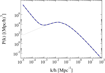
Figure 6: Cold dark matter power spectrum using the old gauge invariant implentation (dashed line) and the new strategy in gauge invariant variables (thin solid line). The density contrast shown is the gauge invariant combination $D_{g}^{cdm}\equiv\delta^{longit.}-3\phi$. The mean deviation between the curves is $\approx 0.02\%$. To guide the eye, we also depict the synchronous gauge power spectrum [thin gray dotted line]. The difference at large scales is due to gauge ambiguities. Again, we used $h=0.7$.

For the LSS evolution, neglecting the shear is a good approximation because Einstein’s Equation gives

$$\frac{12}{5}a^{2}\left[\bar{p}_{\gamma}\mathcal{M}_{2}+\bar{p}_{\nu}\mathcal{N}_{2}\right]=\textrm{M}_{\textrm{P}}^{2}k^{2}(\phi-\psi),$$ (31)

where $\mathcal{N}_{2}$ is the neutrino quadrupole. As $\bar{p}_{\gamma,\nu}\propto a^{-4}$, the difference of the metric potentials vanishes for small scale modes, i.e. at least

$$(\phi-\psi)\propto(ka)^{-2},$$ (32)

where we have neglected the decay of the quadrupoles $\mathcal{M}_{2}$ and $\mathcal{N}_{2}$ which give an additional suppression (see also Figure 6).

As the effect of $\delta_{\gamma}$ and $\mathcal{M}_{2}$ and $E_{2}$ at late times for small scale modes can be neglected (or very well approximated in the case of $\delta_{\gamma}$), we see that there is really no need to propagate relativistic species at later times. The key to our final speed up is therefore to avoid integrating these oscillations after they have become irrelevant. We do this by multiplying the RHS of equations (3 - 8) as well as the corresponding multipole evolution equations for relativistic neutrinos by a damping factor $\Gamma$. Defining $x\equiv k\tau$, we employ $\Gamma=\{1-\tanh([x-x_{c}]/w)\}/2$ with the cross over $x_{c}=\max(1000,k\tau_{dilute})$, where $a(\tau_{dilute})=5a_{equ}$ and $a_{equ}$ is the scale factor at matter-radiation equality. This later criterion ensures that the contribution of relativistic species to the perturbed energy densities is negligible: from equality on, $\delta_{c}\propto a$, whereas $\delta_{\gamma}$ decays and $\rho_{c}/\rho_{rel}\propto a^{-1}$ so at least

$$\delta_{c}\rho_{c}:\delta_{\gamma}\rho_{\gamma}\propto a^{-2},$$ (33)

and similar arguments hold for neutrinos. Hence, from $\tau_{dilute}$ on, one can safely ignore this contribution. The former criterion $x_{c}<1000$ ensures that oscillations have damped away sufficiently. The cross-over width $w$ is rather uncritical. We used $w=50$ to make the transition smooth. Typically, $\tau_{dilute}\approx 400\,\textrm{Mpc}$ and one therefore has to follow only a fraction of $\tau_{dilute}/\tau_{0}$ oscillations as compared to the standard strategy. This corresponds to a gain in efficiency by a factor $\tau_{0}/\tau_{dilute}\approx 30$.

To compute the sources $S_{T}$ and $S_{E}$, we use the expressions

$$\delta_{\gamma} = \Gamma\delta_{\gamma}^{numeric.}-4(1-\Gamma)\left[\psi+\frac{v_{b}}{k\tau_{c}}\right]$$ (34)

$$\mathcal{C} = \Gamma\mathcal{C}^{numeric.},$$ (35)

$$\dot{\mathcal{C}} = \Gamma\dot{\mathcal{C}}^{numeric.},$$ (36)

$$\ddot{\mathcal{C}} = \Gamma\ddot{\mathcal{C}}^{numeric.},$$ (37)

which interpolate between the numerical value before $\Gamma$-damping and the analytic approximations, Equation (27) and $\mathcal{C}\equiv 0$. Setting $\mathcal{C}\equiv 0$ is an approximation to the small value of the quadrupoles averaged over several oscillations.

For general dark energy models with rest frame speed of sound $c_{s}^{2}>0$ of the dark energy fluid, the dark energy perturbations well inside the horizon oscillate with high frequency. In this case, one needs to suppress the damped oscillations of the dark energy fluid perturbations much like those of photons to achieve faster integration.

IV Conclusions

We have improved the integration strategy of modern cosmological Boltzmann codes. As a first step, we made a conceptual distinction between tight coupling of the velocities $v_{\gamma}$ and $v_{b}$ and the validity of analytic estimates for the intensity and polarization quadrupole. Doing so allowed us to switch to the full numerical evolution later. The inclusion of shear at early times lead to an increase in precision. In the second part of our work, we investigated the behavior of photons after decoupling. We found analytic approximations for both $\delta_{\gamma}$ and $v_{\gamma}$ as well as a bound on the shear $\sigma_{\gamma}$. The contributions of photons and neutrinos towards CMB anisotropies can be well approximated by using these analytic estimates of $\delta_{\gamma}$ and $\sigma_{\gamma}$ for small scale modes deep inside the horizon. In fact, for an optical depth $\tau_{opt}\lessapprox 0.2$, late time effects of photons on the CMB anisotropy sources $S_{T}$ and $S_{E}$ may be neglected altogether on small scales. We introduced a smooth damping of high frequency oscillations of photon and neutrino multipoles. The damping effectively freezes their evolution well inside the horizon. All in all, our strategy leads to a gain in efficiency of up to factor $\sim 30$ and comes close to optimal accuracy for both the CMB and LSS.

Acknowledgments I would like to thank Max Tegmark for drawing my attention to this subject and Xue-Lei Chen and Constantinos Skordis for discussions about tight coupling. This work was supported by NSF grant PHY-0099543 at Dartmouth.

References

(1)
U. Seljak and M. Zaldarriaga,
Astrophys. J. 469 (1996) 437
[arXiv:astro-ph/9603033].
(2)
www.cmbfast.org
(3)
A. Lewis, A. Challinor and A. Lasenby,
Astrophys. J. 538 (2000) 473
[arXiv:astro-ph/9911177].
(4)
A. Lewis and S. Bridle,
Phys. Rev. D 66 (2002) 103511
[arXiv:astro-ph/0205436].
(5)
camb.info
(6)
M. Doran,
arXiv:astro-ph/0302138.
(7)
M. Doran and C. M. Mueller,
arXiv:astro-ph/0311311.
(8)
www.cmbeasy.org
(9)
D. N. Spergel et al. [WMAP Collaboration],
Astrophys. J. Suppl. 148, 175 (2003)
(10)
M. Tegmark et al. [SDSS Collaboration],
Phys. Rev. D 69 (2004) 103501
(11)
C. Skordis, Talk given at 1st Oxford-Princeton Workshop on Astrophysics and Cosmology,
Princeton (2003)
(12)
C. P. Ma and E. Bertschinger,
Astrophys. J. 455 (1995) 7
[arXiv:astro-ph/9506072].
(13)
P. J. Peebles and J. T. Yu,
Astrophys. J. 162 (1970) 815.