Metric Tests for Curvature from Weak Lensing and Baryon Acoustic Oscillations

Abstract

We describe a practical measurement of the curvature of the Universe which, unlike current constraints, relies purely on the properties of the Robertson-Walker metric rather than any assumed model for the dynamics and content of the Universe. The observable quantity is the cross-correlation between foreground mass and gravitational shear of background galaxies, which depends upon the angular diameter distances $d_{A}(z_{\ell})$, $d_{A}(z_{s})$, and $d_{A}(z_{s},z_{\ell})$ on the degenerate triangle formed by observer, source, and lens. In a flat Universe, $d_{A}(z_{\ell},z_{s})=d_{A}(z_{s})-d_{A}(z_{\ell})$, but in curved Universes an additional term $\propto\Omega_{k}$ appears and alters the lensing observables even if $d_{A}(z)$ is fixed. We describe a method whereby weak lensing data may be used to solve simultaneously for $d_{A}$ and the curvature. This method is completely insensitive to the equation of state of the contents of the Universe, or amendments to General Relativity that alter the gravitational deflection of light or the growth of structure. The curvature estimate is also independent of biases in the photometric redshift scale. This measurement is shown to be subject to a degeneracy among $d_{A}$, $\Omega_{k}$ and the galaxy bias factors that may be broken by using the same imaging data to measure the angular scale of baryon acoustic oscillations. Simplified estimates of the accuracy attainable by this method indicate that ambitious weak-lensing $+$ baryon-oscillation surveys would measure $\Omega_{k}$ to an accuracy $\approx 0.04f_{\rm sky}^{-1/2}(\sigma_{\ln z}/0.04)^{1/2}$, where $\sigma_{\ln z}$ is the photometric redshift error. The Fisher-matrix formalism developed here is also useful for predicting bounds on curvature and other characteristics of parametric dark-energy models. We forecast some representative error levels and compare to other analyses of the weak lensing cross-correlation method. We find both curvature and parametric constraints to be surprisingly insensitive to the systematic shear calibration errors.

1 Metric Measurements of Curvature

The most robust prediction of inflation theories is that the radius of curvature of the present Universe should be very large, i.e.  $\Omega_{k}=0$ to high accuracy. The WMAP$+$supernovae$+H_{0}$ best fit of $\Omega_{k}=-0.02\pm 0.02$ (Spergel et al., 2003) is therefore taken as a vindication of inflation, and a great majority of current work, such as investigations of the properties of dark energy, take $\Omega_{k}=0$ as a priori truth. It is important to realize, however, that WMAP does not measure curvature in any direct geometric way. Constraints on curvature derive primarily from a measurement of the angular diameter distance to recombination, $D_{A}(z_{\rm rec})$, which depends upon curvature but also upon $\Omega_{m}$ and models for dark energy or other constituents of the Universe. Hence the curvature results are dependent upon the $\Lambda$CDM (or other) model for dark energy assumed in the analysis. Our ignorance of the dark energy phenomenon limits our ability to test for flatness or to look for small finite $\Omega_{k}$ that may be predicted in variants of inflation (Uzan, Kirchner, & Ellis, 2003) or in Universes with non-trivial topology (Luminet et al., 2003).

Our ignorance of the true curvature will, conversely, foil attempts to characterize dark energy properties with Type Ia supernovae (or other standard candles), which measure $D_{L}(z)$ at lower redshifts. If the Tolman surface-brightness relation holds, then we have $D_{A}=D_{L}(1+z)^{-2}$. The proper-angular-diameter distance in a Universe with Robertson-Walker metric is

$$D_{A}(z) = (1+z)^{-1}S_{k}\left[r(z)\right],$$ (1)

$$S_{k}(r) \equiv \left\{\begin{array}[]{cl}R_{0}\sin(r/R_{0})&k=+1\\ r&k=0\\ R_{0}\sinh(r/R_{0})&k=-1\end{array}\right.$$ (5)

$$r(z) = c\int_{0}^{z}dzH^{-1}(z).$$ (6)

Here $r$ is the comoving radial distance, $R_{0}$ is the radius of curvature of the Universe, and $H(z)=\dot{a}/a$. These equations follow purely from the RW metric. If standard-candle and CMB observations were to give us perfect knowledge of $D_{A}(z)$, then for any $R_{0}$ and $k$ there is a solution

$${c\over H(z)}={d\over dz}S_{k}^{-1}\left[(1+z)D_{A}(z)\right].$$ (7)

that will exactly reproduce the data. If the Friedmann equations hold, then

$$H(z) = H_{0}\left[\Omega_{m}(1+z)^{3}+\Omega_{k}(1+z)^{2}+(1-\Omega_{m}-\Omega_{k})f_{X}(z)\right]^{1/2},$$ (8)

$$\Omega_{k} \equiv {-kc^{2}\over H_{0}^{2}R_{0}^{2}}.$$ (9)

Here $f_{X}(z)$ describes the evolution of $\rho_{X}$, an additional dark-energy component. Hence even with perfect knowledge of $D_{A}(z)$, there is always some dark energy behavior $f_{X}$ which reproduces that data for any choice of curvature. The degeneracy between curvature and dynamics is well known, e.g.  Weinberg (1970) demonstrates that even complete knowledge of $D_{A}(z)$ cannot constrain the curvature in the absence of a dynamical model for the expansion. Constraints on curvature from $D_{A}$ data arise solely because of our preferences for forms of $f_{X}$ that arise from certain equations of state. Allowing alterations to the Friedmann equations adds additional degeneracy.

We can break the degeneracy between curvature and $f_{X}$ without making dynamical assumptions if we apply the metric to some line segment that does not originate at $z=0$, essentially forming a cosmological-scale triangle. For example if a gravitational lens at $z_{\ell}$ bends a light ray by angle $\alpha$, then the apparent deflection of a source at $z_{s}$ observed from $z=0$ obeys

$$\delta\theta=\alpha{D_{A}(z_{\ell},z_{s})\over D_{A}(z_{s})},$$ (10)

where $D_{A}(z_{\ell},z_{s})$ is the proper angular-diameter distance at $z_{s}$ as viewed from $z_{\ell}$. We introduce a dimensionless comoving angular diameter distance

$$d(z_{1},z_{2}) \equiv {H_{0}\over c}(1+z_{2})D_{A}(z_{1},z_{2})$$ (11)

$$= S(\chi_{2}-\chi_{1}),$$ (12)

$$\chi \equiv {H_{0}\over c}r,$$ (13)

$$d(z) \equiv d(0,z)$$ (14)

$$S(\chi) = \left\{\begin{array}[]{cl}\chi_{0}\sin(\chi/\chi_{0})&k=+1\\ \chi&k=0\\ \chi_{0}\sinh(\chi/\chi_{0})&k=-1\end{array}\right.$$ (18)

Now $\chi_{0}$ is the radius of curvature in Hubble lengths. Using the difference rule for $S(\chi)$ we obtain

$$d(z_{\ell},z_{s}) = S(\chi_{s}-\chi_{\ell})$$ (19)

$$= S(\chi_{s})C(\chi_{\ell})-S(\chi_{\ell})C(\chi_{s})$$ (20)

$$C(\chi) \equiv \left\{\begin{array}[]{cl}\cos(\chi/\chi_{0})&k=+1\\ 1&k=0\\ \cosh(\chi/\chi_{0})&k=-1\end{array}\right.$$ (24)

$$\Rightarrow\quad d(z_{\ell},z_{s}) = S(\chi_{s})\left[1+{\Omega_{k}\over 2}S^{2}(\chi_{\ell})\right]-S(\chi_{\ell})\left[1+{\Omega_{k}\over 2}S^{2}(\chi_{s})\right]+O(\Omega_{k}^{2})$$ (25)

$$= (d_{s}-d_{\ell})(1-\Omega_{k}d_{\ell}d_{s}/2)+O(\Omega_{k}^{2}).$$ (26)

So while the $d(z)$ function itself has a curvature-dark energy degeneracy, the lensing strength depends purely on $\Omega_{k}$ once $d(z)$ is known, e.g.  from supernova measurements. This $\Omega_{k}$ dependence is well known, e.g.  Equation (13.70) in Peebles (1993). Figure 1 illustrates how the curvature of the Universe is indeterminate when distances from $z=0$ are the only observables, whereas a measure of $d_{\ell s}$ determines curvature. Linder (1988) remarks that the presence of this differential distance in gravitational lensing equations could provide useful cosmological tests, but to our knowledge no practical implementation of this—or any other—metric curvature test has been proposed.

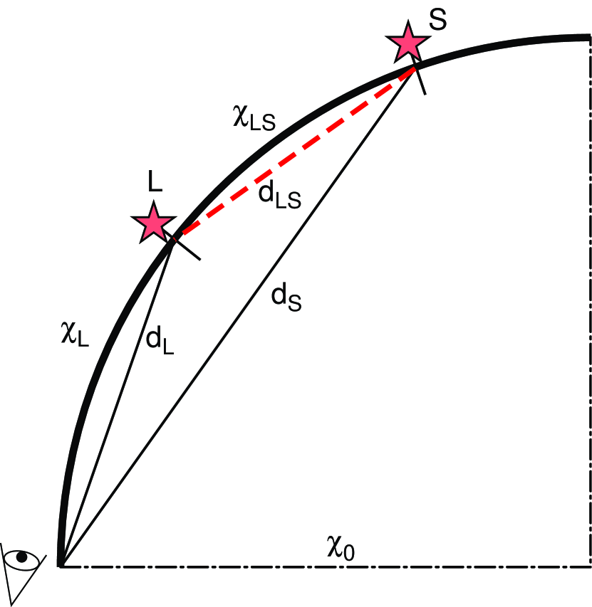
Figure 1: Illustration of curvature determination: consider an observer on a section of the closed Universe, represented by the bold line. The conformal distances $\chi_{L}$ and $\chi_{S}$ to two sources are not directly observable; only the angular-diameter distances are, $d_{L}$ and $d_{S}$ represented here by the chord lengths. The radius of curvature $\chi_{0}$ is indeterminate, but a measure of the distance $d_{LS}$ (dashed line) allows determination of the curvature.

We propose that $\Omega_{k}$ be determined by measuring the gravitational lensing shear $\gamma$ of background galaxies—i.e.  the gradient of $\delta\theta$ in Equation (10)—and measuring the amplitude of the contribution from the $O(\Omega_{k})$ term in Equation (26). A foolishly optimistic estimate of the accuracy available on $\Omega_{k}$ can be obtained by assuming that the deflection angles $\alpha$ are known a priori at all redshifts and positions on the sky, and that the angular diameter distance $d(z)$ has been measured as well. Since $d_{\ell}$ and $d_{s}$ are in the range 0.5–1.5 at relevant distances for weak lensing in the $\Lambda$CDM fiducial model, the lensing shear scales as $\approx(1-\Omega_{k}/2)$, so we would find that $\delta\Omega_{k}\approx 2\delta\gamma/\gamma$. The typical shear amplitude $\gamma$ over a line of sight is $\approx 0.02$ at cosmological distances. The uncertainty in shear is $\approx 0.3/\sqrt{N}_{g}$, where $N_{g}$ is the number of galaxies with well-measured shapes. A space-based survey can measure 100 galaxies per square arcminute, which leads to $\delta\Omega_{k}\sim 0.0002/\sqrt{f}_{\rm sky}$, far better than the current model-dependent constraints. This estimate is unrealistic, however, because neither the distance functions nor the deflections will be known. Below we will investigate a simultaneous solution for the angular-diameter distances, deflection strengths, and $\Omega_{k}$ from cross-correlation of lensing shear with foreground galaxy distributions, and estimate the resultant degradation in the curvature constraint.

If we execute the WL curvature measurement by dividing our galaxy sample into redshift bins, then we note that we do not actually need to know the redshift of each bin; it is only the distance $d$ of each bin that enters into the calculation of the shear. Hence biases in photometric redshifts do not affect the curvature measurement. It is essential, however, to insure that the galaxies in a bin are at a common distance.

In the remainder of this section we examine metric tests for curvature which might be possible with other cosmological observables besides weak lensing. In §2 we develop the methodology for using weak lensing cross-correlations to solve simultaneously for the curvature, distance relationships, and deflector properties. The implementation is significantly more involved and subtle than the simple idea that curvature is manifested in $d_{\ell s}$. §3 applies the formalism to forecast curvature constraints from feasible surveys, and extends the formalism to include treatment of the likely dominant systematic error. §4 investigates the constraints on parametric models of dark energy ($w_{0}$,$w_{a}$) that can be derived with the curvature left free to vary, and compares the present results to some previous work on weak lensing cross-correlations. §5 summarizes and concludes.

1.1 Metric Curvature from Other Cosmological Measurements

Similarly metric determinations of $\Omega_{k}$ are in principle derivable from other cosmological measurements. The most promising is the detection of the recombination acoustic horizon scale, which is known in comoving physical units from the CMB, in the power spectrum of galaxies, recently demonstrated by Eisenstein et al. (2005). The transverse baryon acoustic oscillation (BAO) test measures the angular scale subtended by this standard ruler, and hence measures $(1+z)D_{A}(z)\propto h^{-1}d(z)$. The transverse BAO method does not by itself break the curvature-dark energy degeneracy, but may serve as a source of high-reliability constraints on $d(z)$ to combine with weak lensing information. Again for a given galaxy subsample, the redshift itself is unimportant, just the observable $d$.

With sufficient redshift resolution, the acoustic scale may be identified along the line of sight, yielding knowledge of

$${dr\over dz}={c\over H_{0}}d^{\prime}(z)(1-\Omega_{k}d^{2}/2)+O(\Omega_{k}^{2}).$$ (27)

Hence the comparison of line-of-sight to transverse BAO scales can yield $\Omega_{k}$ directly, but requires one to either integrate the line-of-sight $H(z)$ data or differentiate the transverse $d(z)$ data. Doing either operation in the presence of noise adds substantial difficulties to making a high-accuracy comparison, unless one assumes a parametric form for $d(z)$.

Counts of galaxy clusters are sensitive to $dV/d\Omega\,dz\propto h^{-3}d^{2}d^{\prime}(z)(1-\Omega_{k}d^{2}/2)$. Volume-element data alone can not measure $\Omega_{k}$, but could potentially do so in combination with high-precision measures of $d(z)$ and its derivative. Cluster counts are also, however, dependent upon the growth of structure, so do not offer the model-independent cosmographic information of weak lensing or baryon oscillations.

Stellar evolution has been proposed as a standard chronometer (Jimenez et al., 2003), which could determine $H(z)$ and hence the curvature if combined with measures of $d$. To contribute to the metric measurement of curvature, accuracies of a few percent on $H(z)$ are required, and further investigation into the complexities of stellar and galactic evolution are needed in order to determine whether robust constraints at this accuracy are possible.

Strong lensing may also be used to discern the behavior of $d(z_{\ell},z_{s})/d(z_{s})$, if one is presented with a lensing system with multiply-imaged sources at a variety of (known) background redshifts. Such use of multiple arcs around clusters has been investigated in the context of constraining dark energy (Link & Pierce, 1998; Gautret, Fort, & Mellier, 2000; Golse, Kneib, & Soucail, 2002; Sereno, 2002; Soucail et al., 2004), and would be equally applicable to determination of curvature, but also equally susceptible to the small uncertainties in the mass profiles of clusters.

2 Cosmographic Methodology

The metric curvature determination is clearly an extension of the cross-correlation cosmography (CCC) technique proposed by Jain & Taylor (2003): one identifies rich foreground clusters and measures the dependence of the induced background shear upon $z_{s}$ of the source galaxies. The mass of the cluster(s) may be unknown, but the ratio of any two background shears is a purely cosmographic function. Song & Knox (2004) combine this approach with other dark energy probes. Bernstein & Jain (2004)[BJ04] generalize the method to a cross-correlation between foreground estimated-mass distributions and background shear patterns. In this case the cluster-mass uncertainty is replaced by an unknown bias factor for each foreground mass shell, over which we marginalize. Zhang, Hui, & Stebbins (2003)[ZHS] give a more elegant analysis in which the galaxy-shear cross-correlations are considered simultaneously with the shear-shear correlations in a single Fisher matrix. Hu & Jain (2004) also include the galaxy-galaxy correlations in the same Fisher matrix, and make use of a parametric model of bias based on the halo model of galaxy distributions. All of these analyses differ substantially in their analytic approaches, underlying assumptions, and estimated constraints. A full comparison is beyond the scope of this paper, but we will make some brief comments below. Here we attempt to recast the problem in a manner suited to the metric curvature constraint, but also amenable to studying the parametric dark-energy constraints investigated by these authors.

The shear induced in direction $\theta$ on sources at $z_{s}$ by mass in the foreground can be decomposed into $E$- and $B$-mode components. In the weak-lensing limit, the former is straightforwardly related to the lensing convergence $\kappa$ and the latter should vanish. Hence we will consider the shape information to come in the form of the convergence field $\kappa$, which depends upon direction and source redshift as

$$\kappa(\mbox{\boldmath$\theta$},z_{s})={3\Omega_{m}\over 2}\int_{0}^{z_{s}}dz_{\ell}{d_{\ell}(1+z_{\ell})H_{0}\over H(z_{\ell})}m({\mbox{\boldmath$\theta$}},z_{\ell}){d_{s}-d_{\ell}\over d_{s}}(1-\Omega_{k}d_{s}d_{\ell}/2),$$ (28)

where $m$ is the overdensity $\delta\rho/\bar{\rho}$ of the total mass.

We also idealize the sky as consisting of $K$ discrete pencil-beams of solid angle $\delta\Omega$, with the true mass density $m(\mbox{\boldmath$\theta$}_{i})$ being statistically independent of the density in any other beam. We can choose $\delta\Omega$ to correspond to a correlation length of the true continuum shear field. We will assume $\delta\Omega=0.25\,{\rm arcmin}^{2}$; the results depend only weakly on this choice. We could equivalently decompose the shear and mass distributions into spherical harmonics, in which case our choice of $\delta\Omega$ becomes equivalent to a maximum multipole $\ell\approx 2\times 10^{4}$.

The weak lensing equation (28) can be written

$$\kappa(s,\mbox{\boldmath$\theta$}_{i}) = \int d\ell\,G(s,\ell)m(\ell,\mbox{\boldmath$\theta$}_{i})k(\ell),$$ (29)

$$k(\ell) \equiv {3\Omega_{m}\over 2}\ell(1+z_{\ell})(1-\Omega_{k}\ell^{2}/2)$$ (30)

$$G(s,\ell) = \left(1-{\ell\over s}\right)(1-\Omega_{k}s\ell/2)\Theta(s-\ell),$$ (31)

where $\Theta$ is the step function, and we have reparameterized the source- and lens-plane distances by $s=d(z_{s})$, $\ell=d(z_{\ell})$. This equation assumes the validity of General Relativity in two respects: first, that light follows the geodesic equation for the metric, and second, that we have the usual Poisson equation. The second assumption can be dropped in our quest for a purely metric test of curvature. In our formalism a change of the Poisson equation would be accommodated by generalizing $k_{\ell}m(\ell,\mbox{\boldmath$\theta$})$ to mean the convergence caused by the mass at distance $\ell$, even if this means that $m$ is no longer the unaltered mass distribution.

We discretize the analysis by considering the galaxies to be located on a series of $J$ shells, in order to facilitate the construction of Fisher matrices below. The finite thickness of the shells complicates the analysis (ZHS) and in fact it is possible to draw erroneous conclusions from a discrete analysis, as discussed by Stebbins (2005). Below we will attempt to return the discrete formulation to the continuum limit and discuss these issues.

The measured shear at each source plane becomes, with a noise term now added,

$$\kappa_{s}(\mbox{\boldmath$\theta$}_{i}) = \sum_{\ell}G_{s\ell}m_{\ell}(\mbox{\boldmath$\theta$}_{i})k_{\ell}+(\delta\kappa)_{s}(\mbox{\boldmath$\theta$}_{i}),$$ (32)

$$G_{s\ell} = \left\{\begin{array}[]{cl}{d_{s}-d_{\ell}\over d_{s}}(1-\Omega_{k}d_{s}d_{\ell}/2)&\ell<s\\ 0&\ell\geq s\end{array}\right.$$ (35)

$${\rm Var}(\delta\kappa_{s}) = {\sigma_{\gamma}\over\sqrt{n_{s}\,\delta\Omega}},$$ (36)

$$k_{\ell} \equiv {3\Omega_{m}\over 2}d_{\ell}(1+z_{\ell})\Delta\chi={3\Omega_{m}\over 2}d_{\ell}(1+z_{\ell})(1-\Omega_{k}d_{\ell}^{2}/2)\Delta d_{\ell}.$$ (37)

Now $m_{\ell}(\mbox{\boldmath$\theta$})$ is the mass overdensity averaged through the shell of width $\Delta\chi$; $k_{\ell}$ is a factor that converts this overdensity into the convergence measured on a lens plane at infinity. The shear measurement noise is determined by the areal density $n_{s}$ of shape-measurable galaxies on shell $s$, and $\sigma_{\gamma}\approx 0.3$ (Bernstein, 2005).

The true mass fluctuation $m_{\ell}(\mbox{\boldmath$\theta$})$ is not directly observable. But we assume that we deduce from the galaxy distribution some estimate of the mass overdensity $g_{\ell}(\mbox{\boldmath$\theta$})$ that is correlated with the true distribution. This proxy field need not be the galaxy density itself, but rather the result of any algorithm applied to the observed galaxy field, e.g.  involving the assignment of halos to galaxies, groups, and clusters. The correlation coefficient of the true and proxy mass fields is

$${\langle m_{i}g_{j}\rangle\over\sqrt{\langle m_{i}^{2}\rangle\langle g_{j}^{2}\rangle}}=\delta_{ij}r_{i},$$ (38)

where the angle brackets denote averaging over direction $\theta$. The $r_{i}$ are not known but are assumed positive. We assume that the shells are thick enough to be uncorrelated. We also define for each shell an unknown bias via

$$\langle m_{i}g_{i}\rangle=B_{i}\langle g_{i}^{2}\rangle.$$ (39)

Note that this is the bias of the true mass with respect to the estimated mass. The more conventional bias $b$ of the estimated (galaxy) mass to the true mass is, for Gaussian-distributed $g$ and $m$, related to this via

$$B_{i}={r_{i}^{2}\over b_{i}}.$$ (40)

The shear noise $\delta\kappa$ is assumed to have correlations with neither the true nor the proxy mass distribution.

With these definitions we could extract curvature information from our observed shear data as follows: we cross-correlate each convergence field $\kappa_{s}$ with each foreground proxy field $g_{\ell}$ to give an observable quantity $X_{s\ell}$. From Equation (32) the expectation values are

$$\langle X_{s\ell}\rangle=\sum_{\ell^{\prime}}G_{s\ell^{\prime}}k_{\ell^{\prime}}\langle g_{\ell}m_{\ell^{\prime}}\rangle=G_{s\ell}B_{\ell}k_{\ell}\langle g_{\ell}^{2}\rangle.$$ (41)

There are $J(J-1)/2$ non-zero observable cross-correlations, which are statistically independent for any significant sky coverage. These $X_{s\ell}$ are determined by the $J$ factors $(B_{\ell}k_{\ell}\langle g_{\ell}^{2}\rangle)$, plus the matrix ${\bf G}$ that is defined by $J$ distances $d_{i}$ and the single $\Omega_{k}$. Hence there are $2J+1$ free parameters, so we might expect an unambiguous fit to the data for $J\geq 5$. After marginalization over the nuisance parameters $B_{i}$ and $d_{i}$ (which carry much information about dark energy and galaxy formation!) one obtains constraints on $\Omega_{k}$.

Unfortunately the simultaneous solution for $\Omega_{k}$, ${\bf B}$, and ${\bf d}$ from the system of equations (41) has three degeneracies in the neighborhood of $\Omega_{k}=0$. The transformations

$$d_{i}\rightarrow d_{i}(1+\alpha_{0})$$ (42)

$$d_{i}\rightarrow d_{i}/(1-\alpha_{1}d_{i}),\quad(B_{i}k_{i})\rightarrow(B_{i}k_{i})(1-\alpha_{1}d_{i})$$ (43)

$$d_{i}\rightarrow d_{i}/(1-\alpha_{2}d_{i}^{2}),\quad(B_{i}k_{i})\rightarrow(B_{i}k_{i})(1-\alpha_{2}d_{i}^{2}),\quad\Omega_{k}\rightarrow\Omega_{k}+2\alpha_{2}$$ (44)

each leave the observable shear unchanged to first order in $\Omega_{k}$ and the free parameters $\alpha_{i}$. The first degeneracy is a simple scaling of the $d_{i}$, which is unsurprising as the lensing observables depend only upon distance ratios. The second degeneracy is similarly benign as it leaves the solution for $\Omega_{k}$ unchanged. But the third degeneracy leaves $\Omega_{k}$ indeterminate. The degeneracy can be broken if we assume some functional form for $d(z)$, but our goal is a model-independent constraint. The same imaging survey that is used to generate the shear measurement and the foreground galaxy maps can be used to measure the transverse baryon acoustic horizon scale, if the photometric redshift accuracy $\sigma_{\ln z}$ is sufficiently good. This will produce a statistically independent measure of $d_{i}$ at each shell, which we may use to break the curvature degeneracy that remains in the lensing cross-correlations.

There is a more subtle problem with a solution for cosmology via Equation (41). As noted by Stebbins (2005), the solution offers no discriminatory power on cosmology if we allow the $B_{i}$ to be completely free, because the matrix $G_{s\ell}$ must be invertible as we approach the continuum limit. Looking explicitly at the continuum limit in Equation (29), Stebbins shows that there must always be some function $G^{-1}(\ell,s)$ such that

$$m(\ell)k(\ell)=\int ds\,G^{-1}(\ell,s)\kappa(s).$$ (45)

In fact we can construct this function explicitly to first order in $\Omega_{k}$:

$$G^{-1}(\ell,s) = \left(1+{\Omega_{k}\over 2}\ell^{2}\right)s\delta^{\prime\prime}(s-\ell)+\Omega_{k}\ell s\delta^{\prime}(s-\ell)$$ (46)

$$\Rightarrow\qquad m(\ell)k(\ell) = \left(1+{\Omega_{k}\over 2}\ell^{2}\right)\left.{d^{2}(s\kappa)\over ds^{2}}\right|_{\ell}+\Omega_{k}\ell s\left.{d(s\kappa)\over ds}\right|_{\ell}.$$ (47)

Here $\delta$ is the Dirac function. Surprisingly this inversion of the lensing cross-correlation is local. Given this solution, we simply set $B(\ell)=m(\ell)/g(\ell)$ and get an exact solution on this line of sight, regardless of our choice of $\Omega_{k}$ and $d(z)$ functions. There is hence no possibility of inference of cosmological parameters along this line of sight as we reach the continuum limit. Similarly a solution of the cross-correlation Equation (41) is possible for any choice of cosmology, once we reach a large number of lens and source planes, as $G$ is always invertible to give a valid ${\bf B}$.

An exit from this conundrum is the realization that giving complete freedom to the bias function $B(\ell)$ is tantamount to discarding our initial presumption that the proxy field is correlated with the true mass distribution. Imagine slicing the Universe so finely as to assign each proton its own bias value with respect to the dark matter. With this freedom we could clearly produce any macroscopic mass distribution we wish, including one that has no correlation at all with the galaxy-scale baryon distribution. We must therefore incorporate into the analysis some criteria for the coherence of the bias parameter in order to reflect our underlying assumption that mass has some correlation with the proxy field.

We note, for example, that the continuum-limit inversion formula Equation (46) will produce a divergent solution for $m(\ell)$ in the presence of any finite amount of shot noise on the lensing field $\kappa(s)$. The cross-correlation between estimated $m(\ell)$ and $g(\ell)$ can be estimated from the multiple lines of sight in the survey, and will be driven to zero in this continuum limit. If the likelihood function for our joint analysis of the $\kappa$ and $g$ fields requires them to be correlated Gaussian variables, then the rapidly varying components of the inversion solution for $m$ will be suppressed in a maximum-likelihood solution, and it becomes possible to discriminate cosmologies.

We do not claim yet to have a rigorous model-independent method to approach the continuum limit. Below we produce a likelihood function for the shear and proxy fields that incorporates their presumed correlation on scales of a shell thickness. Our practical approach will be to see how the uncertainties in our cosmological parameters scale as the number of shells increases; in fact we see no significant changes in any of the results below as we decrease the shell size as far as $\Delta z\approx 0.02$. Another practical approach that we will take is to include a regularization condition on $B(\ell)$ to lower the probability of solutions that vary rapidly on short redshift (and hence time) scales, in accordance with our physical intuition; this too has no significant impact upon our forecasts.

A potentially more enlightening approach to the cross-correlation problem may be to parameterize the functions $d(z)$ and $B(z)$ by expansions in orthonormal function sets, such as Fourier modes or Legendre polynomials, rather than assume a stepwise variation and/or discrete galaxy distributions.

2.1 Likelihood Function

The accuracy of constraints on $\Omega_{k}$ can be estimated by the Fisher matrix methodology. We produce a Fisher matrix for a single line of sight, and then multiply by $K$ since we have assumed all lines of sight to be independent. On each line of sight there are three $J$-dimensional vectors: the measured convergence $\kappa$; the true mass distribution ${\bf m}$; and the proxy mass estimate ${\bf g}$. We need a likelihood function $L(\mbox{\boldmath$\kappa$},{\bf m},{\bf g})$, which we then must marginalize over the unobservable ${\bf m}$. This probability can be expressed as

$$L(\mbox{\boldmath$\kappa$},{\bf m},{\bf g})=L(\mbox{\boldmath$\kappa$}|{\bf m})L({\bf m},{\bf g}).$$ (48)

Since the shear measurements arise from the sum of many individual galaxy shape measurements, the shear measurement noise is well expressed as a Gaussian distribution, so the first term is

$$L(\mbox{\boldmath$\kappa$}|{\bf m})=(2\pi)^{-J/2}|{\bf N}|^{-1/2}\exp\left\{-{1\over 2}\left[(\mbox{\boldmath$\kappa$}-{\bf G}{\bf km})^{T}{\bf N}^{-1}(\mbox{\boldmath$\kappa$}-{\bf G}{\bf km})\right]\right\}.$$ (49)

where ${\bf N}$ is the convergence noise matrix ${\rm diag}(\langle\delta\kappa^{2}_{s}\rangle)$, and ${\bf k}={\rm diag}(k_{\ell})$.

For analytical convenience we take the joint probability $L({\bf m},{\bf g})$ of the true and estimated masses to be a bivariate Gaussian at each slice. This is undoubtedly a poor approximation, e.g.  most of the lensing cross-correlation power is on angular scales where the mass distribution is highly non-linear and non-Gaussian. We defer a more realistic treatment to later work. Given our definition of the bias $B_{i}$ and correlation coefficient $r_{i}$, the probability can be written

$$L({\bf m},{\bf g}) = (2\pi)^{-J}|{\bf C_{u}}|^{-1/2}|{\bf C_{g}}|^{-1/2}\exp\left\{-{1\over 2}\left[({\bf m}-{\bf B}{\bf g})^{T}{\bf C_{u}}^{-1}({\bf m}-{\bf B}{\bf g})+{\bf g}^{T}{\bf C_{g}}^{-1}{\bf g}\right]\right\}$$ (50)

$${\bf C_{g}} \equiv {\rm diag}(\langle g_{i}^{2}\rangle)$$ (51)

$${\bf B} \equiv {\rm diag}(B_{i})$$ (52)

$${\bf C_{u}} \equiv {\rm diag}\left({B_{i}^{2}(1-r_{i}^{2})\over r_{i}^{2}}\langle g_{i}^{2}\rangle\right)={\rm diag}\left[\langle m_{i}^{2}\rangle(1-r_{i}^{2})\right].$$ (53)

${\bf C_{g}}$ is the correlation matrix for the mass estimator, and ${\bf C_{u}}$ is the correlation matrix for the part of the mass fluctuations that are uncorrelated with the estimator ${\bf g}$. We assume the shells are thick enough for both matrices to be diagonal.

Multiplying Equations (49) and (50), then integrating over ${\bf m}$ gives the Gaussian distribution

$$L(\mbox{\boldmath$\kappa$},{\bf g}) = (2\pi)^{-J}|{\bf KC_{g}}|^{-1/2}\exp\left\{-{1\over 2}\left[{\bf g}^{T}{\bf C_{g}}^{-1}{\bf g}+(\mbox{\boldmath$\kappa$}-{\bf GkBg})^{T}{\bf K}^{-1}(\mbox{\boldmath$\kappa$}-{\bf GkBg})\right]\right\},$$ (54)

$${\bf K} = {\bf N}+{\bf GkC_{u}k}^{T}{\bf G}^{T}.$$ (55)

${\bf K}$ is the covariance matrix for $\kappa$ if the mass estimators $g$ are held fixed, i.e.  only the components of the mass distribution that are uncorrelated with $g$ are considered stochastic.

From this multivariate Gaussian distribution we may derive a Fisher matrix using the formulae for zero-mean distribution given, e.g. , by Tegmark, Taylor, & Heavens (1997). We also multiply this by the number of independent lines of sight in the survey to get

$$F_{ij}={4\pi f_{\rm sky}\over\delta\Omega}{\rm Tr}\left[{\bf C_{g}}^{-1}{\bf C_{g}}_{,i}{\bf C_{g}}^{-1}{\bf C_{g}}_{,j}+{\bf K}^{-1}{\bf K}_{,i}{\bf K}^{-1}{\bf K}_{,j}+2{\bf K}^{-1}({\bf GkB})_{,i}{\bf C_{g}}({\bf GkB})^{T}_{,j}\right],$$ (56)

with the commas in the subscripts denoting differentiation. The Fisher information nicely separates into three parts: the first is the information that can be gleaned from the variances of the mass estimator $g$, i.e.  the galaxy power spectrum. The third term is Fisher information that would arise from adjusting parameters to minimize the $\chi^{2}$ in the fit of $\kappa$ to the estimated mass $g$ in Equation (32), were the values of $g$ taken as fixed and the matrix ${\bf K}$ taken as a known covariance for the $\kappa$ values. The third term is information gleaned from the actual covariance of the $\kappa$ residuals to this fit, and looks just like the Fisher matrix for pure shear power-spectrum tomography, except that the relevant mass power spectrum in this term is ${\bf C_{u}}$, the power that is uncorrelated with the galaxies, not the (larger) total power of $m$. Hence the inclusion of cross-correlation will lower the sample variance in lensing power-spectrum tomography.

In this paper we will presume that none of the (co-)variances of the true or estimated mass distributions are well predicted by theory. Hence we will marginalize over $C_{g},B$, and $C_{u}$ at each redshift. There will be no cosmological information gleaned from analysis of ${\bf C_{g}}$ since we consider its elements to be free parameters of the model, hence we can drop the first term of Equation (56).

Since we are marginalizing over all the mass variances, we can also absorb the overdensity-to-convergence conversion factor $k_{\ell}$ into the definition of $m_{\ell}$ and $g_{\ell}$, and remove it from Equations (55) and (56). We just must remember to express our fiducial values of $C_{u}$ and $C_{g}$ as convergence variances rather than as overdensity variances.

In a future paper we will consider cases where there are reliable theoretical models for the mass fluctuations. Hu & Jain (2004) consider the case where not only the mass power spectrum but also the bias and correlation of the galaxy sample are described by parametric models.

To recap, then, we will use the Fisher matrix

$$F_{ij} = {4\pi f_{\rm sky}\over\delta\Omega}{\rm Tr}\left[{\bf K}^{-1}{\bf K}_{,i}{\bf K}^{-1}{\bf K}_{,j}+2{\bf K}^{-1}({\bf GB})_{,i}{\bf C_{g}}({\bf GB})^{T}_{,j}\right],$$ (57)

$${\bf K} \equiv {\bf N}+{\bf GC_{u}}{\bf G}^{T}.$$ (58)

with the parameters being:

• $\Omega_{k}$, which affects only ${\bf G}$. The fiducial value is zero.

• The $d_{i}$, which also only affect ${\bf G}$. The fiducial values at each redshift are taken from the $\Lambda$CDM model with $\Omega_{m}=0.3$.

• The diagonal elements of ${\bf C_{u}}$, over which we will marginalize to allow for our ignorance of the cross-correlations $r_{\ell}$ between the proxy and true mass distributions. We take a fiducial $r_{\ell}=0.7$ but investigate the effect of different fiducial values.

• The diagonal elements $B_{i}$ of ${\bf B}$, the bias factors, over which we will marginalize. We take the fiducial $B_{i}=1$ without loss of generality.

• The diagonal elements of ${\bf C_{g}}$ are also free parameters, but striking the first term of (56) is equivalent to marginalizing over these parameters.

With these parameters, all of the derivatives required in Equation (57) are simple, sparse matrices.

2.2 Additional Information

The CCC Fisher matrix will be singular due to the degeneracies in the parameters noted above. To this we must add a Fisher matrix for the $d_{i}$ determined from the baryon acoustic oscillations; this matrix will be diagonal as the galaxy power spectrum measurements are independent from shell to shell if the shells are much thicker than the acoustic horizon scale.

For the baryon acoustic scale measurement, we use an abstraction of the full analysis provided by Seo & Eisenstein (2003). We presume that there is a fractional uncertainty $\sigma_{\ln(1+z)}$ in $1+z$ on each photometric redshift, which defines the depth of a “slab” of modes in $k$-space that are measurable. We also presume that the power spectrum determination for all modes within the slab will be limited by sample variance, which requires that the comoving volume density of galaxies with good photo-z’s must be $dN/dV\gtrsim 10^{-3}h^{3}\,{\rm Mpc}^{-3}=10^{7.5}(H_{0}/c)^{3}$ to make the shot noise negligible at the highest $k\approx 0.2h\,{\rm Mpc}^{-1}$ where baryon oscillations are usefully detected. When these conditions are met, the fractional error in the mean $d$ for a given shell will scale as $\sqrt{\sigma_{\ln(1+z)}/V}$. The prefactor depends upon the intensity of the wiggles in $P(k)$, which diminishes somewhat at lower redshift as nonlinear effects erase the acoustic features. We approximate this by assigning an uncertainty

$${\sigma_{d}\over d}=0.005\left({1+z\over 2+z}\right)(VH_{0}^{3}/c^{3})^{-1/2}\left({\sigma_{\ln(1+z)}\over 0.04}\right)^{1/2}$$ (59)

for those shells which, by Equation (61), have $dN/dV$ above the sample-variance-limited threshold noted above. If the galaxy density in the shell is below this level, we assume no constraint on $d$ from BAO. Our simplification fits the Seo & Eisenstein (2003) results well and comes within 30% of the forecasts by Glazebrook & Blake (2005).

We will also investigate the impact of a regularization constraint on the $B$ function. Writing the bias as a function of the lens-plane angular diameter distance $\ell$, we add to the likelihood a function

$$-\ln L={1\over R^{2}\ell_{\rm max}}\int_{0}^{\ell_{\rm max}}d\ell\,\left({dB\over d\ell}\right)^{2}.$$ (60)

The parameter $R$ specifies a scale of the RMS bias slope that will be suppressed. The discretized version of this likelihood is a quadratic form in the $B_{i}$ and easily incorporated into the Fisher matrix. We project the three degeneracies in Equations (42–44) out of the ${\bf B}$ vector before applying the regularization constraint, so that the regularization does not artificially break these degeneracies.

3 Curvature Forecasts

We calculate the Fisher matrix about our fiducial cosmology using the following estimates for the relevant quantities.

The $\kappa$ variances in ${\bf N}$ are taken from Equation (36) with the source galaxies distributed as

$${dn\over dz}\propto z^{2}\exp\left[-(z/1.41z_{0})^{1.5}\right],$$ (61)

with the median redshift $z_{0}$ and the integrated density $n$ chosen to crudely mimic the expectations of future surveys. Our default is to take $z_{0}=1.5$, $n=100\,{\rm arcmin}^{-2}$, the performance one might expect from a space-based survey like the proposed SNAP wide survey (Massey et al., 2004; Bernstein, 2005).

We set the variance $\langle m^{2}_{\ell}\rangle$ to the convergence variance $d\langle\kappa^{2}\rangle/dz$ integrated over each shell, using the nonlinear dark-matter power spectrum for a $\Lambda$CDM model, restricted to $k<2\pi/(50~{}{\rm kpc})$, as detailed in BJ04. Given a fiducial correlation coefficient $r$, we set $\langle g_{\ell}^{2}\rangle=r^{2}\langle m_{\ell}^{2}\rangle$. We will set all the fiducial $r_{\ell}=0.7$, although the marginalization allows them to have independent solutions.

We also truncate the source and lens distributions at $z_{\rm max}=3$ unless otherwise noted. The number of redshift bins will range from 30 to $\approx 200$ to search for effects of the artificial discretization of the problem.

3.1 Constraints on $\Omega_{k}$

The Fisher matrix for the fiducial cosmology yields, first, an estimate of the uncertainty on $\Omega_{k}$ of $\sigma_{k}=1.6\times 10^{-4}f_{\rm sky}^{-1/2}$ in the unrealistic case where all the biases, distances, and correlation coefficients are known a priori. This is in good agreement with our crude guess earlier.

When we marginalize over all parameters except $\Omega_{k}$, we find that if we project out the degeneracy in Equation (44), then the weak lensing CCC method is remarkably efficient at extracting $\Omega_{k}$, giving an uncertainty $\sigma_{k}\approx 2\times 10^{-4}f_{\rm sky}^{-1/2}$, nearly as good as before any marginalization. Of course this is akin to stating that the Titanic was watertight, aside from the big gash from the iceberg. Nonetheless this feature of the CCC method is illuminating: it tells us that the role of other distance measures, i.e.  supernovae and transverse BAO, will be purely to bound the size of the quadratic degeneracy in the CCC distances that couples to $\Omega_{k}$, because the CCC method reduces any other form of uncertainty in $d(z)$ and $\Omega_{k}$ to far below the level achievable from such experiments.

If, for example, we remove the three singular values from the WL-only Fisher matrix, and then estimate the uncertainties in $d(z)$, we find $\sigma_{d}\approx 1.4\times 10^{-4}f_{\rm sky}^{-1/2}$ over the range $0.6\lesssim z\lesssim 2.5$, when the distances are averaged over $\Delta z=0.1$ bins. This is 1–2 orders of magnitude better than the most ambitious targets for supernova measurements, and $\sim 10\times$ better than a spectroscopic BAO survey of equivalent sky coverage.

The final constraint on $\Omega_{k}$, therefore, comes down to the simple question of how well the non-WL data can constrain a variation of the form

$$d\rightarrow d(1+\alpha_{0}+\alpha_{1}d+\Omega_{k}d^{2}/2),$$ (62)

with the WL CCC data having locked down any other form of variation. Our simplified analysis of the transverse BAO survey available from the canonical WL survey data yields

$$\sigma_{k}=0.04f_{\rm sky}^{-1/2}\left({\sigma_{\ln z}\over 0.04}\right)^{1/2}.$$ (63)

In our canonical survey, both WL information and sample-variance-limited transverse BAO data are available over the range $0<z<3$. In Figure 2 we examine the dependence of the $\Omega_{k}$ constraint on the redshift range over which these data are jointly available. Reaching a 1% model-independent constraint on $\Omega_{k}$ would require a massive spectroscopic BAO survey, and/or obtaining CCC$+$BAO data to $z\sim 8$. This is not a completely ridiculous prospect: the CMB anisotropy is, after all, a transverse BAO measurement at $z=1100$. Lensing of the CMB is also observable, but even more lensing information may be available using the 21-cm emission from neutral hydrogen in the early stages of reionization (Pen, 2004).

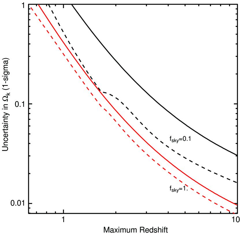
Figure 2: Uncertainties obtained on $\Omega_{k}$ are plotted vs the maximum redshift for which weak lensing cross-correlation and baryon acoustic oscillation data are jointly obtained. These are purely metric constraints on $\Omega_{k}$, and it is presumed that the WL data constrain all forms of variation of $\Omega_{k}$ except the principle degeneracy described in the text. The upper two curves are for 10% sky coverage, the lower two for full-sky. In each pair the solid line is for WL$+$BAO constraints, and the dashed line shows the effect of adding 1% measures of supernova distances in each $\Delta z=0.1$ bin for $0.4<z<1.7$.

Figure 2 also plots the $\Omega_{k}$ limits that result from combining the transverse BAO distance measurements with a supernova survey that yields independent 1% measurements of $d(z)$ at $\Delta z=0.1$ steps in the range $0.4\leq 1.7$. We find that the SN data can cut $\sigma_{k}$ in half for a transverse BAO survey with $f_{\rm sky}=0.1$, but the SN data are of only slight help (20%) to a full-sky photo-$z$ BAO survey.

We note that the Fisher uncertainties on $\Omega_{k}$ are quite independent of the number of redshift shells or of any regularization constraint on the bias factor. They are also essentially independent of the assumed proxy correlation coefficient $r$ or the WL shape noise $\sigma_{\gamma}$, because the nominal WL survey is already reducing the errors to insignificance in any mode for which it has power at all. The galaxy distribution parameters $z_{0}$ and $n$ are important only in that they have been used to determine the redshift range over which sample-variance-limited BAO data are available. If we scale back to $z_{0}=1.0$, $n=40\,{\rm arcmin}^{-2}$, as might be expected for a deep ground-based survey (Bernstein, 2005), then the uncertainty in $\Omega_{k}$ triples to $0.12f_{\rm sky}^{-1/2}$ for the nominal $\sigma_{\ln z}=0.04$ because the galaxy density drops below the BAO sample-variance limit at $z<3$. In a real survey, the distribution of galaxies with accurately measured shapes will not, however, equal the distribution of those with accurately measured photometric redshifts, so a more detailed analysis is required in order to compare surveys. It is clear, however, that sky coverage, photo-$z$ accuracy, and redshift range of joint CCC-BAO data are the key characteristics for this geometric constraint of $\Omega_{k}$.

3.2 Effects of Systematic Errors

The WL CCC method depends upon measuring shear to very high accuracy. Indeed the cosmology dependence of shear is so subtle that Mandelbaum et al. (2005) reverse the technique, and use the redshift dependence of galaxy-shear correlations as a test for systematic errors in shear measurement. Any such shear systematics could substantially degrade the curvature constraints derived above. But we show here that the CCC data will be rich enough to solve simultaneously for cosmology and calibration systematics.

The WL cross-correlation technique is insensitive to spurious shear signals caused by PSF ellipticities, because they will not correlate with the proxy mass fields. Calibration errors on the shear will, however, be important. We examine a model, similar to that of Ishak et al. (2004), in which the shear on source shell $s$ is mismeasured by a factor $(1+f_{s})$. This is simply incorporated into our governing equations by setting

$$G_{s\ell}=(1+f_{s}){d_{s}-d_{\ell}\over d_{s}}(1-\Omega_{k}d_{s}d_{\ell}/2)$$ (64)

for $d_{s}>d_{\ell}$. The Fisher matrix now has the parameters $f_{i}$ as well. We assume a Gaussian prior distribution on the $f_{i}$ for which they are all independent, with ${\rm Var}f_{i}=\sigma^{2}_{f}$.

We find the constraints on $\Omega_{k}$ from the canonical survey are essentially unchanged if $\sigma_{f}\lesssim 0.01f_{\rm sky}^{-1/2}$, a level that is probably achievable from ground or space observations. For $\sigma_{f}=1$, i.e.  complete ignorance of the calibration, $\sigma_{k}$ rises to 0.067 for the full-sky survey. The degradation in the curvature constraint is mild because even a “self-calibrated” CCC survey constrains the non-degenerate modes fairly well, and the nature of the degeneracies is only slightly expanded by the additional free parameters. A strictly $z_{s}$-dependent calibration error does not appear to be a problem for the curvature measurement.

4 Parametric Modelling

The Fisher matrix constructed over parameters $d_{i}$ and $\Omega_{k}$, marginalized over the nuisance parameters, fully describes the cosmological information content of a CCC survey. Distance information from transverse BAO and supernovae can be summed into the same matrix. If we now consider each $d_{i}$ to correspond to a known redshift $z_{i}$ (which was unimportant to the metric curvature determination), this Fisher matrix describes our knowledge of the expansion history, and can be used to forecast constraints on parametric models of the expansion of the Universe. To project the $d$–$\Omega_{k}$ Fisher matrix onto some parameters $p_{i}$, we simply need to know $dD_{A}(z)/dp_{i}$. Calibration errors on the shear can be included as described above; biases $\Delta z_{p}(z)$ in the photometric redshift scale are also easily included as they give rise to perturbations in the measured distances equal to $[d(d_{i})/dz]\,\Delta z_{p}(z)$.

The distance-based analysis is also useful in that it has revealed the nature of the constraints from the various methods. The WL cross-correlations are completely blind to changes in $\log d$ that are quadratic (linear) in $d$ when $\Omega_{k}$ is free (fixed), but offer very strong limits on any other forms of variation in $d(z)$. When WL is used in combination with transverse BAO and/or supernova measurements, the latter will serve primarily to constrain these low-order degeneracies.

As an example we consider a model for the expansion in which the free parameters are $\Omega_{k}$, $\Omega_{m}$, and the parameters $w_{0}$ and $w_{a}$ for the dark energy equation of state $w=w_{0}+w_{a}(1-a)$. Note that $\Omega_{\rm DE}=1-\Omega_{m}-\Omega_{k}$. We will also quote the uncertainty in $w_{p}$, the equation of state at the “pivot redshift” $z_{p}=1/a_{p}-1$ for which the model $w=w_{p}+(a_{p}-a)w_{a}$ has uncorrelated Fisher errors in $w_{p}$ and $w_{a}$. We consider the constraints that arise from our canonical survey of weak lensing cross-correlations and photo-$z$ BAO data. We presume a fiducial proxy-mass correlation coefficient of $r=0.7$. Table 1 lists the Fisher-matrix estimates of the standard deviations on these four parameters. Figure 3 plots error ellipses in the $w_{0}$–$w_{a}$ plane after marginalization over the other two variables.

Table 1: CCC$+$BAO Constraints on Cosmological Parameters

Photo-$z$ Error	Calibration Prior	Parameter Errors
$\sigma_{\ln z}$	$\sigma_{f}$	$\sigma(\Omega_{k})$	$\sigma(\Omega_{m})$	$\sigma(w_{p})$	$\sigma(w_{a})$
CCC only	$\cdots$	0.36	0.60	0.018	2.0
CCC only	$\cdots$	$\cdots$	0.015	0.017	0.081
0.04	$\cdots$	0.0066	0.0045	0.013	0.057
0.04	$\cdots$	$\cdots$	0.0038	0.010	0.052
0.04	0.03	0.013	0.007	0.044	0.100
0.04	0.03	$\cdots$	0.007	0.026	0.083

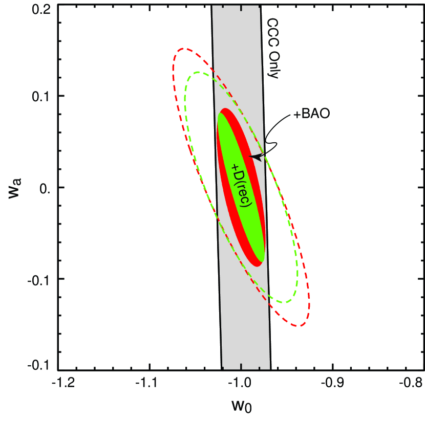
Figure 3: Error ellipses in the $w_{0}$–$w_{a}$ plane for parametric models of dark energy that have been marginalized over $\Omega_{m}$ and $\Omega_{k}$. These are 68% CL regions ($\Delta\chi^{2}=2.3$), for full-sky coverage; errors scale as $f_{\rm sky}^{-1/2}$. The large ellipse is for WL CCC information only. The middle shaded ellipse (red) adds transverse baryon acoustic oscillation data from the photo-$z$ information of the WL survey. The innermost (green) shaded region includes a measurement of the distance to recombination from expected CMB data. The two dashed ellipses allow for systematic shear calibration errors of 3% per redshift bin, which is in the “self-calibration” regime. The outer ellipse is CCC$+$BAO, the inner adds the recombination distance.

We find first that the WL CCC alone retains a strong degeneracy between $\Omega_{k}$ and the other parameters, with large errors of 0.36, 0.60, and 2.0 on $\Omega_{k}$, $\Omega_{m}$, and $w_{a}$, respectively, but with correlation coefficients $>0.99$ among all of these. [These are for full-sky surveys; we will omit the factor $f_{\rm sky}^{-1/2}$ for brevity here.] The degeneracy is broken either by assuming a flat Universe, by using the CMB distance to recombination, or by incorporating the transverse BAO information over the same sky fraction. In the last case, $\Omega_{k}$ has uncertainty 0.007, which as expected is a much tighter constraint than the model-independent one above. We also note that the $w_{p},w_{a}$ uncertainties of (0.013, 0.057) are only slightly reduced by assuming flatness, although their $z_{p}$ shifts.

Inclusion of an accurate (0.1%) angular-diameter distance to recombination from the CMB, as might be expected from Planck, drops uncertainties on $\Omega_{k}$ by a factor 3, and a factor 2 for $w_{p}$.

4.1 Scaling with Survey Characteristics

The BJ04 analysis asserts that CCC constraints improve without bound as $n^{-1/2}$. ZHS did not concur, and we would now agree. Since Stebbins (private communication) proves that ${\bf G}$ must be non-singular in the continuum limit (and we have constructed its inverse), then the matrix ${\bf K}={\bf N}+{\bf GC_{u}G}^{T}$ will remain non-singular as the shape noise ${\bf N}\rightarrow 0$, meaning that the Fisher information in Equation (56) remains finite. As a practical matter, we find that in the range of $n$ accessible to planned observations, CCC Fisher information scales only slightly more slowly than $n^{-1/2}$. There is no simple scaling once we combine the CCC information with that from BAO. The constraints are nearly independent of the choice of $\delta\Omega$, again because the shape noise dominates sample variance.

The BJ04 derivation also leads to CCC-only parametric uncertainties that scale nearly inversely with the fiducial correlation coefficient $r$. In the present analysis we see that such scaling arises if we consider only the effect of $r$ upon the ${\bf C_{g}}$ factor of Equation (57), and if we drop the left-hand term entirely. But if the effect of $r$ upon the ${\bf C_{u}}$ terms in the noise matrix ${\bf K}$ are also considered, then the dependence is more complex. We find that the CCC-only parametric constraints on flat Universes scale more weakly than inversely with $r$ over the range 0.3–1.0. The dependence is yet weaker once we include the BAO information.

4.2 Effects of Calibration Errors

Figure 4 plots the degradation of the parametric cosmology constraints as we weaken the prior on the calibration factors $f_{i}$. There are three regimes: when the calibration is known a priori to better than $\approx 10^{-3}f_{\rm sky}^{-1/2}$, there is no significant degradation due to calibration errors. Over the range $10^{-3}f_{\rm sky}^{-1/2}<\sigma_{f}<0.01f_{\rm sky}^{-1/2}$, the constraints continually degrade. Calibration uncertainties above $\approx 0.01f_{\rm sky}^{-1/2}$, however, cause no further degradation in cosmological constraints, as the CCC data solve for the systematic factors in a “self-calibration” regime. The self-calibration regime has parameter errors that are 1.6–2 times larger than the no-systematic regime. We conclude that lowering the calibration errors from 0.01 to 0.001 is equivalent to increasing the survey area by a factor of 2.5–4, but interesting cosmological constraints are possible even with poor a priori calibration systematics.

We find a similar scaling of uncertainties with calibration systematics for a shallower, ground-based survey.

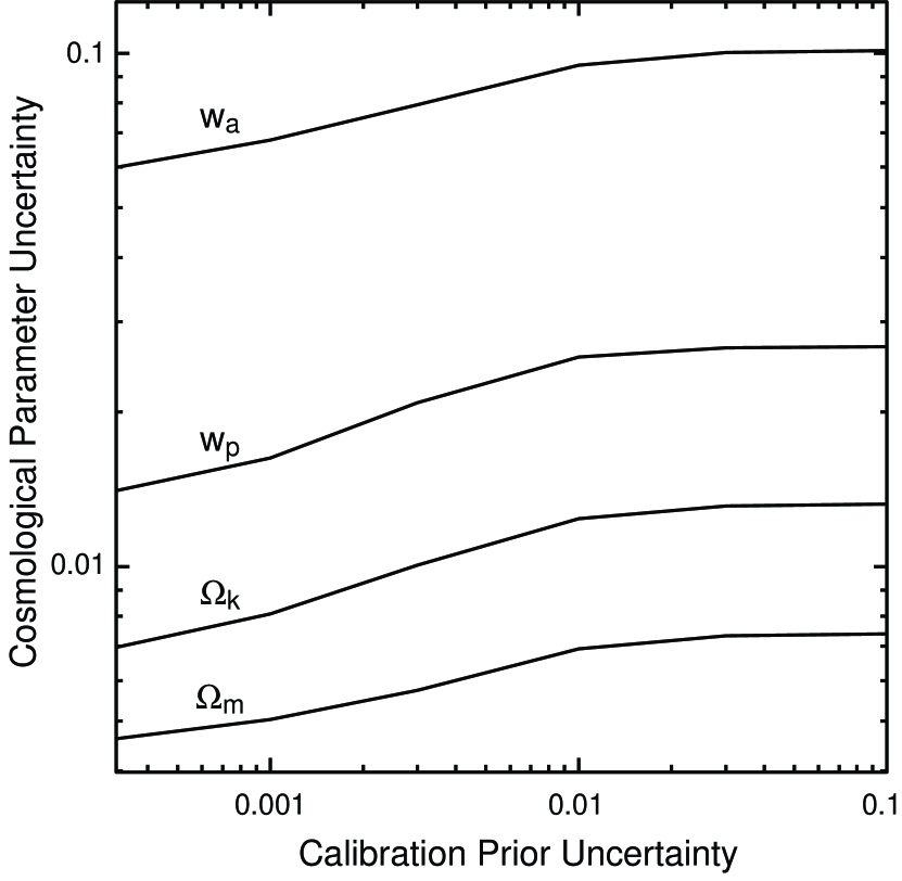
Figure 4: The 1-$\sigma$ uncertainties in each of the labelled cosmological parameters in a CCC$+$BAO survey are plotted vs the accuracy of our prior knowledge of the shear calibration factor $f_{i}$ in each redshift bin. We see that calibration errors smaller than $\approx 10^{-3}f_{\rm sky}^{-1/2}$ are harmless, and there is a “self-calibration” regime for $\sigma_{f}>0.01f_{\rm sky}^{-1/2}$, in which the CCC data solve for the calibration factors to an accuracy that is better than the prior. The degradation from self-calibration is mild. Both axes may be scaled jointly with $f_{\rm sky}^{-1/2}$.

4.3 Comparison to Previous Work

We alter the parameters of our fiducial survey to match those of ZHS, namely we set $f_{\rm sky}=0.1$, $z_{0}=1.0$, $\sigma_{\gamma}=0.3/\sqrt{2}$, $\Omega_{k}=0$, and we use an equation of state $w=w_{0}+w^{\prime}z$ instead of the $w_{a}$ form. The ZHS analysis also allows for an arbitrary distribution of mass redshift within a shell, and accounts for the signal attenuation due to photo-$z$ errors. We compare to their $\sigma_{z}=0.01$ case. For a fixed-$w$ model with only CCC information, we obtain standard deviations on $(\Omega_{m},w)$ of (0.028, 0.046) for $r=0.7$, roughly $2\times$ smaller than ZHS derive. We must lower $r$ to $0.25$ to obtain similar results. They also derive errors on $(w_{0},w^{\prime})$ when marginalized over $\Omega_{m}$ with a prior of 0.03. In this case our $r=0.7$ constraints of (0.03,0.11) compare to their (0.07,0.09)—similar in size but different in shape.

The agreement to within factor two must be considered adequate at this time. While there remain substantial differences in the analytical approach to the CCC method, the discrepancies could easily be attributed to different assumptions about the correlation between the mass and the proxy field. ZHS, as well as Hu & Jain (2004), take the galaxy distribution itself as the proxy field, and assume that the galaxies populate the mass via a pure Poisson process. In this case the correlation coefficient between multipole $l$ of the proxy and mass fields at distance $D_{A}$ is

$$r=\left\{1+\left[{dN\over dV}P(l/D_{A})\right]^{-1}\right\}^{-1/2},$$ (65)

where $P(k)$ is the 3-dimensional mass power spectrum. Thus when $nP<1$, $r$ drops below the 0.7 value of our fiducial model. This occurs at $l\gtrsim 10^{4}$ in our fiducial model for $0.5<z<2$, whereas our fiducial model makes use of shear power to higher $l$. Were we to adopt a Poisson model our parametric dark energy constraints would weaken. It is not clear, however, that the Poisson model is appropriate once we approach the length scales of group- and galaxy-scale halos, which are currently suspected of harboring a single central galaxy with near-unity probability, plus satellites. The galaxy–mass covariance on small scales may thus be a good deal stronger than Poisson models predict. This is surely a subject for further research.

We may also compare to the CCC-only results with the BJ04 method by reverting to the parameters assumed therein for the “SNAP” case: $f_{\rm sky}=0.025$, $r=0.8$, $\sigma_{\gamma}=0.15$, $\Omega_{k}=0$, and a prior of 0.03 on $\Omega_{m}$. We find a pivot redshift $z_{p}$ and uncertainty $\sigma(w_{p})$ that are the same in both cases, but $w_{a}$ is 35% lower with the present Fisher matrix. This could be a result of some of the simplifications made by BJ04 in construction of the covariance matrix for the $X_{s\ell}$ in Equation (41). Alternatively it could derive from our present assumption that the convergence, mass, and proxy field values have a multivariate Gaussian distribution, while BJ04 have the less restrictive assumption that the $X_{s\ell}$ have a Gaussian distribution.

A close comparison with Hu & Jain (2004) is well beyond our present scope, because these authors include a parametric model for the bias function and limit the cross-correlation information to multipoles $\ell<3000$. In principle both differences can be accommodated in the present formalism, by switching to a spherical-harmonic decomposition, and by projecting parametric bias constraints onto the $\Omega_{k}$–$d_{i}$–$B_{i}$ Fisher matrix before marginalizing over the $B_{i}$. A WL CCC survey reduces the errors on $\ln B$ to $\lesssim 10^{-3}f_{\rm sky}^{-1/2}$, apart from a quadratic degeneracy with distance. Hence the a priori theoretical constraints would need to be stronger than this in order to improve dark energy measurements. We also note that Hu & Jain take a Poisson model for the mass-galaxy correlation, and assume a density of lens galaxy samples that is 2 orders of magnitude lower than assumed here, which we believe accounts for the cross-correlation constraints being much weaker in that work than in the present calculations.

A short summary of this subsection is that there are currently multiple formalisms for analysis of CCC data, and they currently differ by up to a factor 2 in Fisher uncertainties on parametric dark-energy models. Further work is certainly required in order to understand the nature of the CCC constraints, and to understand our ability to reconstruct the mass distribution from the galaxy data.

5 Discussion

Reparameterizing the observable galaxies by their (dimensionless) angular diameter distance $d$ rather than redshift $z$ makes it clear how the WL CCC method can provide model-independent geometric constraints on $\Omega_{k}$. This methodology also reveals that CCC data is degenerate under alterations to $\ln b$ and $\ln d$ by quadratic functions of $d$, if $\Omega_{k}$ is free. Apart from three exact degeneracies, the cross-correlation strength, being a joint function of the lens and source distances, is very efficient at producing decoupled estimates of $\Omega_{k}$, the distances $d_{i}$ and the bias factors $B_{i}$, and can even determine shear calibration factors $f_{i}$ for each source plane with modest degradations of factor $\lesssim 2$ in cosmological accuracy.

With sufficiently accurate photometric redshifts, the same survey data used for weak lensing may be used to determine the transverse BAO scale. This gives additional model-independent constraints on $d$ that are of lower precision than the CCC data, but are completely free of degeneracy. Such a combined CCC-BAO survey should yield uncertainties of $\approx 0.04f_{\rm sky}^{-1/2}$ on $\Omega_{k}$. We reiterate that such constraints are completely independent of any assumptions about the matter-energy content of the Universe, any biases in photometric redshifts, or in fact any alterations to the Friedmann equations or the deflection equations for light. They merely require that the Robertson-Walker metric be applicable to our Universe. Given the lack of viable dark-energy theories, it seems prudent to seek cosmological information that remains valid even if the acceleration is attributable to an alteration of General Relativity rather than a previously unnoticed stress-energy contribution.

In the spirit of conservatism, we should note that the RW metric may not be sufficiently accurate. The clumpiness of the matter-energy distribution may invalidate our adoption of the filled-beam angular diameter distance, and a more sophisticated treatment may be required (Holz & Linder, 2004). It is not clear to what extent small-scale clumpiness can influence the apparent shear of galaxy-scale images as surveyed across the entire sky—this is quite a different regime from studies of strongly lensed quasars or supernovae for which the Dyer-Roeder distances have been most carefully studied.

The curvature measurement is limited by the ability to break the WL CCC degeneracy, i.e.  by the accuracy and redshift span of the BAO or SN measurements of angular-diameter distances. Our baseline constraint assumes photo-$z$ BAO information for $0<z<3$ over the full sky. A massive spectroscopic BAO survey would offer substantial improvement, but Type Ia supernova studies would not offer substantial improvement over full-sky photo-$z$ BAO unless systematic uncertainties in SNIa peak magnitudes could be brought well below 1% and the redshift range extended beyond $z=2$. Inclusion of lensing and acoustic-scale information from the epochs of recombination or reionization would help significantly.

The parametric dark-energy constraints derived from the CCC$+$BAO information are more fluid, as our derivation has made somewhat arbitrary assumptions about the correlation between the true mass and the proxy mass derived from the galaxy distribution. The simplifying assumptions about Gaussianity, uncorrelated mass shells, and uncorrelated lines of sight should also be improved upon. The spherical-harmonic-based Fisher analyses of Hu & Jain (2004), Song & Knox (2004), and ZHS are in this respect superior to our treatment of uncorrelated lines of sight. We note however that the Fisher matrix from Equation (56) is applicable to multipole coefficients. More work is also required to examine the impact of finite photo-$z$ precision on the CCC constraints, as per ZHS.

A weak lensing survey would produce other kinds of information which we have not used in this analysis. Power-spectrum (Hu, 1999; Refregier et al., 2004) and bispectrum (Takada & Jain, 2004) tomography, and WL cluster counts (Weinberg & Kamionkowski, 2003; Marian, & Bernstein, 2005) constrain dark energy once a model for the growth of structure $G(z)$ is specified. One could augment our current $\Omega_{k}-d_{i}$ Fisher matrix with growth factors $G(d_{i})$ to produce a non-parametric information estimate, which could then be projected onto the parameters of specific models, even those which predict changes to the usual equation for linear growth of perturbations in an expanding Universe.

The method proposed herein for metric constraints on curvature, and for strong parametric constraints on cosmology, will require substantial practical advances before implementation, plus additional theoretical work. Progress in high-accuracy shape and photo-$z$ measurement is needed, as is research into intrinsic galaxy-shape correlations (Hirata & Seljak, 2004), non-linearities in lensing (White, 2005), and methods of reconstructing the matter distribution from a galaxy distribution. Nonetheless the WL CCC method shares with the BAO method the ability to generate extremely robust and model-independent cosmological constraints, particularly when they are used in combination.

References

- Bernstein (2005) Bernstein, G. 2005 (in preparation)
- Bernstein & Jain (2004) Bernstein, G. & Jain, B., 2004, ApJ, 600, 17 [BJ04]
- Eisenstein et al. (2005) Eisenstein, D. J. et al., 2005
- Glazebrook & Blake (2005) Glazebrook, K. & Blake, C., 2005, ApJ, (submitted)
- Gautret, Fort, & Mellier (2000) Gautret, L., Fort, B., & Mellier, Y. 2000, A&A, 353, 10
- Golse, Kneib, & Soucail (2002) Golse, G., Kneib, J.-P., & Soucail, G. 2002, A&A, 387, 788
- Hirata & Seljak (2004) Hirata, C. M., & Seljak, U. 2004, Phys. Rev. D, 70, 063526
- Holz & Linder (2004) Holz, D. & Linder, E. V. 2004, astro-ph/0412173
- Hu (1999) Hu, W. 1999, ApJ, 522, L21
- Hu & Jain (2004) Hu, W, & Jain, B., 2004, Phys. Rev. D, 70, 043009
- Ishak et al. (2004) Ishak, M., Hirata, C. M., McDonald, P., & Seljak, U. 20004, Phys. Rev. D, 69, 083002514
- Jain & Taylor (2003) Jain, B., & Taylor, A. 2003, Phys. Rev. Lett., 91, 141302
- Jimenez et al. (2003) Jimenez, R., Verde, L., Treu, T., & Stern, D. 2003, ApJ, 593, 622
- Linder (1988) Linder, E. V. 1988, A&A, 206, 175
- Link & Pierce (1998) Link, R. & Pierce, M. J. 1998, ApJ, 502, 63
- Luminet et al. (2003) Luminet, J., Weeks, J. R., Riazuelo, A., Lehoucq, R., & Uzan, J. 2003, Nature, 425, 593
- Mandelbaum et al. (2005) Mandelbaum, R. et al. 2005, astro-ph/0501201
- Marian, & Bernstein (2005) Marian, L., & Bernstein, G. 2005 (in preparation)
- Massey et al. (2004) Massey, R., et al. 2004, AJ, 127, 3089
- Peebles (1993) Peebles P J E, 1993 Principles of Physical Cosmology (Princeton, NJ: Princeton University Press)
- Pen (2004) Pen, U.-L., 2004, New Astronomy 9, 417
- Refregier et al. (2004) Refregier, A., et al. 2004, AJ, 127, 3102
- Seo & Eisenstein (2003) Seo, H.-J. & Eisenstein, D. J. 2003, ApJ598, 720
- Sereno (2002) Sereno, M. 2002, A&A, 393, 757
- Song & Knox (2004) Song, Y.-S. & Knox, L. 2004,
- Soucail et al. (2004) Soucail, G., Kneib, J.-P., & Golse, G. 2004, A&A, 417, L33
- Spergel et al. (2003) Spergel, D. N., et al. 2003, ApJS, 148, 175
- Stebbins (2005) Stebbins, A. 2005 (private communication)
- Takada & Jain (2004) Takada, M., & Jain, B. 2004, MNRAS, 348, 897
- Tegmark, Taylor, & Heavens (1997) Tegmark, M., Taylor, A., Heavens, A., 1997, ApJ, 480, 22
- Uzan, Kirchner, & Ellis (2003) Uzan, J.-P., Kirchner, U., & Ellis, G. F. R. 2003, MNRAS344, L65
- Weinberg (1970) Weinberg, S. 1970, ApJ, 161, L233
- Weinberg & Kamionkowski (2003) Weinberg, N. N., & Kamionkowski, M. 2003, MNRAS, 341, 251
- White (2005) White, M. 2005, astro-ph/0502003
- Zhang, Hui, & Stebbins (2003) Zhang, J., Hui, L., & Stebbins, A. 2003, astro-ph/0312348 [ZHS]