Effects of a solid surface on jet formation around neutron stars

We present two numerical simulations of an accretion flow from a rotating torus onto a compact object with and without a solid surface – representing a neutron star and a black hole – and investigate its influence on the process of jet formation. We report the emergence of an additional ejection component, launched by thermal pressure inside a boundary layer (BL) around the neutron star and examine its structure. Finally, we suggest improvements for future models.

1 Introduction

Although jets are ubiquitous phenomena in many different astrophysical objects, their formation is relatively unclear. We find jets in young stellar objects where they are driven by protostars, in symbiotic stars (white dwarfs), X-ray binaries (neutron stars and stellar mass black holes) and active galactic nuclei (supermassive black holes). The mass loss rate of all jets is found to be connected to the mass accretion rate of the underlying disk found in most objects (e.g. Livio 1997). Therefore the necessary components seem to be well known and common to all objects.

In jet formation models presented so far, the magnetic field seems to play a key role. The first analytical work studying magneto-centrifugal acceleration along magnetic field lines threading an accretion disk was done by Blandford & Payne (1982). They have shown braking of matter in azimuthal direction inside the disk and its acceleration above the disk surface by the poloidal magnetic field components. Toroidal components of the magnetic field then collimate the flow. Numerous semi-analytic models extended the work of Blandford & Payne (1982), which either were restricted to self-similar solutions and their geometric limitations (e.g. Pudritz & Norman 1986; Vlahakis & Tsinganos 1998, 1999; Ferreira & Casse 2004) or suggested non-self-similar solutions (e.g. Camenzind 1990; Pelletier & Pudritz 1992; Breitmoser & Camenzind 2000).

Another approach is to use time-dependant numerical MHD simulations to investigate the formation and collimation of jets. In most models, however, a polytropic equilibrium accretion disk was regarded as a boundary condition (e.g. Krasnopolsky, Li & Blandford 1999, 2004; Anderson et al. 2004; Goodson, Böhm & Winglee 1999). The magnetic feedback on the disk structure is therefore not calculated self-consistently. Only in recent years were the first simulations presented including the accretion disk self-consistently in the calculations of jet formation (e.g. Casse & Keppens 2002, 2004; Kato, Mineshige & Shibata 2004).

Pringle (1989) proposed the idea of jet formation in the BL region and also in his model strong magnetic fields were driving the outflows. Torbett (1984) first assumed the liberation of energy in BL shocks to drive winds by thermal pressure. Livio (1999) pointed out that an additional source of energy beside the magnetic one is needed to power jets. Torbett & Gilden (1992) performed numerical simulations and found mass ejection only when they had not taken radiative cooling into account. However, their simulations were only one-dimensional for calculating the vertical structure of the BL. New examinations and modifications of this possibility of accelerating plasma close to the central object were done by Soker & Regev (2003) involving SPLASHs (SPatiotemporal Localized Accretion SHocks) in the BL. Locally heated bubbles expand, merge, and accelerate plasma to higher velocities than the local escape velocity. This scenario was introduced in analytic estimates. Now the numerical treatment needs to be improved using multi-dimensional simulations – at first purely hydrodynamical ones, which are presented in this paper.

In Sect. 2, we present our numerical simulations of an accretion flow onto a neutron star with a solid surface and onto an accreting black hole without one, with which we investigate its effects on the jet formation process (Sect. 3). Sections 4 and 5 examine the structure of the accretion flow and of the additional ejection component, while a discussion follows in Sect. 6.

2 The numerical models

In the following, we describe our computer code with equations, the model geometry, and the parameters.

2.1 The computer code

With the code NIRVANA (Ziegler 1998, 1999) we solve the following set of differential equations of ideal non-relativistic magnetohydrodynamics

$$\frac{\partial\,\rho}{\partial\,t}+\nabla\,(\rho\,{\bf v}) = 0$$

$$\frac{\partial\,(\rho\,{\bf v})}{\partial\,t}+\nabla\,(\rho\,{\bf v}\otimes{\bf v}) = -\nabla\,p+\frac{1}{\mu}\,(\nabla\times{\bf B})\times{\bf B}-\rho\,\nabla\Phi$$

$$\frac{\partial\,e}{\partial\,t}+\nabla\,(e\,{\bf v}) = -p\,\nabla\,{\bf v}$$

$$p = (\gamma-1)\,e$$

$$\frac{\partial\,{\bf B}}{\partial\,t} = \nabla\times({\bf v}\times{\bf B})$$ (1)

with density $\rho$, velocity ${\bf v}$, internal energy $e$, pressure $p$, magnetic field ${\bf B}$, gravitational potential $\Phi$, magnetic permeability $\mu$, and adiabatic constant $\gamma$.

A set of common boundary conditions, including inflow, outflow (open), mirror and anti-mirror and rotational symmetry, all with their usual meanings, has already been defined in NIRVANA. The code and its boundary conditions were tested in many simulations (Ziegler 1998, 1999, and references therein).

2.2 Initial conditions

Besides taking the more or less standard disk as initial condition, another approach is to begin with a rotating torus inside the computational domain. One advantage of this setup is that all material is already inside the domain initially, so no matter source has to be implemented on the boundaries. In this case, we could use the standard boundary conditions of NIRVANA.

Starting with the static hydrodynamics equations, from the momentum equation follows

$$\frac{1}{\rho}\,\nabla\,p=-\,\nabla\,\Phi+\frac{l^{2}}{r^{3}}\,\nabla\,r,$$ (3)

where $r$ is the cylindrical radius. With a polytropic equation of state and the identity

$$\nabla\,(\frac{p}{\rho})=\frac{\gamma-1}{\gamma}\,\frac{1}{\rho}\,\nabla\,p$$ (4)

Eq. (3) can be integrated to

$$\frac{\gamma}{\gamma-1}\,\frac{p}{\rho}+\Phi+\int_{r}^{\infty}\,dr^{\prime}\,\frac{l(r^{\prime})^{2}}{r^{\prime 3}}=W_{0}.$$ (5)

Under the assumption of constant $l$, the integral can be solved to

$$\frac{\gamma}{\gamma-1}\,\frac{p}{\rho}+\Phi+\frac{1}{2}\,\frac{l^{2}}{r^{2}}=W_{0}$$ (6)

with which the density is then

$$\rho=\left(\frac{1}{\kappa}\,\frac{\gamma-1}{\gamma}\,\left[W_{0}-\Phi-\frac{1}{2}\,\frac{l^{2}}{r^{2}}\right]\right)^{1/(\gamma-1)}.$$ (7)

The angular momentum of the torus is then dependent on its radial position $R_{0}$ as

$$l(R_{0})=\sqrt{G\,M\,R_{0}}\,\frac{R_{0}}{R_{0}-2\,R_{\rm g}},$$ (8)

if a pseudo-Newtonian gravitational potential (Paczynski & Wiita 1980)

$$\Phi=-\frac{G\,M}{R-2\,R_{\rm g}}$$ (9)

is chosen. $R$ is the spherical radius, and all distances are now given in units of $R_{\rm g}$. The corresponding time scale $t_{0}$ is then the inverse of the Keplerian period $t_{0}\approx 10^{-4}$ s in our simulations. The density maximum of the torus was positioned to 8 $R_{\rm g}$.

Inside the torus, the velocity components are then

$$v_{\phi}=\frac{l(R_{0})}{r}\qquad v_{r}=v_{\theta}=0.$$ (10)

Outside the torus, Keplerian rotation is assumed

$$v_{\phi}=\Omega_{\rm K}\,r\qquad v_{r}=v_{\theta}=0$$ (11)

with

$$\Omega_{\rm K}=\sqrt{G\,M\,R}\,\frac{R}{R-2\,R_{\rm g}}\,\frac{1}{r^{2}}.$$ (12)

To initialise the magnetic field and to assure that its divergence vanishes, we calculate the magnetic field components from the vector potential $\@vec{A}$ defined as

$$\@vec{B}=\nabla\,\times\,\@vec{A}.$$ (13)

The only considered component of $\@vec{A}$ is set identical to the internal energy

$$A_{\phi}=e.$$ (14)

The initial magnetic field lines are then along isocontours of energy and density, as we used a polytropic equation of state during initialisation. This results in the following magnetic field components

$$B_{R}=\frac{1}{R\,\sin{\theta}}\,\frac{\partial}{\partial\,\theta}\,(\sin{\theta}\,e)\quad B_{\theta}=-\frac{1}{R}\,\frac{\partial}{\partial\,R}\,(R\,e)\quad B_{\phi}=0$$ (15)

in spherical coordinates, or

$$B_{r}=-\frac{\partial}{\partial\,z}e\qquad B_{z}=\frac{1}{r}\,\frac{\partial}{\partial\,r}\,(r\,e)\qquad B_{\phi}=0$$ (16)

in cylindrical coordinates. Afterwards, these components were scaled to achieve an assumed plasma $\beta=p_{\rm gas}/p_{\rm mag}=10^{3}$. Note that no global external magnetic field was implemented.

We performed two simulations with different boundary conditions at the inner radial coordinate, one with open boundaries (Run A) – describing a black hole – and one with anti-mirror conditions to model the solid surface of the central object (Run B) – a neutron star. The other boundary conditions are open ones at the outer radial coordinate, rotation symmetry and anti-mirror symmetry at the inner and outer poloidal ($\theta$-) coordinate, respectively, to simulate the rotational axis and the equatorial plane, and periodic conditions at both azimuthal ($\phi$-) boundaries. The aim of these simulations was to investigate the influence of the solid surface. A third simulation (Run C) was performed similar to Run A, but in cylindrical coordinates to investigate the influence of different coordinate systems. Here the cylindrical radius starts at $2\,R_{\rm g}$; i.e. a cylinder along the axis is cut out and the inner radial boundary is chosen to be open.

3 The effect of a solid surface on the jet formation process

3.1 The accretion and ejection components

In Fig. 1, the logarithm of density is plotted for the three runs after 45 $t_{0}$. One can clearly see that activity is triggered much faster in Run B with the solid surface boundary.

In Run A accretion sets in immediately because of the magneto-rotational instability (Balbus & Hawley 1998) inside the torus. After almost one revolution of the torus, it comes in contact with the central object, which leads to a re-distribution of matter in the now established disk. The inner part of the disk puffs up creating an expanding bubble. Along the rotation axis, a funnel – i.e. a region evacuated by centrifugal forces to densities that are three orders of magnitude below the surrounding – is created and its cross-section grows with time.

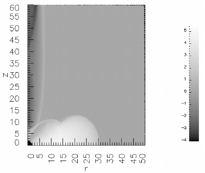
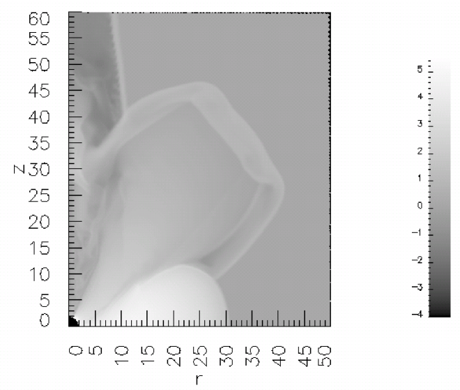
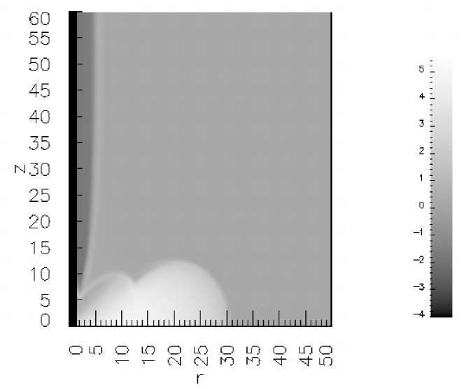
Figure 1: Plots of the logarithm of density of Run A (top), Run B (middle) and Run C (bottom) after 45 $t_{0}$; the coordinates are in units of $R_{\rm g}$

In Run B the accretion process also starts immediately and the funnel is created. Additionally, a boundary layer with a radial extent of one fifth of the inner radius forms on the surface of the central object. Due to its high pressure, a flare occurs. This flare bubble, now created by the boundary layer and not by the accretion disk, expands along the surface of the torus with high velocities and high density. The density contrast of the bubble is $\eta=10^{2}$, i.e. the bubble is overdense. Expansion of this bubble is powered by a continuous high pressure flow from the boundary layer. The expansion direction of the bubble is along a latitude of around 40-50^∘. If an external magnetic field were present, perhaps the flow would bend towards the axis.

Only in Run C, a high velocity component emanates out of the spherical expansion inside the swept-out funnel along the axis after 64.5 $t_{0}$. This funnel jet has a head velocity between $c/3$ and $c$ and a density contrast of $\eta=10^{-2}$. As this is only seen in Run C and not in Run A, the open boundary might create this feature.

Figure 2: Time evolution of accretion rate $\dot{M}=-4\,\pi\,\rho\,v_{r}\,H$ in the equatorial plane at $r=4\,R_{\rm g}$. In Run C the accretion rate is always higher than in the other simulations, perhaps due to the boundary conditions. After 21 $t_{0}$, the flare coming from the boundary layer destabilizes the accretion flow and increases its rate in Run B.

In Fig. 2, the time evolution of the accretion rate in the equatorial plane at $r=4\,R_{\rm g}$ is plotted. It is calculated as $\dot{M}=-4\,\pi\,\rho\,v_{r}\,H$ with height $H$ of the disk. The qualitative behavior seems to be equal in all runs, but in Run C the accretion rate is always higher. It is possible that the open boundary near the axis causes a global radial inflow which is superimposed on the accretion rate visible in Runs A and B. The accretion rate in the Runs A and B seems to be equal until about 21 $t_{0}$; i.e. no causal connection is established between the boundary layer and the accretion flow itself until then. After that point, the flare coming from the boundary layer destabilizes the accretion flow and increases its rate.

3.2 Jet emission efficiency

In Fig. 3, a poloidal slice at $r=10\,R_{\rm g}$ of the mass accretion/outflow rate – again calculated as $\dot{M}=-4\,\pi\,\rho\,v_{r}\,H$ – is plotted at different times for Run A and for Run B. One can clearly see the different accretion and ejection components in this simulation.

Figure 3: Poloidal slice at $r=10\,R_{\rm g}$ of the mass accretion/outflow rate $\dot{M}=-4\,\pi\,\rho\,v_{r}\,H$ of Runs A (top) and B (bottom) at different times. The emergence of an additional outflow component is visible at about 40^∘.

The first peak at about 40^∘ represents the flares created by the boundary layer in Run B and has no corresponding feature in Run A. The second peak at about 70^∘ is identical to an outflow along the surface of the torus, which is common in all runs. At larger values of $\theta$, the accretion flow can be seen. At this distance of $10\,R_{\rm g}$ the accretion rate is higher in Run A than in Run B, while at closer distance the behavior is reversed (Fig. 2). The accretion rate in all peaks is highly time dependent in Run B, while it seems to reach an asymptotic value in Run A (Fig. 4), which results from the flary conditions inside the BL.

Figure 4: Time evolution of the ejection peaks and the accretion disk in Run A (top) and Run B (bottom). While the accretion/outflow rates seem to reach an asymptotic value in Run A, they are highly variable in Run B due to the flary conditions inside the BL.

Using the mass accretion rate in the equatorial plane and the mass ejection rate of the two peaks, one can calculate an ejection efficiency of the system as the ratio of both rates. This efficiency is plotted in Fig. 5. After an initial phase of global ejection in the equatorial plane until about 14 $t_{0}$, the mass fraction outflowing along the torus surface (second peak) compared to that being accreted is almost constant between 25–30 % in Run A, while oscillating around a mean of about 50 % in Run B. In Run A, the efficiency of ejection in the first peak is only one percent and the ejection peak is not really present. In Run B, however, the ejection efficiency of the first peak is comparable to that of the second peak, i.e. also in the range between 40-50 %. Therefore almost the whole accreted matter is ejected out of the central region.

Figure 5: Efficiency of the ejection mechanism, calculated as the ratio of the outflow rate in the ejection peak to the accretion rate in the equatorial plane plotted for Runs A (top) and B (bottom)

4 Structure of the accretion flow

The next step is to investigate the structure of the accretion flow and to raise the question of influences of the emergence of the boundary layer. In Figs. 6-9, the main magnetohydrodynamical quantities of the flow are plotted.

Figure 6: Structure of the accretion flow after 14 $t_{0}$: density. The density increases in the BL by more than an order of magnitude with respect to the accretion flow, in Run A, the open boundary representing the inner sink arranges for a density decrease by a factor of 4-5.

Figure 7: Structure of the accretion flow after 14 $t_{0}$: ratio of angular momentum to Keplerian angular momentum. In Run B the accretion flow is always rotating super-Keplerian and the angular momentum of the flow in Run A drops below the Keplerian angular momentum for distances smaller than about 3 $R_{\rm g}$.

Figure 8: Structure of the accretion flow after 14 $t_{0}$: pressure. The thermal pressure is enhanced in Run B inside the BL by six orders of magnitude with respect to Run A.

Figure 9: Structure of the accretion flow after 14 $t_{0}$: azimuthal magnetic field component. The emergence of the boundary layer also creates a peak in the magnetic field at its surface, which is perhaps caused by compression in strong shocks inside it.

In Fig. 6,which shows the density distribution in the equatorial plane, the boundary layer between 2 and 2.4 $R_{\rm g}$ (1-1.2 radii of the central object) is, along with the torus, the most prominent feature in Run B. The density increases by more than an order of magnitude with respect to the accretion flow. In Run A, the open boundary representing the inner sink creates a density decrease by a factor of 4-5, due to draining into the black hole. In contrast to Run B, in which the accretion flow is always rotating super-Keplerian, the angular momentum of the flow in Run A drops below the Keplerian angular momentum for distances smaller than about 3 $R_{\rm g}$ (Fig. 7). This is also an effect of the drag created by the black hole. The thermal pressure is enhanced in Run B inside the BL by six orders of magnitude compared to Run A (Fig. 8). The emergence of the boundary layer also creates a peak in the radial and azimuthal components of the magnetic field (Fig. 9) at its surface, which is perhaps caused by compression in strong shocks inside it. This highly magnetised region extends to a distance of 60 $R_{\rm g}$ from the equatorial plane, leading to a positive total poloidal current instead of negative values near and inside the torus (Fig. 10), which then can also drive jets magnetically.

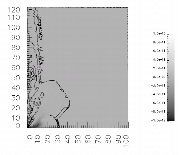
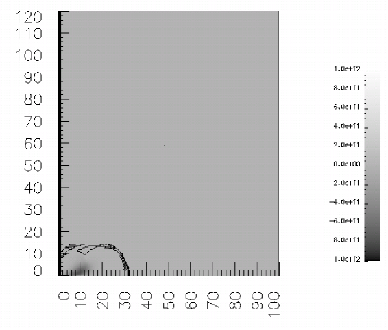
Figure 10: Plots of the total poloidal current $r\,B_{\phi}$ after 31 $t_{0}$ for Run A (top), Run B (middle) and Run C (bottom) with logarithmic contour lines from $I=0$ to $I=10^{12}$ A

5 Structure of the BL ejection component

In Figs. 11-12 the density and temperature along a slice through the ejection component at $\theta=45^{\circ}$ are plotted.

Figure 11: Structure of the ejection component at $\theta=45^{\circ}$ after 54 $t_{0}$: density. Knots with enhanced density are present.

Figure 12: Structure of the ejection component at $\theta=45^{\circ}$ after 54 $t_{0}$: temperature

The variability of the accretion and ejection rates leaves its mark in the form of a rich substructure in all variables, especially in density. One can distinguish knots with enhanced density, magnetic field components, and temperature. In the velocity components, the knots are modulated on a global deceleration of the flow. The jet is still highly transient and simulations with an extended computational domain have to show whether a steady outflow on larger scales can be established.

6 Discussion

We set up numerical simulations of a compact object with and without a solid surface accreting matter from a rotating torus. They show an additional ejection component that could be collimated into a jet by a global magnetic field which was, however, omitted in our simulations. Another possibility for achieving collimation is an external pressure gradient, which was also not present in our simuations.

Our results seem to support the SPLASH scenario of Soker & Regev (2003). We reported the emergence of a ejection component which is highly variable in agreement with their scenario. In our simulations a two-dimensional treatment was used, the full description in three dimensions could reveal new effects or details which we have to look for in new simulations.

Another point is the amount of physics in our models. We used the equations of ideal MHD neglecting any cooling effects. Depending on the accretion rate, however, the boundary layer material can become optically thick, which has to be taken into account. The additional equations in the flux-limited diffusion ansatz can no longer be solved by NIRVANA, so that a new tool has to be used e.g. FLASH, and a new branch of simulations will be necessary. As cooling effects reduce the internal energy of the material and thereby also reduce its thermal pressure, it has to be shown, whether this new jet formation scenario is still reliable in two- or three-dimensional models.

We have presented simulations with a set of model parameters appropriate for an accreting neutron star and an accreting black hole, respectively. The accretion rate in our simulations is, however, far too large for XRBs, but would only be suitable for a gamma-ray burst. These are created by an overestimated density inside the rotating torus. Further simulations need to show whether this scenario still works at lower rates and will have to fix the value of a critical accretion rate, as stated in the analytic model by Soker & Lasota (2004).

The equations of ideal MHD can theoretically be written in a non-dimensional form, if one uses a Newtonian gravitational potential instead of the pseudo-Newtonian one. Neglecting the latter, we could normalize all quantities to naturally arising combinations which depend on parameters of the central object and carry over our results to other jet sources. However, additional simulations representing other classes of jet emitting objects will follow.