Generating cosmological perturbations with mass variations

Abstract

We study the possibility that large scale cosmological perturbations have been generated during the domination and decay of a massive particle species whose mass depends on the expectation value of a light scalar field. We discuss the constraints that must be imposed on the field in order to remain light and on the annihilation cross section and decay rate of the massive particles in order for the mechanism to be efficient. We compute the resulting curvature perturbations after the mass domination, recovering the results of Dvali, Gruzinov, and Zaldarriaga in the limit of total domination. By comparing the amplitude of perturbations generated by the mass domination to those originally present from inflation, we conclude that this mechanism can be the primary source of perturbations only if inflation does not rely on slow-roll conditions.

1 Introduction

Although inflation has recently become the paradigm of the early universe and the dominant contender for generating the observed large scale density perturbations [1], it is known to be plagued by the difficulty of being embedded in most current particle physics models.

The usual hypothesis is that primordial density perturbations originate from the vacuum quantum fluctuations of the inflaton field. The fact that the inflaton has to remain light during inflation and that its vacuum energy is constrained by the amplitude of the observed cosmological perturbations make it difficult to construct motivated models [2]. For this reason, scenarios where inflation does not rely on slow-roll conditions have recently been proposed (see e.g., [3]).

If, as in these scenarios, the inflaton has no fluctuations, it is necessary to find a mechanism to generates cosmological perturbations. In the curvaton scenario [4, 5] curvature perturbations are generated by the late decay of a light scalar field $\phi$, whose fluctuation $\delta\phi$ is amplified during inflation with a quasi-scale invariant spectrum, and amplitude set by the Hubble rate at horizon crossing, $\delta\phi\sim H$. This mechanism opens up new possibilities for observations and for model building. In particular, it can liberate the inflaton from the requirement that it is responsible for the primordial perturbations.

In the same spirit, inspired by the idea that coupling constants and masses of particles during the early universe may depend on the value of some light scalar field, a number of people have proposed that perturbations could be generated from the fluctuations of the inflaton coupling to ordinary matter during reheating, a mechanism called inhomogeneous reheating or modulated fluctuations [6] (see also [7, 8] and [9, 10] for the perturbations).

Here we study the possibility that cosmological perturbations are generated during the phase of domination of a massive particle species $\psi$ whose mass is modulated by the value of a light field $\phi$, as originally proposed in [11]. These particles are produced and thermalize after inflation. If sufficiently long-lived, they can freeze out and eventually dominate the universe when they become non-relativistic. Due to the mass fluctuation, the mass domination process becomes inhomogeneous and converts the fluctuation of $\phi$ into curvature perturbations.

In [12] we studied the perturbations generated by this mechanism making use of the formalism introduced in [13] for interacting fluids. Here we take a different approach and, in particular, we consider more appropriate initial conditions for the perturbations of the massive particles after inflation. Due to this different choice of initial conditions, the result found here for the final curvature perturbation in terms of the mass fluctuations does not agree with [12], but confirms [11].

In the next section we model the inhomogeneous mass domination. We derive and discuss the conditions that must be imposed on the field for remaining light (Sec. 3) and on the annihilation cross section and decay rate of the massive particles in order for $\psi$ to dominate the universe and for the mechanism to be efficient (Sec. 4). Finally, we study the perturbations and the observational consequences of this mechanism, and we discuss when it can successfully liberate inflation.

2 Modeling the mass fluctuation

In this section we discuss the homogeneous evolution equations governing a fluid of non-relativistic particles $\psi$ with a rest mass that depends on the value of a scalar field. Since we want to describe the universe after reheating, we also add a radiation fluid and let $\psi$ to decay into radiation. The derivation given here of the coupling between $\psi$ and $\phi$ is ‘intuitive’: A more rigorous treatment can be found in the literature on scalar-tensor theories such as in [14, 15].

We consider a flat Friedmann-Lemaître-Robertson-Walker universe, with metric $ds^{2}=-dt^{2}+a^{2}(t)dx^{2}$. The Hubble rate $H=\dot{a}/a$ (${{}^{\hbox{.}}}\!=\partial/\partial t$) is given by

$$H^{2}=\frac{1}{3m^{2}_{\rm P}}(\rho_{\psi}+\rho_{\gamma}+\rho_{\phi}),$$ (1)

where $\rho_{X}$ is the energy density of the $X$ species and $m_{\rm P}=(8\pi G)^{-1/2}$ is the reduced Planck mass.

The non-relativistic particles considered here are similar to cold dark matter particles: they are collisionless and non-relativistic. Hence their pressure vanishes and their energy density is given by the product of the particle number density and the mass,

$$T_{\mu\nu}^{(\psi)}=\rho_{\psi}u_{\mu}u_{\nu}=m_{\psi}n_{\psi}u_{\mu}u_{\nu},$$ (2)

where $u_{\nu}$ is the four-velocity. The mass of $\psi$ depends on a scalar field $\phi$, $m_{\psi}=m_{\psi}(\phi)$.

We consider $\psi$ after freeze-out so that $n_{\psi}$ is not changed by annihilation processes. However, since we want to allow $\psi$ to decay into radiation, we define a decay rate of change of the number of $\psi$ particles as $\nabla_{\mu}(n_{\psi}u^{\mu})=-\Gamma n_{\psi}$. With this equation, Eq. (2) yields a conservation equation for the energy of $\psi$, written in covariant form [12],

$$u^{\nu}\nabla_{\mu}T_{\nu}^{(\psi)\mu}=-(\alpha\phi^{-1}\partial_{\mu}\phi u^{\mu}-\Gamma)\rho_{\psi},$$ (3)

where we have defined the (dimensionless) mass coupling function $\alpha={d\ln m_{\psi}}/{d\ln\phi}$. Even in the absence of coupling to radiation, due to the interaction with $\phi$, the energy of $\psi$ is not conserved.

Since $\psi$ decays only into radiation, the evolution equation governing the radiation energy density is

$$u^{\nu}\nabla_{\mu}T_{\nu}^{(\gamma)\mu}=-\Gamma\rho_{\psi}.$$ (4)

The background conservation equations for the two fluids then become (with $P_{\gamma}=\rho_{\gamma}/3$)

$$\dot{\rho}_{\psi} = -(3H-\alpha\dot{\phi}/\phi+\Gamma)\rho_{\psi},$$ (5)

$$\dot{\rho}_{\gamma} = -4H\rho_{\gamma}+\Gamma\rho_{\psi}.$$ (6)

The scalar field $\phi$ has a standard kinetic term and a potential $V(\phi)$. However, its evolution equation is sourced by an additional term due to the coupling to the bath of non-relativistic particles $\psi$. Indeed, the requirement that the sum of the three energy-momentum tensors is conserved, $\sum_{X}\nabla_{\mu}T_{\nu}^{(X)\mu}=0$, yields

$$\nabla_{\mu}\partial^{\mu}\phi=V^{\prime}+(\alpha/\phi)\rho_{\psi}.$$ (7)

The background Klein-Gordon equation for the scalar field in discussed in the following section.

3 Scalar field behavior

The background part of Eq. (7) can be rewritten as

$$\ddot{\phi}+3H\dot{\phi}+V^{\prime}=-(\alpha/\phi)\rho_{\psi},$$ (8)

where ${}^{\prime}\!=d/d\phi$. Taking into account the coupling to $\psi$, the scalar field behaves as a field in the effective potential $V_{\rm eff}(\phi)=V(\phi)+\rho_{\psi}$. The coupling can have the effect of increasing the mass of $\phi$ and drive its evolution.

Exploring the behavior of the scalar field during the phase that goes from the radiation dominated era to the mass domination requires a form for $V(\phi)$ and $m_{\psi}(\phi)$. Several form of these functions have been explored in the literature. If the effective mass of $\phi$ is made larger than $H$ by the coupling to $\psi$, the field rapidly sets to the minimum of $V_{\rm eff}$ [16, 17]. Here, however, we want to protect the mass of $\phi$ and maintain the field light, to conserve the primordial fluctuations inherited from inflation [11]. This puts strong constraints on the initial value of $\phi$.

We consider a massive field, $V(\phi)=\frac{1}{2}m_{\phi}^{2}\phi^{2}$, with $m_{\phi}<\Gamma$, so that $m_{\phi}<H$ until the decay of $\psi$. The condition for the field to remain light is then

$${\phi}/{m_{\rm P}}>(\Omega^{\rm dec}_{\psi}|\alpha|)^{1/2},$$ (9)

where $\Omega^{\rm dec}_{\psi}$ is the abundance of $\psi$, $\Omega_{\psi}=\rho_{\psi}/\rho$, at its decay. A more tighter condition is to impose that $V^{\prime}$ always dominates over $(\alpha/\phi)\rho_{\psi}$,

$${\phi_{\rm in}}/{m_{\rm P}}>(\Omega^{\rm in}_{\psi}|\alpha|)^{1/2}H_{\rm in}/m_{\phi}.$$ (10)

If this condition holds at some time ‘in’ deep in the radiation era, it is maintained throughout the domination. These conditions can be realized for $\phi\sim m_{\rm P}$ if $\Omega_{\psi}\alpha$ is small enough. An analogous condition on $\phi$ was first advocated in [11] in order to protect its mass from acquiring too large thermal corrections due to the coupling with the bath of $\psi$ particles.

If, on the other hand, $\phi$ is too large, the scalar field can dominate the universe by entering a second inflationary era. We must hence require that

$${\phi}/{m_{\rm P}}<{\Gamma}/{m_{\phi}}.$$ (11)

In the following we assume the stronger condition (10). This simplifies considerably the treatment of perturbations than by only requiring the weaker condition, Eq. (9). One can indeed study the background evolution of $\phi$ neglecting the coupling to $\psi$. Equation (8) becomes

$$\ddot{\phi}+3{\beta}\dot{\phi}/{t}+m_{\phi}^{2}\phi\simeq 0,\quad a(t)\propto t^{\beta}.$$ (12)

The solution of this equation (regular for $m_{\phi}t\to 0$) is given in terms of the Bessel function $J_{\nu}$ with $\nu=(3\beta-1)/2$: $\phi\simeq\phi_{*}A_{\nu}J_{\nu}(m_{\phi}t)/(m_{\phi}t)^{\nu}$, where $A_{\nu}$ is a numerical constant and the star stands for the value during inflation. Hence we obtain

$$3H\dot{\phi}\simeq-\frac{3\beta}{3\beta+1}m_{\phi}^{2}\phi,\quad m_{\phi}t\ll 1.$$ (13)

Note that this solution is not of ‘slow-roll type’: The acceleration $\ddot{\phi}$ is not small with respect to $H\dot{\phi}$. However, as during slow-roll, the kinetic energy of the scalar field is subdominant with respect to the potential energy, $P_{\phi}\simeq-\rho_{\phi}$, while the adiabatic speed of sound depends on $\beta$, $c_{\phi}^{2}\simeq-1-2/(3\beta)$.

4 Conditions for the mass domination

For the mass fluctuations to be imprinted into the density perturbations it is essential that $\psi$ dominates or at least becomes a significant component of the energy density of the universe before its decay. If $\psi$ froze out at a temperature $T$ such that $m_{\psi}/T$ was not much larger than 1, then the species can have a significant relic abundance and, if sufficiently long-lived, can eventually dominate the universe before decaying. Here we want to study when this condition is realized.

As shown by Eq. (13), the evolution of the light field is slow with respect to the expansion rate, $-\dot{\phi}/\phi\sim(m_{\phi}/H)^{2}H\ll H$, so that the mass variation is also slow, $\dot{m}_{\psi}/m_{\psi}\ll H$. Furthermore, we are considering non-relativistic particles, i.e., $T<m_{\psi}\Rightarrow H<m_{\psi}^{2}/m_{\rm P}\ll m_{\psi}$. Thus, when studying their abundance, the particles $\psi$ can be considered as having constant mass [16], and we can consistently neglect the field coupling on the right hand side of Eq. (5).

The system of equations (5) and (6) then describes the decay of a dust fluid into radiation and can be easily solved numerically (see e.g., [13, 12]). The initial conditions for this system are taken well into the radiation era, $\Omega_{\psi}\ll 1$, once $\psi$ has frozen out. As shown in Ref. [13], close to the initial condition $\Omega_{\psi}\ll 1$, $\Omega_{\psi}\simeq p(\Gamma/H)^{1/2}$. The value of the parameter

$$p=\Omega^{\rm in}_{\psi}({H_{\rm in}}/{\Gamma})^{1/2},$$ (14)

determines the trajectories followed by the system on the $(\Omega_{\psi},H)$-plane. In particular it determines the abundance of $\psi$ at its decay, $\Omega_{\psi}^{\rm dec}$. This is shown in Fig. 1 as a function of $p$. If initially $\Gamma\gg H\Omega_{\psi}^{2}$, i.e., $p\ll 1$, then the decay is almost instantaneous and $\psi$ does not have the time to dominate, $\Omega_{\psi}^{\rm dec}\ll 1$. On the contrary, when $p$ is initially large, then $\Omega_{\psi}^{\rm dec}=1$.

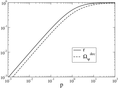
Figure 1: The dashed line shows the abundance of $\psi$ at its decay, $\Omega_{\psi}^{\rm dec}$, as a function of the initial parameter $p$. This is compared to the efficiency parameter $r$ (solid line), defined in Sec. 5.2.

Thus, the condition for $\psi$ to dominate the universe becomes $p\mathrel{\hbox to0.0pt{\lower 3.0pt\hbox{$\mathchar 536\relax$}\hss}\raise 2.0pt\hbox{$\mathchar 318\relax$}}1$.

Now we want to translate this into a condition on the decay rate and annihilation cross section of $\psi$. On using the definition of $p$, Eq. (14), we can write the condition for the domination as

$$p\simeq g^{1/4}\frac{n_{\psi}}{s}\frac{m_{\psi}}{\sqrt{m_{\rm P}\Gamma}}\mathrel{\hbox to0.0pt{\lower 3.0pt\hbox{$\mathchar 536\relax$}\hss}\raise 2.0pt\hbox{$\mathchar 318\relax$}}1,$$ (15)

where $g$ is the number of relativistic degrees of freedom and $n_{\psi}/s$ is the relic abundance of the $\psi$ particles when they freeze-out – $s$ is the entropy density. In order to derive (15) we have used $\rho\simeq\rho_{\gamma}\simeq gT^{4}$, and $s\simeq gT^{3}$.

After freeze-out and for $\Gamma\ll H$, the relic abundance $n_{\psi}/s$ is constant (we assume $g$ constant). The relic abundance can be evaluated by solving the Boltzmann equation describing the freeze out of the annihilation of $\psi$ particles and antiparticles with cross section $\sigma_{A}$, which we take to be independent of the particles energy. In this case there is an approximate solution for the abundance at freeze-out [18],

$$\frac{n_{\psi}}{s}\simeq\frac{100}{m_{\psi}m_{\rm P}g^{1/2}\langle\sigma_{A}v\rangle},$$ (16)

where $\langle\sigma_{A}v\rangle$ is the thermal average of the total cross section times the relative velocity $v$. On using this solution, Eq. (15) becomes independent of the mass $m_{\psi}$ [12],

$$p\simeq\frac{100}{g^{1/4}}\left(\frac{m_{\rm P}}{\Gamma}\right)^{1/2}\frac{m_{\rm P}^{-2}}{\langle\sigma_{A}v\rangle}\mathrel{\hbox to0.0pt{\lower 3.0pt\hbox{$\mathchar 536\relax$}\hss}\raise 2.0pt\hbox{$\mathchar 318\relax$}}1.$$ (17)

This relation holds if the $\psi$-particles are subdominant at freeze-out. The smaller the annihilation cross section is, the earlier $\psi$ freeze out before becoming non-relativistic and the larger is $\Omega^{\rm dec}_{\psi}$.

On requiring that the massive particles decay before nucleosynthesis, i.e., $\Gamma\mathrel{\hbox to0.0pt{\lower 3.0pt\hbox{$\mathchar 536\relax$}\hss}\raise 2.0pt\hbox{$\mathchar 318\relax$}}(1{\rm MeV})^{2}/m_{\rm P}$, we find that only for $\langle\sigma_{A}v\rangle\mathrel{\hbox to0.0pt{\lower 3.0pt\hbox{$\mathchar 536\relax$}\hss}\raise 2.0pt\hbox{$\mathchar 316\relax$}}10/g^{1/2}(10^{7}{\rm GeV})^{-2}$ does $\psi$ dominate the universe. Hence, the initial thermal equilibrium by annihilation of particles and antiparticles must be maintained by some gauge interaction which is weaker than those of the standard model. This excludes that $\psi$ is made of standard model particles.

5 Cosmological perturbations from the mass domination

In this section we derive the coupled perturbed equations of motion for the two fluids and the scalar field. Then we discuss their solutions, analytically and numerically. The aim is to study the mechanism of conversion of scalar field fluctuations into curvature perturbations during the mass domination.

We describe scalar perturbations in the metric with line element

$$ds^{2}=-(1+2\Phi)dt^{2}+a^{2}(1-2\Phi)\delta_{ij}dx^{i}dx^{j},$$ (18)

which follows from the absence of anisotropic stress perturbations. The quantity $\Phi$ corresponds to the Bardeen potential in longitudinal gauge.

In order to perturb the energy-momentum tensor of the three components $\psi$, $\gamma$, and $\phi$, we introduce the energy density and pressure perturbations, $\delta\rho_{X}$ and $\delta P_{X}$, and the scalar field perturbation $\delta\phi$. It is also useful to define the relative perturbation $\delta_{X}=\delta\rho_{X}/\rho_{X}$. In terms of these quantities, we perturb Eqs. (3), (4), and (7), and since we are interested in the large scale perturbations, we drop the gradient terms, that vanish in the large scale limit. This yields

$$\dot{\delta}_{\psi}-3\dot{\Phi}={{\left(\alpha\frac{\delta\phi}{\phi}\right)}^{\hbox{.}}}-\Gamma\Phi,$$ (19)

$$\dot{\delta}_{\gamma}-4\dot{\Phi}=\Gamma\frac{\rho_{\psi}}{\rho_{\gamma}}(\delta_{\psi}-\delta_{\gamma}+\Phi),$$ (20)

$$\ddot{\delta\phi}+3H\dot{\delta\phi}+\left(m_{\phi}^{2}+\frac{{{(\alpha/\phi)}^{\hbox{.}}}}{\dot{\phi}}\rho_{\psi}\right)\delta\phi=\quad$$

$$4\dot{\Phi}\dot{\phi}-2V^{\prime}\Phi-(\alpha/\phi)\rho_{\psi}(\delta_{\psi}+2\Phi).$$ (21)

The perturbed energy constraint equation reads

$$6H(\dot{\Phi}+H\Phi)=-m^{-2}_{\rm P}(\rho_{\psi}\delta_{\psi}+\rho_{\gamma}\delta_{\gamma}+\rho_{\phi}\delta_{\phi}).$$ (22)

Equation (21) can be opportunely simplified: Since the scalar field is light and subdominant we can neglect the right hand side. Assuming the strong constraint (10) we can also neglect the mass correction due to the coupling. Equation (21) then simplifies to the equation of a light test field,

$$\ddot{\delta\phi}+3H\dot{\delta\phi}+m_{\phi}^{2}\delta\phi=0,$$ (23)

that in the massive case is the same as the equation for the background field. Hence, the ratio between $\delta\phi$ and $\phi$ is constant in time,

$$\delta\phi/\phi=\delta\phi_{*}/\phi_{*}.$$ (24)

Assuming only the weaker constraint (9) implies that $\delta\phi/\phi$ may slowly vary, which makes the mechanism more difficult to study, although it maintains its qualitative features.

5.1 Analytic calculation

It is possible to analytically solve the system of equations (19), (20), and (22), in the case that the massive particles dominate completely the universe before decaying. We can hence consistently assume that we are far from the decay, $H\gg\Gamma$, so that the source terms proportional to $\Gamma$ in Eqs. (19) and (20) can be neglected for the moment. Equations (19) and (20) then simplify,

$$\dot{\delta}_{\psi}-3\dot{\Phi} = \dot{\alpha}{\delta\phi_{*}}/\phi_{*},$$ (25)

$$\dot{\delta}_{\gamma}-4\dot{\Phi} = 0,$$ (26)

where we have used Eq. (24).

We first discuss the initial conditions of these equations. They are defined in the radiation dominated era, just after the freeze-out of $\psi$. In this limit the Bardeen potential $\Phi$ is constant, and the perturbation of the radiation fluid can be found from the constraint (22), on using $\rho\simeq\rho_{\gamma}$. This yields $\delta^{(i)}_{\gamma}=-2\Phi_{*}$, where $\Phi_{*}$ is the value of $\Phi$ at the beginning of the radiation dominated era (e.g., after inflation). This initial perturbation is usually dropped and considered negligible in the treatment of models where perturbations are produced after inflation by a light field. Here however, in the spirit of [19], we retain this term since it can turn out to be larger than the curvature perturbation generated by the mass domination (see below).

The value of the initial condition $\delta_{\psi}^{(i)}$ is crucial to correctly determine the final curvature perturbation produced. Unfortunately it is not unambiguously defined. Here we set $\delta_{\psi}^{(i)}$ by assuming that radiation and $\psi$ particles were created by the same mechanism (e.g., reheating) with the same number density perturbation,

$$\delta\left(\frac{n^{(i)}_{\psi}}{n^{(i)}_{\gamma}}\right)=0\quad\Rightarrow\quad\frac{\delta n^{(i)}_{\psi}}{n^{(i)}_{\psi}}=\frac{3}{4}\delta^{(i)}_{\gamma}.$$ (27)

Thus, considering also the mass fluctuation, the relative initial density perturbation of $\psi$ reads

$$\delta^{(i)}_{\psi}=\frac{\delta m^{(i)}_{\psi}}{m^{(i)}_{\psi}}+\frac{\delta n^{(i)}_{\psi}}{n^{(i)}_{\psi}}=\alpha_{*}\frac{\delta\phi_{*}}{\phi_{*}}+\frac{3}{4}\delta^{(i)}_{\gamma}.$$ (28)

The initial conditions are thus given by

$$\Phi^{(i)}=\Phi_{*},\quad\delta\phi^{(i)}=\delta\phi_{*},\quad\dot{\delta\phi}^{(i)}=0,$$

$$\delta_{\psi}^{(i)}=\alpha_{*}\delta\phi_{*}/\phi_{*}-(3/2)\Phi_{*},\quad\delta_{\gamma}^{(i)}=-2\Phi_{*}.$$ (29)

Equations (25) and (26) can be easily solved with these initial conditions, yielding

$$\delta_{\psi} = \alpha\frac{\delta\phi_{*}}{\phi_{*}}+3\Phi-\frac{9}{2}\Phi_{*},$$ (30)

$$\delta_{\gamma} = 4\Phi-6\Phi_{*},$$ (31)

where the terms proportional to $\Phi_{*}$ are integration constants. Only the first of these equations is used in the following. At the final stage of the mass domination, when the non-relativistic particles dominate the universe, the constraint (22) yields $\delta_{\psi}=-2\Phi$. Combined with Eq. (30) it implies that the final curvature perturbation is

$$\Phi=\frac{9}{10}\Phi_{*}-\frac{1}{5}\alpha\frac{\delta\phi_{*}}{\phi_{*}}.$$ (32)

This result holds during the matter ($\psi$) dominated era, before the decay of the massive particles. It is related to the curvature perturbation in the subsequent radiation era after $\psi$ decay by the well-known relation $\Phi_{r}=(10/9)\Phi_{m}$ [1].

Equation (32) can be expressed in terms of the curvature perturbation defined on the uniform density hypersurface, $\zeta=-\Phi+{\delta\rho}/[{3(\rho+P)}]$ [20], which is known to be conserved for adiabatic perturbations. In the radiation dominated era $\zeta=-(3/2)\Phi_{r}$, which yields

$$\zeta=\zeta_{*}+\frac{1}{3}\left.\frac{\delta m_{\psi}}{m_{\psi}}\right|_{\rm dec}\quad(\Omega_{\psi}^{\rm dec}=1).$$ (33)

The coefficient $1/3$ in this equation confirms the result of [11].

5.2 Numerical results

Here we solve Eqs. (19), (20), and (22) numerically, so that we can study the case where the massive particles do not dominate the universe completely before decaying. We initially consider the particular case of $\alpha=$ constant (e.g., $m_{\psi}=\lambda\phi^{n}$). In this case the first term on the right hand side of Eq. (19) vanishes. The problem then reduces to the study of a pressureless fluid with non-vanishing initial perturbation (28) that decays into a relativistic fluid $\gamma$.

This problem has been studied in [13] in the case of the curvaton field. There, it was found that the final curvature perturbation is $\zeta=\frac{1}{3}r\delta_{\psi}$ ($\Phi_{*}=0$ was assumed), where $r$ is an efficiency parameter which can be computed as a function of $p$. We have solved Eqs. (19) and (20) numerically and the solution is

$$\zeta=\zeta_{*}+\frac{r}{3}\alpha_{*}\frac{\delta\phi_{*}}{\phi_{*}},\quad(m_{\psi}=\lambda\phi,\ \ r\simeq\Omega_{\psi}^{\rm dec}),$$ (34)

with $r\leq 1$ represented in Fig. 1. Here an initial non-vanishing perturbation $\zeta_{*}$ has also been included. Fig. 1 shows that $r\simeq\Omega_{\psi}^{\rm dec}$. As expected, the more $\psi$ dominates the universe before decaying, the more the mechanism of generation of curvature perturbations is efficient.

If $\alpha$ varies slowly during the phase of domination and decaying, we can extend the results of the numerical calculation to a general $\alpha$. We find

$$\zeta=\zeta_{*}+\frac{r}{3}\alpha_{\rm dec}\frac{\delta\phi_{*}}{\phi_{*}}=\zeta_{*}+\frac{r}{3}\left.\frac{\delta m_{\psi}}{m_{\psi}}\right|_{\rm dec}.$$ (35)

This is our main result. It generalizes the results of [11] to the case where the non-relativistic particles do not dominate the universe completely before decaying into radiation.

6 Non-Gaussianities

Here we discuss an unambiguous observational consequence of the mass domination, namely the presence of non-Gaussianities in the perturbations. The non-Gaussianities generated by the mass domination have been first computed in [11] in the case of total domination ($\Omega_{\psi}^{\rm dec}=1$) (see also [21, 22]). The possible presence of isocurvature perturbations has been studied in [12].

For convenience we define $\tilde{r}=r\alpha_{\rm dec}\simeq\Omega_{\psi}^{\rm dec}\alpha_{\rm dec}$. We also define the ratio between the perturbation generated by the mass domination and the primordial curvature perturbation $\zeta_{*}$ [see Eq. (35)],

$$R=\frac{1}{\zeta_{*}}\frac{\tilde{r}}{3}\frac{\delta\phi_{*}}{\phi_{*}}.$$ (36)

We can parameterize the level of non-Gaussianities with the non-linear parameter $f_{\rm NL}$ defined as $\zeta=\zeta_{\rm L}-({3}/{5})f_{\rm NL}\zeta_{\rm L}^{2}$ [23, 24], where $\zeta_{\rm L}$ represents the Gaussian (linear) contribution to the total curvature perturbation $\zeta$. Motivated by inflation, we assume $\zeta_{*}$ to be Gaussian.

Non-Gaussianities arise when the field perturbation $\delta\phi_{*}$ becomes larger than $\sim 10^{-4}\phi_{*}$. This happens when the efficiency is low, $\tilde{r}\ll 1$. In this case, terms quadratic in $\delta\phi_{*}/\phi_{*}$, that have been neglected in the linear calculation, become important [5, 11],

$$\zeta=\frac{\tilde{r}}{3}\left(\frac{\delta\phi_{*}}{\phi_{*}}+\frac{1}{2}\frac{\delta{\phi_{*}}^{2}}{{\phi_{*}}^{2}}\right)+\zeta_{*}.$$ (37)

This yields the non-linear parameter

$$f_{\rm NL}=-\frac{5}{2\tilde{r}}(1+R^{-1})^{-2}.$$ (38)

As expected, when $R\to 0$, $f_{\rm NL}\to 0$. If, on the contrary, $R$ is large, i.e., $\zeta$ is mainly due to the mass domination, $f_{\rm NL}=-{5}/({2\tilde{r}})$ [11]. As noticed in [5, 11] this number is in the ballpark of future experiments like Planck, that will be able to detect $f_{\rm NL}\mathrel{\hbox to0.0pt{\lower 3.0pt\hbox{$\mathchar 536\relax$}\hss}\raise 2.0pt\hbox{$\mathchar 318\relax$}}5$ at $2\sigma$-level [23]. Therefore we may have a well detectable signature of non-Gaussianities if $\tilde{r}\mathrel{\hbox to0.0pt{\lower 3.0pt\hbox{$\mathchar 536\relax$}\hss}\raise 2.0pt\hbox{$\mathchar 316\relax$}}0.5$.

Here we are also interested in the lower bound on $\tilde{r}$ from the current bound on non-Gaussianities. The WMAP limit on $f_{\rm NL}$ corresponds to $-58<f_{\rm NL}<134$ ($2\sigma$-level) [25], which translates into $\tilde{r}\mathrel{\hbox to0.0pt{\lower 3.0pt\hbox{$\mathchar 536\relax$}\hss}\raise 2.0pt\hbox{$\mathchar 318\relax$}}0.02$.

7 Liberating inflation?

As mentioned in the introduction, the main reason to use a light field other than the inflaton as a source of curvature perturbations is to liberate the inflaton from the task of generating the observed amplitude of perturbations.

In [19] (see also [26]) it was shown that, if cosmological perturbations are produced during the late decay of a light scalar field whose value during inflation is of the order of $m_{\rm P}$, then the primordial curvature perturbation already present from inflation, i.e., $\zeta_{*}$, is of the same order of magnitude as the perturbation produced by the late decay. This is true only if inflation is of slow-roll type, and fluctuations in the inflaton field are $\sim H_{*}$, i.e., of the same amplitude as the fluctuations in the light field $\phi$. It is thus interesting to compare these two contributions in the context of the mass domination.

The curvature perturbation $\zeta_{*}$ from inflation is, at first order in the slow-roll parameters, $\zeta_{*}=({1}/{\sqrt{2\epsilon}})({H_{*}}/{m_{\rm P}})$ [1], where $\epsilon\ll 1$ is the first slow-roll parameter. We can replace this expression in the definition of $R$, Eq. (36),

$$R=\tilde{r}\frac{\sqrt{2\epsilon}}{3}\frac{m_{\rm P}}{\phi_{*}}.$$ (39)

Unless $\phi_{*}$ is very small, $\phi_{*}\sim\tilde{r}\sqrt{\epsilon}m_{\rm P}$, the perturbation generated by the mass domination represents only a negligible correction to the perturbation originally present from inflation. However, we know that $\phi_{*}$ cannot be too small: Indeed, Eq. (9) implies that $\phi_{*}/m_{\rm P}>\tilde{r}^{1/2}$, which combined with Eq. (39) yields

$$R\mathrel{\hbox to0.0pt{\lower 3.0pt\hbox{$\mathchar 536\relax$}\hss}\raise 2.0pt\hbox{$\mathchar 316\relax$}}0.5\tilde{r}^{1/2}\sqrt{\epsilon}.$$ (40)

The stronger condition (10) implies an even lower value of $R$. We conclude that if inflation is of slow-roll type, the mass domination mechanism does not provide a sufficient amplitude of fluctuations to liberate inflation.

This conclusion however changes if the inflaton does not go through a standard slow-rolling phase, as proposed in [3]. If the inflaton is not light during inflation, its fluctuation is suppressed [27] and the primordial curvature perturbation originated during inflation is negligible, $\zeta_{*}\simeq 0$. Only in this case, the inhomogeneous mass domination mechanism represents a viable scenario for the generation of primordial cosmological perturbations.

8 Conclusion

We have considered the possibility that cosmological perturbations are generated by the mass domination mechanism, as proposed in [11], during a phase of domination of non-relativistic particles whose mass is fluctuating in time and space, modulated by a light scalar field. By requiring that the scalar field remains light until the massive particles decay and does not dominate the universe with a second stage of inflation, we have shown that its value must be of the order of the Planck mass. A further condition must be imposed on the annihilation cross section of the massive particles. This must be weak enough – weaker than for standard model interactions – as to let the massive particles freeze out before being completely diluted when they become non-relativistic.

We show that if these conditions are met, a curvature perturbation is produced. This is proportional to the mass fluctuation and the abundance of massive particles at their decay, as given by Eq. (35), and confirms [11], in the limit where the massive particles completely dominate the universe. Non-Gaussianities are inversely proportional to the abundance of massive particles at their decay, so that the latter can not be too small.

Perturbations produced during inflation add to those generated by the mass domination. If inflation if of slow-roll type, the former are much larger than the latter. Only for inflationary models that violate the slow-roll conditions is the mass domination a successful mechanism for generating the observed cosmological perturbations.

References

- [1] A. R. Liddle and D. H. Lyth, “Cosmological inflation and large-scale structure,” Cambridge Univ. Press, Cambridge, UK (2000).
- [2] K. Dimopoulos and D. H. Lyth, Phys. Rev. D69 123509 (2004).
- [3] N. Arkani-Hamed, S. Dimopoulos, G. Dvali and G. Gabadadze, arXiv:hep-th/0209227; G. Dvali and S. Kachru, arXiv:hep-th/0309095.
- [4] K. Enqvist and M. S. Sloth, Nucl. Phys. B 626, 395 (2002); D. H. Lyth and D. Wands, Phys. Lett. B 524, 5 (2002); T. Moroi and T. Takahashi, Phys. Lett. B 522, 215 (2001) [Erratum-ibid. B 539, 303 (2002)].
- [5] D. H. Lyth, C. Ungarelli and D. Wands, Phys. Rev. D 67, 023503 (2003).
- [6] G. Dvali, A. Gruzinov and M. Zaldarriaga, Phys. Rev. D69, 023505 (2004); L. Kofman, arXiv:astro-ph/0303614.
- [7] F. Bernardeau, L. Kofman and J. P. Uzan, Phys. Rev. D70 083004 (2004).
- [8] K. Enqvist, A. Mazumdar, and M. Postma, Phys. Rev. D67, 121303 (2003); M. Postma, JCAP 0403 006 (2004); R. Allahverdi, Phys. Rev. D70 043507 (2004); L. Ackerman, C. W. Bauer, M. L. Graesser and M. B. Wise, arXiv:astro-ph/0412007; C. W. Bauer, M. L. Graesser and M. P. Salem, arXiv:astro-ph/0502113.
- [9] A. Mazumdar and M. Postma, Phys. Lett. B 1573, 5 (2003); S. Matarrese and A. Riotto, JCAP 0308, 007 (2003).
- [10] S. Tsujikawa, Phys. Rev. D68, 083510 (2003).
- [11] G. Dvali, A. Gruzinov and M. Zaldarriaga, Phys. Rev. D69 083505 (2004).
- [12] F. Vernizzi, Phys. Rev. D69 083526 (2004).
- [13] K. A. Malik, D. Wands and C. Ungarelli, Phys. Rev. D 67, 063516 (2003).
- [14] T. Damour, G. W. Gibbons and C. Gundlach, Phys. Rev. Lett. 64, 123-126 (1990); T. Damour and K. Nordtvedt, Phys. Rev. Lett. 70, 2217 (1993); T. Damour and K. Nordtvedt, Phys. Rev. D48 3436 (1993).
- [15] G. R. Farrar and P. J. Peebles, Astrophys. J. 604 1 (2004).
- [16] G. W. Anderson and S. M. Carroll, arXiv:astro-ph/9711288; M. B. Hoffman, arXiv:astro-ph/0307350.
- [17] J. Khoury and A. Weltman, Phys. Rev. D69 044026 (2004); P. Brax, C. van de Bruck, A. C. Davis, J. Khoury and A. Weltman, Phys. Rev. D70 123518 (2004).
- [18] G. Jungman, M. Kamionkowski, K. Griest, Phys. Rep. 267, 195-373 (1996).
- [19] D. Langlois and F. Vernizzi, Phys. Rev. D70 063522 (2004).
- [20] J. M. Bardeen, Phys. Rev. D22, 1882 (1980).
- [21] M. Zaldarriaga, Phys. Rev. D69 043508 (2004).
- [22] N. Bartolo, S. Matarrese and A. Riotto, Phys. Rev. D69 043503 (2004); ibid. JCAP 0401 003 (2004).
- [23] E. Komatsu and D. N. Spergel, Phys. Rev. D63, 063002 (2001).
- [24] L. Verde, L. Wang, A. F. Heavens, and M. Kamionkowski, MNRAS 313, 141 (2000).
- [25] E. Komatsu et al., Astrophys. J. Suppl. 148 119 (2003).
- [26] G. Lazarides, R. R. de Austri and R. Trotta, Phys. Rev. D70 123527 (2004); T. Moroi, T. Takahashi and Y. Toyoda, arXiv:hep-ph/0501007.
- [27] D. Langlois and F. Vernizzi, JCAP 0501 002 (2005).