Non -Thermal Emission from AGN Coronae

Accretion disk coronae are believed to account for X-ray emission in Active Galactic Nuclei (AGNs). In this paper the observed emission is assumed to be due to a population of relativistic, non-thermal electrons (e.g. produced in a flare) injected at the top of an accretion disk magnetic loop. While electrons stream along magnetic field lines their energy distribution evolves in time essentially because of inverse Compton and synchrotron losses. The corresponding time dependent emission due, in the X-ray energy range, to the inverse Compton mechanism, has been computed. Since the typical decay time of a flare is shorter than the integration time for data acquisition in the X-ray domain, the resulting spectrum is derived as the temporal mean of the real, time-dependent, emission, as originated by a series of consecutive and identical flares. The model outcome is compared to both the broad band BeppoSAX X-ray data of the bright Seyfert 1 NGC 5548, and to a few general X-ray spectral properties of Seyfert 1s as a class. The good agreement between model and observations suggests that the presently proposed non-thermal, non-stationary model could be a plausible explanation of AGN X-ray emission, as an alternative to thermal coronae models.

1 Introduction

In these last years the idea of a hot corona lying above the AGN accretion disk has been developed in order to account for substantial emission in the X-ray energy range. Indeed, the original suggestion of this scenario dates back to 1977 (Liang & Price liang77 (1977)), referring to the X-ray binaries’ context, and to 1979 (Liang liang79 (1979)), more specifically regarding AGN X-ray emission. The hot corona can, in fact, Comptonize the soft photons emitted by the “cool” accretion disk, thus producing high energy radiation. Several scenarios have been developed for AGN coronae, both analytically and numerically (Poutanen & Svensson pout (1996); Dove et al. dove (1997); Di Matteo dima98 (1998); Merloni & Fabian merlo (2001); Miller & Stone misto00 (2000)). Haardt & Maraschi (hm91 (1991), hm93 (1993)) analyzed in detail and developed the idea of a radiative coupling between the two phases of the system (disk+corona); subsequently, in order to better match the observations, Haardt et al. (hmg94 (1994)) have developed a more detailed model of a non-uniform, blob-like corona. From the physical point of view, in the above papers the hot corona is assumed as the a region where at least part of the accretion gravitational energy is released. The existence of an optically thin coronal structure, sandwiching the disk and characterized by a strong magnetic coupling with the optically thick disk, was firstly suggested by Galeev et al. (ga79 (1979)). The idea is that the accretion disk differential rotation, together with the natural presence of a magnetic field, could reproduce a situation analogous to that present in the atmospheres of convective stars. As Heyvaerts & Priest (hp89 (1989)) have shown, loops and arcades can form also in AGN accretion disks; these structures, connecting remote points of the disk itself, can convert disk kinetic energy into magnetic energy and subsequently dissipate it by emitting the observed spectrum. Magnetic reconnection is invoked as the physical process responsible for this last conversion, even though all the details of the process itself are not yet understood.

An issue that has not yet been clarified is whether the analogy between stellar and AGN coronae is limited to the above described features or whether it is more comprehensive. Once a physical description is chosen in which the magnetic field is responsible for transferring accretion energy from the disk to the AGN corona, we can ask ourselves whether the magnetic field can act in a different way and produce a different environment with respect to the stellar case. It seems reasonable that if the global picture of a stellar corona is applicable in the AGN context, the same should be true for the relevant physical processes as well. The analysis of solar flares has shown (see Masuda et al. (masu94 (1994)) for a short summary) that accelerated particles are responsible for the hard ($>10$ keV) X-ray emission via the bremsstrahlung interaction with thermal matter. Moreover, even in the absence of conspicuous flares, X-ray brightenings and type III radio bursts show the presence of non-thermal electron beams in the solar corona (Klein et al. kl97 (1997)). Hence, the existence of impulsive injection of non-thermal particles seems to be a common ingredient in the physics of stellar coronae. The question we are interested in is whether, in the specific AGN context, an impulsive, non-thermal electron distribution can be responsible for the emission of the observed X-ray radiation or, on the contrary, a stationary and thermal electron population at high temperature (like the one adopted in the model proposed by Haardt & Maraschi (hm91 (1991),hm93 (1993)), and Haardt et al. (hmg94 (1994))) Comptonizing the soft disk photons is the only possible explanation of the observed high energy emission.

Stationary non-thermal models have been developed starting from the 1980s in order to explain AGN X-ray emission (for a review see Svensson sv94 (1994) and Ghisellini ghise94 (1994)); however, these models, at least in their “standard” versions (Svensson sv94 (1994); Svensson sv96 (1996)), showed some problems as for the reproduction of high energy observations of Seyfert spectra by OSSE, in particular referring to the indications of high energy cutoffs in the spectra, and to the lack of detections at $\sim$ 0.75-3 MeV by COMPTEL (Svensson sv96 (1996); Haardt haardt97 (1997)). In our framework, impulsive injection of the relativistic electron population is determinant for what regards the specific characteristics of the non-thermal model we are proposing, because it is exactly this feature that makes the model intrinsically non-stationary. This peculiar property of our scenario distinguishes it from previous “standard” non-thermal models and will be explained and discussed in the following Sections.

Therefore, starting from the knowledge that we have of solar/stellar coronae mechanisms and trying to extend it to the AGN coronae scenario, we shall investigate the time evolution (see Sect. 2) and the emission (see Sect. 3) of an ensemble of accelerated non-thermal electrons injected in a magnetic loop. How these accelerated particles are produced is not relevant to the following analysis and, on the other hand, it is still matter of debate even in the solar corona, although it seems to be plausibly related to magnetic activity processes (such as reconnection).
In Sect. 4 we describe and discuss the application of the model that we have devised to the Seyfert 1 galaxy NGC 5548; in Sect. 5 the results of this analysis are compared to BeppoSAX observations. Sect. 6 is devoted to the discussion of the descriptive capability of the model regarding to general trends and properties identified for Seyfert 1 X-ray spectra, in order to test our model’s relevance with respect to this type of source. Finally, Section 7 includes both an analysis of our model as compared with previous models in literature, and the conclusions we draw from the present work.

2 Behavior of accelerated electrons

When a certain amount of accelerated electrons is injected around the top of a magnetic loop, part of them is trapped within the curved magnetic field lines, while part of them precipitates in the denser plasma, where the loop bases are anchored. The electrons which are magnetically reflected inside the loop loose their energy by colliding with the thermal plasma present in the loop and by emitting synchrotron, inverse Compton (IC) and bremsstrahlung (BR) radiation. How long it takes to thermalize these electrons and how the electron energy distribution changes in time is analyzed hereafter. The group of precipitating electrons interacts with the denser plasma (of the disk or of the photosphere) and stops after a rapid bremsstrahlung emission. This emission is what we identify with the hard X-ray ($>10$ keV) emission in solar flares.

The relative importance of the trapped and of the precipitated electrons depends on the specific physical configuration and on the density gradient of thermal matter in the loop.

An estimate of the typical loop extension in the AGN accretion disk corona context can be obtained for instance following Di Matteo (dima98 (1998)): extending the results of solar atmosphere magnetic buoyancy simulations (Shibata et al. shibata89 (1989)), this author gives an estimate of the loop top height ($H_{\rm{flare}}$), which reads $H_{\rm{flare}}\sim 8H_{\rm{disk}}$, where $H_{\rm{disk}}$ is the pressure scale height of the accretion disk. Furthermore, if, still following Di Matteo (dima98 (1998)), we remind that, for a standard Shakura & Sunyaev (ss73 (1973)) disk, it is $H_{\rm{disk}}/R\la 0.1$ (where $R$ is the radial distance from the central black hole on the disk midplane), we can relate $H_{\rm{flare}}$ to the Schwarzschild radius, $R_{\rm S}\equiv 2GM_{\rm BH}/c^{2}$; in fact, for the accreting disk central regions we can assume a representative radial distance from the black hole $R\sim 10R_{\rm S}$, and this leads to the following approximate relation $H_{\rm{flare}}\la 8R_{\rm S}$ and, finally, to the estimate $H_{\rm{flare}}\la 2.36\times 10^{13}(M_{\rm BH}/10^{7}M_{\odot})$ cm. Other approximate estimates of coronal region extension can be found in the work of Miller & Stone (misto00 (2000)), whose MHD numerical simulations of a coronal structure formation above a weakly magnetized accretion disk indicate that, in the specific conditions of the simulation at least, most of the buoyantly rising magnetic energy is dissipated between 3 and 5 disk scale heights (i.e., what we have called $H_{\rm{disk}}$) above the disk itself, and in the work of Liu, Mineshige & Shibata (liu02 (2002)), who cite a representative size value $\sim 10R_{\rm S}$ cm. All the above cited estimates are, in conclusion, in substantial agreement with an evaluation of $H_{\rm{flare}}$ ranging from $\sim 3R_{\rm S}$ to $\sim 10R_{\rm S}$.

This allows us to finally estimate the typical electron dynamical time in the loop, that can be defined as $t_{\rm dyn}=H_{\rm{flare}}/c$ and represents the time it takes for the electrons to reach the disk; we also define a characteristic radiation time, $t_{\rm emis}$, as the typical time it takes for the radiation emitted around 10 keV (the energy range we are mainly interested in) to decrease by a factor of twenty in luminosity. When $t_{\rm emis}<t_{\rm dyn}$ the electron distribution evolves on short time scales with respect to the dynamical timescale and it is depleted before reaching the the impact region; in this limit the energy lost as impulsive bremsstrahlung emission can be disregarded. This appears to be the case in the AGN coronal environment, as it will be verified in Sect. 4.

2.1 Electron energy loss rates

Given an electron energy distribution

$$n(\gamma_{\rm o},t=0)=n_{\rm o}(\gamma_{\rm o}-1)^{-s}\leavevmode\nobreak\ \leavevmode\nobreak\ \leavevmode\nobreak\ {\rm el./cm^{3}/}d\gamma,$$ (1)

where $\gamma_{\rm o}\equiv\gamma(t=0)$, in the energy range (in units of $m_{\rm e}c^{2}$, where $m_{\rm e}$ is the electron rest mass)

$$1\leq\gamma_{\rm o1}\leq\gamma_{\rm o}\leq\gamma_{\rm o2},$$

this distribution evolves subject to the system energy losses. The relevant energy loss rates for the present problem are in principle the following (see, e.g., Ginzburg gin (1969); Lang lang (1980); Blumenthal & Gould blum (1970) ):

$\bullet$ collision losses in the relativistic limit :

$${d\gamma\over dt}=-1.5\times 10^{-14}n_{\rm th}[73.4+\ln(\gamma/n_{\rm th})]\leavevmode\nobreak\ {\rm s}^{-1},$$

where $n_{\rm th}$ is the thermal density inside the loop and it is expressed in cm^-3; this expression can be further approximated as follows

$${d\gamma\over dt}\simeq-1.5\times 10^{-14}n_{\rm th}[74.4-\ln(n_{\rm th})]\leavevmode\nobreak\ {\rm s}^{-1}$$

$$\leavevmode\nobreak\ \leavevmode\nobreak\ \leavevmode\nobreak\ \leavevmode\nobreak\ \leavevmode\nobreak\ \leavevmode\nobreak\ \leavevmode\nobreak\ \leavevmode\nobreak\ \leavevmode\nobreak\ \leavevmode\nobreak\ \leavevmode\nobreak\ \leavevmode\nobreak\ \leavevmode\nobreak\ \leavevmode\nobreak\ \leavevmode\nobreak\ \leavevmode\nobreak\ \leavevmode\nobreak\ \leavevmode\nobreak\ \leavevmode\nobreak\ \leavevmode\nobreak\ \leavevmode\nobreak\ \leavevmode\nobreak\ \leavevmode\nobreak\ \equiv A_{0}(n_{\rm th})\leavevmode\nobreak\ \leavevmode\nobreak\ \leavevmode\nobreak\ {\rm s}^{-1},$$ (2)

since $\ln(\gamma)$ is a small, slowly varying term in the limit where collision losses are important (see later, eq. (6));

$\bullet$ bremsstrahlung losses:

$${d\gamma\over dt}=-1.4\times 10^{-16}n_{th}[ln(\gamma)+0.36]\gamma\leavevmode\nobreak\ \leavevmode\nobreak\ {\rm s}^{-1}$$

$$\leavevmode\nobreak\ \leavevmode\nobreak\ \leavevmode\nobreak\ \leavevmode\nobreak\ \leavevmode\nobreak\ \leavevmode\nobreak\ \leavevmode\nobreak\ \leavevmode\nobreak\ \leavevmode\nobreak\ \leavevmode\nobreak\ \leavevmode\nobreak\ \leavevmode\nobreak\ \leavevmode\nobreak\ \leavevmode\nobreak\ \leavevmode\nobreak\ \leavevmode\nobreak\ \leavevmode\nobreak\ \leavevmode\nobreak\ \leavevmode\nobreak\ \leavevmode\nobreak\ \leavevmode\nobreak\ \leavevmode\nobreak\ \leavevmode\nobreak\ \equiv A_{1}(n_{\rm th},\gamma)\gamma\leavevmode\nobreak\ \leavevmode\nobreak\ {\rm s}^{-1}$$ (3)

$\bullet$ inverse Compton and synchrotron losses:

$${d\gamma\over dt}=-3.2\times 10^{-8}(U+{B^{2}\over 8\pi})\gamma^{2}\equiv A_{2}(U,B)\gamma^{2}\leavevmode\nobreak\ \leavevmode\nobreak\ {\rm s}^{-1}$$ (4)

where $B$ is the magnetic field (in gauss) and $U$ is the energy density (erg/cm³) of soft photon radiation field present in the loop structure. If  $L_{\rm soft}(\epsilon$) (erg s^-1keV^-1) is the seed (IR-UV) photon source spectral luminosity coming from the AGN disk and $L_{\rm local}(\epsilon$) (erg s^-1keV^-1) is the radiation field luminosity (see eq. (10) in Sect. 3 for its explicit definition) emitted by the electrons of the relativistic distribution through synchrotron mechanism in the local magnetic field, then $U$ (erg cm^-3) can be derived as

$$U={1\over 4\pi c}F_{\rm geom}(R_{\rm UV-X})\int^{\epsilon_{\rm Max}}_{\epsilon_{\rm min}}L_{\rm soft}(\epsilon)\leavevmode\nobreak\ d\epsilon\leavevmode\nobreak\ \leavevmode\nobreak\ +$$

$$\leavevmode\nobreak\ \leavevmode\nobreak\ \leavevmode\nobreak\ \leavevmode\nobreak\ \leavevmode\nobreak\ \leavevmode\nobreak\ \leavevmode\nobreak\ \leavevmode\nobreak\ \leavevmode\nobreak\ \leavevmode\nobreak\ \leavevmode\nobreak\ \leavevmode\nobreak\ \leavevmode\nobreak\ \leavevmode\nobreak\ \leavevmode\nobreak\ \leavevmode\nobreak\ \leavevmode\nobreak\ \leavevmode\nobreak\ \leavevmode\nobreak\ \leavevmode\nobreak\ \leavevmode\nobreak\ \leavevmode\nobreak\ \leavevmode\nobreak\ \leavevmode\nobreak\ \leavevmode\nobreak\ \leavevmode\nobreak\ \leavevmode\nobreak\ \leavevmode\nobreak\ \leavevmode\nobreak\ \leavevmode\nobreak\ \leavevmode\nobreak\ {3\over 4\pi cR^{2}_{\rm em}}\int^{\epsilon_{\rm Max}}_{\epsilon_{\rm min}}L_{\rm local}(\epsilon)\leavevmode\nobreak\ d\epsilon\leavevmode\nobreak\ \leavevmode\nobreak\ \leavevmode\nobreak\ \leavevmode\nobreak\ \leavevmode\nobreak\$$ (5)

where $\epsilon$ is the photon energy, that we express in keV, in the range $\epsilon_{\rm min}\leq\epsilon\leq\epsilon_{\rm Max}$. In this expression we take $\epsilon_{\rm min}=10^{-5}$ keV and $\epsilon_{\rm Max}=0.1$ keV, $R_{\rm UV-X}$ is the mean distance between the source of soft photons and the X-ray emitting loop structure and $R_{\rm em}$ is the characteristic length scale of the emitting region. The quantity $F_{\rm geom}(R_{\rm UV-X})$ is sort of a geometric factor, accounting for the fact that soft radiation from the disk reaches the coronal region from different different positions in the disk and therefore is differently “diluted”. We adopt a simplified treatment of this effect, following Ghisellini et al. (ghise04 (2004)) (see their eq. (14)), so that it can be represented by the quantity $F_{\rm geom}(R_{\rm UV-X})$, which depends basically only on a length scale representative of the vertical distance of the X-ray emitting structure from the disk itself, namely $R_{\rm UV-X}$.

All the above energy losses make the electron distribution change its energy dependence. However, depending on the physical conditions of the plasma, their relative importance can be rather different, and in the following we discuss this issue referring to the coronal environment of our model scenario.

First, bremsstrahlung losses do not seem to play an important role in the electron distribution evolution for the typical range of $n_{\rm th}$ that we can estimate for our problem: they are negligible with respect to collision losses for $\gamma<200$ and with respect to Inverse Compton and synchrotron losses for $\gamma>200$, if $B>50$ gauss and $n_{\rm th}<10^{11}$ cm^-3. In the context of AGN coronae these limitations on the values of magnetic field and thermal density seem to be reasonably met and they do not pose very stringent conditions. In particular, this is true in the framework of the model we are defining for coronal emission, whose origin we imagine to be non-thermal. In fact, we have to require that a thermal component in the coronal loops has negligible effects on the resulting X-ray spectrum. In other words, we want to disregard any possible thermal Comptonization or recoil effects on the spectrum itself. This implies a tighter upper limit for the density ($n_{\rm th}$) of the thermal component of the coronal loops (see Sect. 4.3 for a more detailed discussion and estimate for the case of NGC 5548). In the light of the above considerations, we can therefore safely conclude that, in the context of AGN coronae and in particular in our model scenario, the range of plausible physical conditions is such that bremsstrahlung losses are basically ineffective with respect to those due to IC and synchrotron processes.

Secondly, for what regards collision losses, we can note that at low energies these will make the distribution flatter, while inverse Compton and synchrotron losses will steepen it at high energies. A critical value for the electron energy can be easily derived comparing eq.s (2) and (4), when $A_{0}\geq A_{2}$:

$$\leavevmode\nobreak\ \leavevmode\nobreak\ \leavevmode\nobreak\ \leavevmode\nobreak\ \leavevmode\nobreak\ \leavevmode\nobreak\ \gamma_{\rm lim}\equiv\sqrt{{A_{0}\over A_{2}}}\simeq 5\times 10^{-3}\sqrt{{n_{\rm th}\over U+B^{2}/8\pi}}.$$ (6)

Inverse Compton and synchrotron losses are the most efficient for $\gamma>\gamma_{\rm lim}$, while for $\gamma<\gamma_{\rm lim}$ collision losses are the most important ones. Adopting a representative value for the coronal structure scale length $\sim 5R_{\rm S}$ (see Sect. 2), a rough estimate of the soft radiation energy density as $U\sim 0.01L_{Edd}/4\pi c(5R_{\rm S})^{2}$ gives $\gamma_{\rm lim}\sim 4$ for $M_{\rm BH}=10^{7}M_{\odot}$ and for a reasonable (see Section 4.3) upper limit $n_{\rm th}\sim 10^{11}$ cm^-3 for the thermal density. Furthermore, from eq. (6) it is clear that, when $A_{0}\leq A_{2}$, IC and synchrotron losses will be dominant in any case, i.e. for any meaningful value of $\gamma$. With the same order of magnitude evaluation of $U$ that we have used above, we can define an estimate of the upper limit of the thermal density to maintain the condition $A_{0}\leq A_{2}$ fulfilled, so that collision losses are effectively “negligible” with respect to IC and synchrotron losses in the electron distribution evolution for any possible physical value of $\gamma$. It turns out that, for this to occur, $n_{\rm th}<6.4\times 10^{10}$ cm^-3. Since for our model consistency (see below in the present Section and in Section 4.3 for more details) we have to require a much lower thermal density in the coronal loops, the discussion above clearly shows that in our context collisional losses can be disregarded as well.

2.2 The evolution of the electron distribution: an analytic solution

Melrose & Brown (melro76 (1976)) derived a formal method for the solution of the general equation for the evolution of a distribution function $n(\gamma,t)$ for particles in energy phase space. In the limit of negligibility of precipitating electrons (which applies to our problem as discussed in Sect. 2) this formal solution gets simplified. Taking also into account the further simplification due to the fact that bremsstrahlung and collisional losses are negligible, the remaining relevant loss rates can be expressed as proportional to a power of the electron energy $\gamma$ with a coefficient $A_{2}$ that does not depend on $\gamma$ itself, but may depend on time through the locally produced (synchrotron) luminosity, $L_{\rm local}$. This condition proves quite useful, since it makes it possible to derive, following Melrose & Brown (melro76 (1976)) formal procedure, an analytical solution for the time evolution of the initial electron energy distribution $n(\gamma_{\rm o},0)$.

The resulting time dependent electron distribution after a time $t$ can be expressed as :

$$n(\gamma,t)\leavevmode\nobreak\ \leavevmode\nobreak\ \leavevmode\nobreak\ =\leavevmode\nobreak\ \leavevmode\nobreak\ \leavevmode\nobreak\ \leavevmode\nobreak\ n_{\rm o}{1\over[1+\gamma\theta]^{2}}\left[{\gamma\over 1+\gamma\theta}-1\right]^{-s}$$ (7)

with

$$\theta=\int^{t}_{0}A_{2}(t^{\prime})dt^{\prime}.$$

The range of $\gamma$ over which the distribution extends is also evolving in time and it becomes

$$\gamma_{1}(t)\leq\gamma(t)\leq\gamma_{2}(t)$$

where

$$\gamma_{1}(t)={\gamma_{\rm o1}\over 1-\gamma_{\rm o1}\theta}$$

$$\gamma_{2}(t)={\gamma_{\rm o2}\over 1-\gamma_{\rm o2}\theta}.$$

3 The overall emission

From the above expressions for the time dependent electron distribution, inverse Compton, synchrotron and bremsstrahlung emission can be computed. Obviously the spectral luminosity due to those radiation processes evolves in time as well, owing to the time evolution of the electron distribution. As a matter of fact, in our context, the IC component is the sole significant contribution to the resulting X-ray emission in our model. Indeed, relativistic bremsstrahlung emission is not explicitly described in this Section, since it turns out to be negligible in the present scenario, as we briefly discuss in the following.

In fact, we have already shown, at the end of Sect. 2.1, that the effects of the bremsstrahlung energy loss rate on the global evolution of the relativistic electron energy spectrum are unimportant with respect to those of the other loss mechanisms at work, for whatever value of the electron energy $\gamma$, under the physical conditions expected for an AGN coronal structure like the one we want to model. This clearly implies that the corresponding bremsstrahlung emission has to be negligible as well when compared to the IC component and this is indeed what we have verified from our spectral luminosity computations. This is important to stress, since the resulting relativistic bremsstrahlung would peak at energies higher than those in the typical range of the first scattering IC component, so that, in principle, it could also happen that, although small, in the very high energy range the bremsstrahlung relative contribution to the total emission could be significant.

The effects of the synchrotron emission of relativistic electrons in the ambient magnetic field have been explicitly taken into account, as far as the electron energy losses (and, as a consequence, the relativistic electron population evolution) are concerned (see eq. (4)) and for their contribution to the seed photon spectral luminosity that is to be reprocessed through inverse Compton mechanism. Synchrotron emission does not show up directly in the resulting spectrum since, for the whole of the ranges of physical parameters that we have selected as appropriate for the present context and explored by computing the resulting spectra, it turns out that
a) due to the typical range of energies of the injected relativistic electron distribution ($\gamma_{\rm Max}\sim 10^{3}$), the synchrotron component covers a range of energies which does not belong to the X-ray domain, and, for reasonable values of the magnetic field, peaks at energies well below the optical and, moreover,
b) its emission level turns out to be below that of the observed IR-opt.-UV spectrum as reported in literature (see next Section).

However, due to the fact that synchrotron radiation is produced in the same place, i.e. a coronal loop where inverse Compton reprocessing occurs, the geometrical factor to be accounted for in the computation of its energy density makes its contribution non negligible as far as the seed photon energy density is concerned. This contribution is taken explicitly into account by the term $L_{\rm local}$ in eq. (5) and in the following eq. (8), which defines the resulting inverse Compton spectral luminosity as a function of time.

Defining $E$ (in keV) as the emitted photon energy and remembering that $\epsilon$ is the incident soft photon energy, the inverse Compton spectral luminosity, in erg s^-1 keV^-1, at a given time $t$ reads

$$\leavevmode\nobreak\ \leavevmode\nobreak\ \leavevmode\nobreak\ \leavevmode\nobreak\ \leavevmode\nobreak\ L_{\rm IC}(E,t)=7.5\times 10^{-15}{E\leavevmode\nobreak\ V_{\rm loops}\over 4\pi c}\times$$ (8)

$$\int^{\epsilon_{\rm Max}}_{\epsilon_{\rm min}}\int^{\gamma_{2}}_{\gamma_{1}}g(\gamma,\epsilon,t)\left[F_{\rm geom}{L_{\rm soft}(\epsilon)\over\epsilon^{2}}+{1\over R^{2}_{\rm em}}{L_{\rm local}(\epsilon,t)\over\epsilon^{2}}\right]\leavevmode\nobreak\ d\gamma d\epsilon,$$

where

$$g(\gamma,\epsilon,t)=\cases{{2\leavevmode\nobreak\ n(\gamma,t)\over 3\gamma^{2}}\left(1-{E\over 4\gamma^{2}\epsilon}\right)\leavevmode\nobreak\ \leavevmode\nobreak\ \leavevmode\nobreak\ \leavevmode\nobreak\ \leavevmode\nobreak\ \leavevmode\nobreak\ \leavevmode\nobreak\ \leavevmode\nobreak\ {\rm for}\leavevmode\nobreak\ \leavevmode\nobreak\ \leavevmode\nobreak\ {E\over 4\gamma^{2}\epsilon}<1\cr 0\leavevmode\nobreak\ \leavevmode\nobreak\ \leavevmode\nobreak\ \leavevmode\nobreak\ \leavevmode\nobreak\ \leavevmode\nobreak\ \leavevmode\nobreak\ \leavevmode\nobreak\ \leavevmode\nobreak\ \leavevmode\nobreak\ \leavevmode\nobreak\ \leavevmode\nobreak\ \leavevmode\nobreak\ \leavevmode\nobreak\ \leavevmode\nobreak\ \leavevmode\nobreak\ \leavevmode\nobreak\ \leavevmode\nobreak\ \leavevmode\nobreak\ \leavevmode\nobreak\ \leavevmode\nobreak\ \leavevmode\nobreak\ \leavevmode\nobreak\ \leavevmode\nobreak\ {\rm for}\leavevmode\nobreak\ \leavevmode\nobreak\ \leavevmode\nobreak\ \leavevmode\nobreak\ \leavevmode\nobreak\ \leavevmode\nobreak\ {E\over 4\gamma^{2}\epsilon}\geq 1.},$$

In the above expression, $V_{\rm loops}$ is the total volume of the part of the corona where flares take place (contributing to the emission we observe) and $L_{\rm soft}(\epsilon)$ is the illuminating IR-UV spectral luminosity from the accretion disk defined over the energy interval $[\epsilon_{\rm min},\epsilon_{\rm Max}]$ (see Sect. 2.1). We assume this soft spectrum as known, and we model it as a parameterized power-law with a high energy cut-off, as it is explicitly specified below:

$$L_{\rm soft}(\epsilon)=H_{0}\epsilon^{1-\rm UV2}e^{-\epsilon/E_{\rm cut}}\leavevmode\nobreak\ \leavevmode\nobreak\ \leavevmode\nobreak\ \leavevmode\nobreak\ \leavevmode\nobreak\ \leavevmode\nobreak\ \leavevmode\nobreak\ \leavevmode\nobreak\ \epsilon_{\rm min}<\epsilon.$$ (9)

In this expression UV2 is the photon index of the spectral distribution, $E_{\rm cut}$ is the cut-off energy (in keV), and $L_{\rm soft}$ is expressed in erg s^-1 keV^-1. Therefore, for each AGN source we intend to study, first we shall have to appropriately choose the parameters of our representation of $L_{\rm soft}(\epsilon)$, so as to fit the observed IR-UV spectrum, as described in literature.

The other term present in eq.(8) , $L_{\rm local}$, takes into account any production of soft photons by the relativistic electron distribution, namely synchrotron emission in the loop magnetic field. As outlined above, for our parameter ranges, synchrotron emission is too weak to be relevant in the observed spectrum, but its contribution as seed radiation for the IC reprocessing is non negligible. The synchrotron spectral luminosity of each single active loop is given by:

$$L_{\rm local}(\epsilon,t)=2.8\times 10^{-5}{V_{\rm loops}\over q}\leavevmode\nobreak\ B\leavevmode\nobreak\ \times\leavevmode\nobreak\ \leavevmode\nobreak\ \leavevmode\nobreak\ \leavevmode\nobreak\ \leavevmode\nobreak\ \leavevmode\nobreak\ \leavevmode\nobreak\ \leavevmode\nobreak\ \leavevmode\nobreak\ \leavevmode\nobreak\ \leavevmode\nobreak\ \leavevmode\nobreak\ \leavevmode\nobreak\ \leavevmode\nobreak\ \leavevmode\nobreak\ \leavevmode\nobreak\ \leavevmode\nobreak\ \leavevmode\nobreak\ \leavevmode\nobreak\ \leavevmode\nobreak\ \leavevmode\nobreak\ \leavevmode\nobreak\ \leavevmode\nobreak\ \leavevmode\nobreak\ \leavevmode\nobreak\ \leavevmode\nobreak\ \leavevmode\nobreak\$$ (10)

$$\leavevmode\nobreak\ \leavevmode\nobreak\ \leavevmode\nobreak\ \leavevmode\nobreak\ \leavevmode\nobreak\ \leavevmode\nobreak\ \leavevmode\nobreak\ \leavevmode\nobreak\ \leavevmode\nobreak\ \int_{\gamma_{1}}^{\gamma_{2}}d\gamma\leavevmode\nobreak\ n(\gamma,t){\epsilon\over\epsilon_{\rm c}}\int^{\infty}_{\epsilon/\epsilon_{\rm c}}K_{5/3}(\xi)d\xi\leavevmode\nobreak\ \leavevmode\nobreak\ \leavevmode\nobreak\ \leavevmode\nobreak\ \leavevmode\nobreak\ \leavevmode\nobreak\ \leavevmode\nobreak\ \leavevmode\nobreak\ {\rm erg\leavevmode\nobreak\ s}^{-1}\leavevmode\nobreak\ {\rm keV}^{-1},$$

where

$$\epsilon_{\rm c}=1.7\times 10^{-11}\gamma^{2}B\leavevmode\nobreak\ \leavevmode\nobreak\ \leavevmode\nobreak\ \leavevmode\nobreak\ \leavevmode\nobreak\ \leavevmode\nobreak\ \leavevmode\nobreak\ \leavevmode\nobreak\ \leavevmode\nobreak\ {\rm keV,}$$ (11)

$q$ is the number of active loops in the coronal structure (assumed constant in time) and $K_{5/3}$ is the modified Bessel function of order 5/3.

Expression (8) for the resulting IC spectral luminosity takes into account only the first inverse Compton scattering of the soft photons illuminating the loop, in the hypothesis that the second and the higher order ones have negligible effects on the resulting high energy spectrum in our context. The validity of this approximation will be discussed and verified in Sect. 5.

It is also important to stress that, even if this model does not belong to the “family” of thermal models, it shares with them the existence of a feedback between the flaring corona and the cold underneath disk. In fact, we assume that roughly one half of the inverse Compton emitted radiation is directed inwards, to the disk surface; this approximate fraction of the X-ray radiation will therefore be somehow reprocessed by the disk material (absorbed or “reflected”), thus implying some dependence of the disk physical conditions on the coronal emission and possibly some sort of relation between the high energy coronal emission itself and the soft disk emission. The expected complex interplay between disk and corona has been widely discussed by Haardt et al. (hmg94 (1994)). However, it is important to stress that, in accordance with Uttley et al. (uttley (2003)) conclusions, in this work we do not demand that soft radiation from the disk is only due to reprocessing of the X-ray coronal emission.

4 Application of our model to AGN X-ray sources: the example of NGC 5548

The choice of adequate observational data for testing our model is based on several criteria. Seyfert 1 galaxies (Sy 1) are excellent candidates because a substantial amount of their observed X-ray emission is believed to originate directly from the inner central regions of the accretion disk (with some reprocessing in the form of reflection and absorption). The contribution from the jet to the observed flux is believed to be negligible in this type of AGN.

To exemplify the applicability of our model and to fully illustrate our procedure in its details, we have to choose a particular source and test the model itself against the source’s observed X-ray spectrum. This is the subject of the present Section. However, the plausibility and validity of the emission model we present must be evaluated on the basis of a more general comparison with the observed properties of X-ray spectra of Seyfert 1 active nuclei. This comparison is postponed to Section 6, in which the descriptive capabilities of our model will be analyzed in order to account for a few general observed trends and properties of Seyfert 1 X-ray spectra.

For the present purposes of quantitative and detailed comparison between theory and observations, it is important to choose a bright source for which broad-band X-ray spectra are available as well as good optical/UV data. For the X-ray data the choice of BeppoSAX is obvious, because of its unparalleled broad band and sensitivity (Boella et al. 1997a ). Ideally, the optical/UV and X-ray data should be simultaneous with the X-ray data, however such data sets are extremely rare.

NGC 5548 is a well-known and nearby (z=0.017) Seyfert 1.5 galaxy, bright in the X-ray domain. It was observed several times by BeppoSAX (see Nicastro et al. nica (2000); Petrucci et al. petru (2000); Pounds et al. pounds (2003)) and a vast amount of optical and UV observations are available for it. It is among the 8 brightest type 1 Seyfert galaxies observed by BeppoSAX ($F_{2-10\leavevmode\nobreak\ {\rm keV}}\geq 4\times 10^{-11}$ erg cm^-2 s^-1).

BeppoSAX observed NGC 5548 at 3 different epochs: August 1997, December 1999 and July 2001. The source was at it brightest during the 1999 and 2001 observations. The July 2001 data set was selected for our study because the exposure at low energies (LECS instrument) is better than in 1999. We do not have simultaneous multi-wavelength data for this source (extending from the IR to the X-ray range) and, as a consequence, we rely on literature knowledge of the IR-UV spectrum in what follows.

4.1 The adopted soft photon spectrum

The parameters describing its IR to UV spectral luminosity in the simplified representation that we have introduced for this quantity in the previous section (see eq. (9)) have been selected by analyzing the results described in the literature as follows. At energies higher than $\epsilon_{\rm min}=10^{-2}$ eV (124 $\mu$) we assume UV2 $=1.3$ and a normalization luminosity, $L_{\rm soft}(2.25\leavevmode\nobreak\$eV$)=2.8\times 10^{46}$ erg s^-1 keV^-1, derived from Ward et al. (ward (1987)). Since the source is highly variable this value for the luminosity seems a good compromise between the higher value quoted by Malkan & Sargent (malkan (1982)), $L_{\rm soft}(2.25$ eV$)=3.6\times 10^{46}$ erg s^-1 keV^-1, and the luminosity range reported by Wamsteker et al. (wamst (1990)), $L_{\rm soft}(2.25$ eV$)=1.3\div 2.9\times 10^{46}$ erg s^-1 keV^-1. The value H${}_{0}=50\;\;{\rm km\;s}^{-1}{\rm Mpc}^{-1}$ has been assumed to derive the above luminosities. Note that between $\epsilon_{\rm min}$ and $\epsilon_{1}=1.8$ eV (0.7 $\mu$) the observed spectrum, like the one shown in Fig. 1, can be represented by a power-law with photon index UV1 $=2$ (Carleton et al. carle (1987)).

An exponential cut-off at $E_{\rm cut}=0.015$ keV, modifies the slope of the UV spectrum at high energies. The value has been chosen so that the energy spectrum decreases for $\lambda<1060\AA$ in accordance with Brotherton et al. (broth (2002)). In this way the resulting seed spectrum is also in accordance with the EUV data reported in Chiang et al. (chiang (2000)) where $L_{\rm EUV}(0.163$ keV)= 8.2$\times 10^{43}\div 9.5\times 10^{44}$ erg s^-1 keV^-1.

Figure 1: Dotted curves show the inverse Compton spectrum obtained at different times ($t_{0}=0.02$ s, $t_{1}=1.0$ s, $t_{2}=5.0$ s after the injection of an electron distribution characterized by $\gamma_{\rm o1}=50$, $\gamma_{\rm o2}=1000$, $s=3.0$ and $n_{\rm o}V_{\rm loops}=2.57\times 10^{53}$ el/d$\gamma$ (see the text for this parameter’s definition). The continuous curve drawn for energies $E\leq 0.1$ keV shows the adopted representation of the soft photon spectrum for the case of NGC 5548. The other continuous curve, extending up to very high energy, is the spectral energy distribution of the time averaged resulting emission, as derived from eq. (12).

4.2 The definition of our X-ray model spectrum: an illustration

In the following, unless otherwise specified, we translate the results of our calculations of spectral luminosities into the corresponding spectral energy distribution $Ef(E)$ (keV cm^-2 s^-1), which is commonly used and directly comparable to observations, through the obvious relation $Ef(E)\equiv EL(E)/(4\pi D^{2})$, where $D$ is the distance to the chosen source, appropriately evaluated.

Fig. 1 represents an illustrative summary of the results of our model, as it will be extensively explained in the following. In fact, this figure shows different curves referring to the outcome of the spectral luminosity computations of our model (as defined by eq. (8)) for the case of NGC 5548 that we have chosen as a test of the model itself.

The specific meaning of the various curves in Fig. 1 is explained hereafter. The soft photon (IR-Opt.-UV) spectral energy distribution resulting from the observational data in the literature outlined above for NGC 5548 is shown in Fig. 1 as the continuous curve extending up to $E=0.1$ keV. The dotted curves represent the contribution to our model spectrum due to inverse Compton emission at three different times $t_{i}=0.02$, 1.0, 5.0 s (after the high energy electron injection in the loop), computed from expression (8). It is apparent that the spectral energy distribution strongly depends on time and, in the X-ray energy range, it decreases with time, due to the evolution of the relativistic electron population, i.e. to its depletion starting from the high energy end of the distribution.

For the results shown in Fig. 1, the initial physical parameters of the relativistic electron distribution injected in the loop at $t=0.0$ s are those specified in the caption of Fig. 1. Here we introduce as a significant parameter the product $n_{\rm o}V_{\rm loops}$, with $n_{\rm o}$ the normalization constant in relation (1) defining the electron energy distribution, and $V_{\rm loops}$ the total volume occupied by the active loops; its physical meaning is such that $(n_{\rm o}V_{\rm loops}d\gamma)$ represents the number of accelerated electrons in the whole flaring volume in an energy interval $d\gamma$. In addition, the other two physical parameters entering the emission computations (see eq. (8)) have been chosen as $R_{\rm UV-X}=1\times 10^{14}$ cm, $n_{\rm th}=3\times 10^{8}$ cm^-3; we note in passing that these values are those for which the best fit of the spectrum of NGC 5548 is obtained, as described in the following.

There is one more curve appearing in Fig. 1, i.e. the continuous one extending over the whole X-ray energy range, and in the following we discuss its meaning and the way it is computed within the framework of our model. From Fig. 1 it is apparent that the computed emission changes on short time scales. Especially around a few hundred keV the decrease of the spectral energy distribution value with time is significant, owing to the depletion of high energy electrons due to inverse Compton and synchrotron losses. Note that we have defined the quantity $t_{\rm emis}$ as the time the spectrum at $E=10$ keV takes to decrease by a factor of twenty with respect to its initial value. For the case shown in Fig. 1 a value of $t_{\rm emis}$ around 4.0 s can be derived. It is evident that every observational procedure which takes a time $>t_{\rm emiss}$ to get a spectrum will basically make a temporal mean of the time dependent spectra in the data acquisition. If X-ray emission in AGN is due to such a mechanism the fast evolving flare spectra imply that a rapid succession of flares must take place over different parts of the disk so that when one flare is fading out another one starts brightening. If the decay time for a flare is $t_{\rm emis}$, we need one flare to start at least every $t_{\rm emis}$ seconds. We assume here a uniform distribution in time of flares in order to reproduce the observed emission. This would not be the case for a real AGN where the observed variability can be due to a non uniform distribution in time and in intensity of the flares. However, this scenario does not reduce the applicability of the model, since the observational procedure does introduce an averaging operation on the emitted spectra on longer time scales. In conclusion, what we observe is a temporal mean of the emitted spectra, i.e., in terms of spectral luminosity,

$$L_{\rm MEAN}(E)={1\over t_{\rm emis}}\int^{t_{\rm emis}}_{0}L_{\rm IC}(E,t)dt.$$ (12)

The result of this temporal mean in terms of an energy spectrum ($Ef(E)_{\rm MEAN}$) is drawn in Fig. 1 as the continuous curve extending up to high energies.

The fast time evolution of the IC emission has important consequences. In fact, since the estimated loop length scale is (see Sect. 2) $H_{\rm flare}>3R_{\rm S}\sim 6.2\times 10^{13}$ cm for $M_{\rm BH}=7\times 10^{7}M_{\odot}$, the following relationship holds

$$t_{\rm dyn}\simeq H_{\rm flare}/c>\leavevmode\nobreak\ 2.07\times 10^{3}\leavevmode\nobreak\ {\rm s}>t_{\rm emis}.$$

The numerical evaluation above refers to the specific case of NGC 5548, but, when repeating the same estimate for a lower value of the central black hole mass, say $10^{7}M_{\odot}$, we get the same ordering of the relevant timescales, namely $t_{\rm dyn}\simeq H_{\rm flare}/c>\leavevmode\nobreak\ 300\leavevmode\nobreak\ {\rm s}>t_{\rm emis}$. Therefore, we can generally conclude that we do not need to take into account that at each electron reflection inside the magnetic loop a certain fraction of the electron beam precipitates into the disk, as explained at the beginning of Sect.2.

4.3 Parameters of the model and their role

The mean spectrum shown in Fig. 1 depends on many free parameters: the scale length of the corona, $R_{\rm UV-X}$, the electron distribution parameters, $\gamma_{\rm o1}$, $\gamma_{\rm o2}$, $n_{\rm o}V_{\rm loops}$ and $s$, the parameters entering the electron losses, namely the magnetic field $B$ and the plasma thermal density $n_{\rm th}$. As for the other scale length appearing in the equations relevant to the definition of the model spectrum, that is $R_{\rm em}$, the characteristic linear size of each single emitting loop region, in our scenario it is directly related to the global corona scale length parameter defined above, namely $R_{\rm UV-X}$, by means of our specific choice of simplified geometrical structure; in fact, supposing that approximately a fraction $w=1/10$ of the total coronal volume is flaring, i.e. is responsible for X-ray emission, at any given time, and that the number of simultaneously active loops (emitting flares) is $q$, the relationship between the global coronal region dimension and the scale length of each emitting structure (flare) $R_{\rm em}$ is the following

$$R_{\rm em}\simeq R_{\rm UV-X}\leavevmode\nobreak\ {\left(w\over q\right)}^{1/3}.$$ (13)

This choice is, of course, somewhat arbitrary, but nevertheless in its simplicity sufficiently general; in the fitting procedure described and discussed in the following Sections we have chosen for the number $q$ of simultaneous flares at any given time a representative value of 10, as inferred by Haardt et al. (hmg94 (1994)), but this parameter can be changed and the related consequences are briefly discussed in Section 6.

The IR-UV spectrum which influences both the electron losses (see eq. (4) and (5)) and the IC emission (eq. (8)) is given as known for the time being, even though its time variability makes the reliability of this assumption not obvious when simultaneous UV and X-ray observations are not available. We have computed the mean spectrum, like the one shown in Fig. 1, changing in turn one of the above listed parameters. The effects each of them has on the mean spectrum are the following:

a) changing $R_{\rm UV-X}$ changes the shape of the mean spectrum in a complex way, since this parameter appears not only explicitly in eq. (8), but also, implicitly, through the evolution of the electron energy distribution, which depends on IC losses (see eqs. (4),(5)); hence, the value of $R_{\rm UV-X}$ is determined by the comparison with the observations within a suitably selected range;

b) a decrease in $\gamma_{\rm o1}$ makes the spectrum peak (which is around $100$ keV in Fig. 1, computed for $\gamma_{\rm o1}=50$) shift towards lower energies;

c) changing $\gamma_{\rm o2}$ does not have any significant effect on the temporal mean of the spectrum for $E\leq 300$ keV, since the high energy portion of the electron distribution is in any case depleted very fast;

d) $n_{\rm o}V_{\rm loops}$ is essentially the normalization parameter of the resulting spectrum for $E>0.1$ keV (in other words, it is somewhat proportional to the energy spectrum level) and the comparison with observations determines its value;

e) an increase in the value of $s$ makes the spectrum steeper for $E>100$ keV;

f) $B$ has a complex influence on the mean spectrum; however equally good fits of the data can be recovered for different values of the magnetic field intensity;

g) $n_{\rm th}$ does not change the shape of the mean spectrum for $E\leq 10^{5}$ keV.

In conclusion, the parameters which determine the spectrum in the range of BeppoSAX observations (0.1-200 keV) are $R_{\rm UV-X}$, $n_{\rm o}V_{\rm loops}$, $\gamma_{\rm o1}$ and $s$. In our study these parameter values will be defined by the fit to the observational data of BeppoSAX for NGC 5548. On the other hand, the values of the other three parameters $\gamma_{\rm o2}$, $B$ and $n_{\rm th}$ are chosen by us before the fitting procedure. We set $\gamma_{\rm o2}=1000$, since we have verified that this has no influence on the physics of the model.

As for the other two input parameters, $B$ and $n_{\rm th}$, the following general considerations help us to estimate reasonable values. Assuming a value $\simeq 7\times 10^{7}\leavevmode\nobreak\ M_{\odot}$ for the central black hole mass of NGC 5548 (Wandel et al. wande (2000)), the resulting Schwarzschild radius is $R_{\rm S}\simeq 2.07\times 10^{13}$ cm and an estimate of the lower limit for the length scale of coronal structures can be derived as $R_{\rm UV-X}>3\leavevmode\nobreak\ R_{S}\simeq(R_{\rm UV-X})_{\rm min}$ (see Sect. 2). This lower limit for the length scale of the corona implies in turn an upper limit for the thermal density of the background thermal coronal plasma. In fact, as already mentioned in Sect. 2.1, it is our requirement that the thermal plasma in the coronal structure does not affect significantly the resulting high energy spectrum; this can be translated into a condition on the optical depth to scattering of the thermal component, $\tau_{\rm T}$, that must be $\tau_{\rm T}=n_{\rm th}\sigma_{\rm T}R_{\rm UV-X}<<1$. To meet this condition a limitation on the thermal density is obtained: $n_{\rm th}<<{1\over\sigma_{\rm T}R_{\rm UV-X}}\la{1\over\sigma_{\rm T}(R_{\rm UV-X})_{\rm min}}\simeq(\sigma_{\rm T}6.2\times 10^{13}\leavevmode\nobreak\ {\rm cm})^{-1}\simeq 2.4\times 10^{10}$ cm^-3. We just note here that for lower $M_{\rm BH}$ we expect a scaling of the limit on $n_{\rm th}$, but for $M_{\rm BH}\ga 10^{7}M_{\odot}$ it would anyway be $n_{\rm th}\ll 10^{11}$ cm^-3. In our model we choose $n_{\rm th}=3\times 10^{8}$ cm^-3 which substantially fulfills the condition above, $\tau_{\rm T}\ll 1$, on a linear length scale $R_{\rm UV-X}<10^{15}$ cm and, as we shall see in the next Section, “a posteriori”, certainly is in accordance with that same condition for the value of $R_{\rm UV-X}\simeq 1\times 10^{14}$ cm that we find from the fitting procedure on NGC 5548. It is important to mention here that no specific evaluation of the temperature of this thermal component has been done, nor it is the aim of this work to do it. We only can say that, since we assume that most of the energy discharged in the coronal loop goes into accelerating the relativistic electron population, we do not expect (actually we can exclude) that this temperature can be as high as the values estimated in the thermal Comptonization models for the X-ray coronal emission. On the contrary, it is plausible that the thermal plasma in the loops thermalizes at comparatively low temperatures, with respect to those typical of thermal Comptonization models for X-ray emission. This inference, even though purely qualitative, together with the requirement expressed above of small optical depth to electron scattering of the thermal plasma, is the reason why we can neglect any thermal component effects [i.e., no thermal comptonization effects, no recoil distortion of the high energy end of the X-ray spectrum (see Krolik krolik99 (1999))].

As far as the magnetic field is concerned, its value is limited by energetic considerations. In fact, in the working hypothesis that magnetic energy conversion is the source of the accelerated electron energy, the following relationship must be fulfilled

$${B^{2}\over 8\leavevmode\nobreak\ \pi}>n_{\rm o}\int^{\gamma_{\rm o2}}_{\gamma_{\rm o1}}\gamma_{\rm o}(\gamma_{\rm o}-1)^{-s}d\gamma_{\rm o}.$$

In this expression the electron distribution parameters are derived from the fit, as described above, and hence an iterative procedure is required to find a suitable value for the magnetic field, since $B$ itself enters the fit.

For NGC 5548 we have found that values of $B$ in the range $\sim 110-500$ gauss can produce model spectra that do fit the observed X-ray spectrum, provided that the typical coronal scale length $R_{\rm{UV-X}}$ is suitably chosen: it turns out that smaller coronal structures must be associated with stronger magnetic fields, in order to produce similarly fitting model spectra.

5 Comparison with observations of NGC 5548

The very extended energy range of BeppoSAX data makes it extremely well suited for comparisons with our model.

We have thus computed the mean luminosity spectrum, $L_{MEAN}(E)$, for the case of NGC 5548 using the IR-UV parameters listed in the previous section. Then we have generated a grid of our spectra using the XSPEC atable format in order to compare our model to observations.

NGC 5548 was observed by BeppoSAX from 2001 July 08, 08:35 UT, to July 11, 00:16 UT. We used BeppoSAX data obtained with the Low-Energy Concentrator Spectrometer (LECS; 0.1–10 keV; Parmar et al. parmar (1997)), the Medium-Energy Concentrator Spectrometer (MECS; 1.65–10 keV; Boella et al. 1997b ) and the Phoswich Detection System (PDS; 15–300 keV; Frontera et al. frontera (1997)). The net exposures in the LECS, MECS and PDS instruments are 42 ks, 98 ks and 48 ks, respectively. The net count rates for the LECS, MECS and PDS instruments are 0.37 cts s^-1, 0.55 cts s^-1 and 0.90 cts s^-1 respectively.

The BeppoSAX data were reduced using the SAXDAS 2.3.0 data analysis package. Good data were selected from intervals when the elevation angle above the Earth’s limb was $>4^{\circ}$ and when the instrument configurations were nominal. The standard PDS collimator dwell time of 96 s for each on- and off-source position was used together with a rocking angle of 210 arcminutes. LECS and MECS data were extracted using radii of 8 arcminutes and 4 arcminutes, respectively. Background subtraction for the LECS and MECS were performed using the standard background files. The PDS background was estimated from the offset field according to the standard procedure.

The LECS and MECS spectra were rebinned to oversample the full width half maximum (FWHM) of the energy resolution by a factor 3 and to have, additionally, a minimum of 20 counts per bin to allow use of the $\chi^{2}$ statistic. The PDS data were rebinned using the standard logarithmic binning recommended for this instrument. Data were selected in the energy ranges 0.13–2.4 keV (LECS), 1.65–10 keV (MECS), and 15–200 keV (PDS), where the instrument responses are well determined and sufficient counts obtained.

5.1 Fitting procedure

First of all we have fitted these data with our model + Fe K$\alpha$ line+ Compton reflection hump in the energy range $3\div 200$ keV, by allowing the following free parameters to vary: $R_{\rm UV-X}$ and $n_{\rm o}V_{\rm loops}$. The fitting process has been repeated for different values of the parameters $\gamma_{\rm o1}$, $s$, in order to determine for which values the fit on $R_{\rm UV-X}$ and $n_{\rm o}V_{\rm loops}$ best reproduces the spectrum (see Section 5.2). The reflection hump component is modeled by appropriately using pexrav in XSPEC (where the required input power-law with cutoff parameters are derived by recursively “fitting” this simple representation of the X-ray primary spectrum to our IC model spectrum). The narrow Fe K line is simply modeled with a zgauss additive component.

We start the fitting procedure over this limited energy range, excluding the “low” energy portion of the data, because we want at first to disregard the possible effects of a warm absorber, which, at low energies, could easily hide our model’s spectral features. Over this energy range we obtain a very good fit ($\chi_{\nu}^{2}=0.78$ (d.o.f. = 88)), once we have chosen the values of the parameters of the injected electron distribution at time t=0, i.e. $\gamma_{\rm o1}=50$, $\gamma_{\rm o2}=1000$, $s=3$ (see Sect. 5.2). Fig. 2 shows a comparison of our best fit model to the data in this “medium-to-high” energy range. For the physical parameters directly defining the generation of our non-thermal IC model spectrum, we obtain the values listed in Table 1; the results of the fit for those parameters referring to the other components of the observed X-ray spectrum, such as the Iron line and the reflection hump, are not included in Table 1, and are described later. The parameter $N_{\rm tot}$ appearing in Table 1 is defined as

$$N_{\rm tot}=n_{\rm o}V_{\rm loops}\int^{\gamma_{\rm o2}}_{\gamma_{\rm o1}}(\gamma-1)^{-s}d\gamma\leavevmode\nobreak\ ;$$

this parameter represents the total number of relativistic electrons in the coronal structure volume and it is a function of $\{n_{\rm o}V_{\rm loops},\gamma_{\rm o1},\gamma_{\rm o2},s\}$. We want to stress again that the $\chi^{2}$ value in this case is very good, confirming that our model gives a good interpretation of the data in this energy range, which basically corresponds to the energy interval over which the intrinsic IC model strongly influences and determines the overall resulting spectral shape, together with the reflection component, which, in turn, depends on the intrinsic spectrum itself.

As already noted above, Table 1 only shows the parameters of our IC model spectrum, but of course the fit determines also the parameters referring to the other components of the resulting X-ray spectrum that we included, that is the Fe K line and the reflection hump. Our best fit selects a central energy for the line $=6.37\pm 0.08$ keV and a line width $\sigma<170$ eV. As for the reflection hump, the resulting reflection factor $R\equiv\Omega/2\pi$, where $\Omega$ is the solid angle subtended by the reflecting matter (see Magdziarz & Zdziarski magdz (1995)), is 0.8, and the cosine of the inclination angle of the reflecting slab-like material with the line of sight has been fixed at 0.9, like in Pounds et al. (pounds (2003)), and Perola et al. (perola02 (2002)). It is worth noting that, if the cosine of the inclination angle is left free to vary, a value $\chi^{2}_{\nu}=0.80$ (87 d.o.f.) is obtained, corresponding to a value 0.8 for the cosine itself and again R = 0.8, with the parameters reported in Table 1 essentially unchanged.

Table 1: The 3-200 keV physical parameters for our model, selected as described in the text.

$\gamma_{\rm o1}$	$=$	50
$\gamma_{\rm o2}$	$=$	1000
$s$	$=$	3.0
$B$	$=$	500 gauss
$R_{\rm UV-X}$	=	$(1.0_{-0.01}^{+0.05})\times 10^{14}$ cm
$N_{\rm tot}$	=	$(5.34_{-0.02}^{+0.03})\times 10^{{49}}$ electrons
$\chi^{2}_{\nu}$	$=$	0.78 (88 d.o.f.)

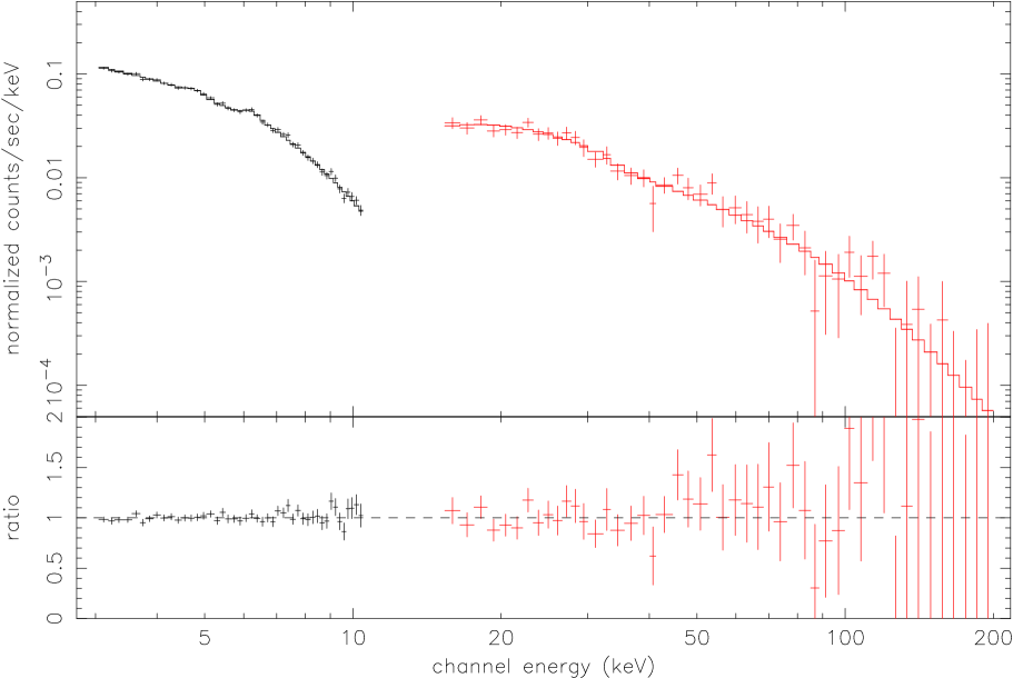
Figure 2: BeppoSAX spectrum of NGC 5548 and the best fit with our model + Fe K$\alpha$ + reflection hump, in the range 3-200 keV (see text).

We then use these same parameter values, by fixing them in the XSPEC procedure, to compare the model (that we have found well fitting the 3-200 keV range) to the whole energy range of BeppoSAX data; the result of this comparison is much worse, giving an unacceptably large value of $\chi_{\nu}^{2}$ ($\sim 16$). In fact, keeping fixed the parameters selected in the restricted energy range (3-200 keV) and “freezing” the normalization constant of the LECS data group to a value such that the ratio of LECS/MECS normalization lies within the acceptable interval (see Fiore et al. fiore (1999)) and, at the same time, such as to make the model match the data in the low energy range ($E\la 0.4$), the model flux $f(E)$ (keV cm^-2 s^-1 keV^-1) that we obtain is instead significantly higher than the unfolded observed spectrum in the range 0.4- 3 keV; this is shown in Fig. 3.

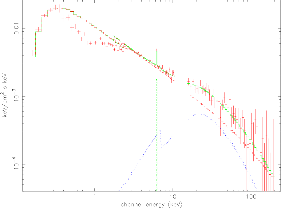
Figure 3: Comparison of BeppoSAX data over the whole energy range observed with the IC “primary” spectrum + Fe line + reflection component as derived from the 3-200 keV best fit: the necessity of some absorption component is apparent from the plot; see the text for further explanation.

This energy range is exactly the one where the expected effects of a warm absorber are most evident (Nicastro et al. 1999a ). Indeed, recent observations of this energy range with the unprecedented spectral resolution of XMM-Newton, have shown an astounding complexity of spectral features, emission and absorption lines, possibly blueshifted, (see Steenbrugge et al. steen (2003); Kaastra et al. kaastra (2002)) revealing how complicated and composite a realistic description of the absorbing gas must be, certainly falling beyond the scope of the present work. In the context of Beppo-SAX data analysis in the “low-energy” spectral region, characterized by a limited spectral resolution (with respect to that of the grating spectrometers on board of XMM), similarly to what is done by Pounds et al. (pounds (2003)), we choose to give an approximate description of the warm absorber effects with a series of absorption edges, namely 5 edges.

We postpone the discussion of these edges until Section 5.3 and at present we only say that including them in the fitting procedure (each of them represented by a multiplicative component zedge in XSPEC), and keeping the IC model spectrum parameter values fixed as those in Table 1, now we obtain a much better fit ($\chi^{2}_{\nu}=0.96$ (133 d.o.f.)) over the entire observed energy range 0.12-200 keV; this is shown in Fig. 4.

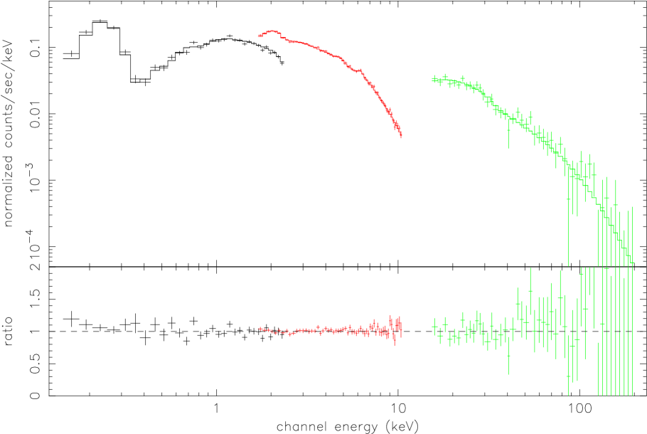
Figure 4: BeppoSAX spectrum of NGC 5548 and the best fit with our model + Fe K$\alpha$ + reflection hump + absorption edges (see text). No soft excess is included.

5.2 Physical parameters for the generation of the IC spectrum

Table 1 shows the best fit values for the parameters defining the physical scenario that we have devised for the generation of the primary X-ray spectrum.

We have also tried to fit models corresponding to different values of $s$ and $\gamma_{\rm o1}$; the ones we have finally chosen, given in Table 1, are those for which the best fit is obtained, i.e. corresponding to one of the lowest obtainable $\chi^{2}$ values. However, it is interesting to note that variations of these two parameters within $\sim 15\%$ of the reported values result in a fit which is still a reasonable one, if not slightly better: for example, for $s=2.5$ the final $\chi^{2}$ value turns out to be even lower than the one found for $s=3$ (see Table 1). Nevertheless, we have preferred and shown the fit obtained for the model corresponding to $s=3$, since in this case the decrease of the spectrum at high energies is steeper than in the case corresponding to $s=2.5$. Regarding the energy range of the injected electron distribution, recent work on electron acceleration due to magnetic reconnection related processes (Lesch & Birk lesch (1997); Schopper et al. schop (1998)) in the AGN context and, even more specifically, in the AGN corona context, has shown that such processes guarantee acceleration up to maximum energies around $\gamma\sim 2000$, which is essentially in accordance with our choice of the upper limit of the energy range of the initial injected electron distribution.

The values of $R_{\rm UV-X}$ and $N_{\rm tot}$ reported in Table 1 have been directly derived from the best fit procedure. In the hypothesis that approximately one tenth of the coronal volume is flaring at the same time and that the emission is due to a series of $q=10$ almost simultaneous flares, the characteristic linear scale of a typical emitting region can be estimated as $R_{\rm em}\simeq R_{\rm UV-X}/(10q)^{1/3}\simeq\leavevmode\nobreak\ 2.15\times 10^{13}$ cm and the corresponding minimum variability time scale is $\sim\leavevmode\nobreak\ 7.2\times 10^{2}$ s, in accordance with the the data reported by Chiang et al. (chiang (2000)). In this framework the density of non-thermal electrons can be evaluated as

$$n_{\rm rel}\simeq{N_{\rm tot}\over 10(4\pi/3)R_{\rm em}^{3}}\simeq 1.28\times 10^{8}\leavevmode\nobreak\ {\rm cm}^{-3}$$

and the associated optical depth to (non-thermal relativistic) electron scattering is $\tau_{\rm rel}\equiv n_{\rm rel}\sigma_{\rm T}R_{\rm em}\simeq 1.8\times 10^{-3}$. With such a low optical depth, secondary inverse Compton scattering effects can be safely neglected. The computation of how many double scattered photons attain $E=300$ keV shows that their number is significantly lower than that of the photons that have been scattered only once.

Finally, we want mention that a similarly good fit from our model can be obtained also for larger values of $R_{\rm UV-X}$, and, correspondingly smaller magnetic field values, as noted at the end of Section 4.3. In particular, for $B=120$ gauss, from the fit in the 3-200 keV range, we obtain $\chi^{2}_{\nu}=0.76$ (87 d.o.f.), for $R_{\rm UV-X}=(6.0_{-0.01}^{+0.03})\times 10^{14}$ cm and $N_{\rm tot}=(1.40_{-0.01}^{+0.01})\times 10^{51}$ electrons, with essentially the same resulting parameters for the iron line, and with $R=0.8$ and $(0.67_{-0.13}^{+0.13})$ for the cosine of the inclination angle for the pexrav component, defining the reflection component of the spectrum. Extending the fit to the whole energy range of BeppoSAX data in the same way described in the previous section, we obtain $\chi^{2}_{\nu}=0.95$ (132 d.o.f.), thus giving as good a fit as the one described in the previous Section. For this case $R_{\rm em}\simeq 1.29\times 10^{14}$ cm, so that the relativistic electron density is $n_{\rm rel}\simeq 1.56\times 10^{7}\leavevmode\nobreak\ {\rm cm}^{-3}$, and the associated optical depth to scattering is $\tau_{\rm rel}\simeq 1.3\times 10^{-3}$. Nevertheless, we have chosen to fully illustrate the fit corresponding to $R_{\rm UV-X}=1\times 10^{14}$ cm in the previous and in the present Sections, following the outcomes of the discussion of Section 2 regarding the estimate of the typical scale length of active loops, which indicate that smaller size coronal loops are favoured.

5.3 Other components of the observed X-ray spectrum

We want to mention here that the fit we have obtained seems to indicate that no significant soft excess is required from the 2001 data we have analyzed. This might seem in disagreement with Pounds et al. (pounds (2003)) (who detect an “apparently unambiguous excess of soft X-ray flux below 0.7 keV”); however, this is only apparent, since their conclusion comes from the use of a simple power-law to describe the primary spectrum. On the contrary, in our case the X-ray primary spectrum itself is the result of inverse Compton reprocessing of soft photons by our evolving non-thermal distribution of relativistic electrons, and, as such, turns out to be characterized by a more complex behaviour. Specifically, it shows a slight hump right in the energy region around and below $\sim$ 1 keV, as it is suggested by Fig. 1 and could be better seen with a more appropriate scale. This is just the time-averaged effect of the evolution of the lower limit of the electron energy distribution, $\gamma_{1}=\gamma_{1}(t)\leq\gamma_{\rm o1}$, and it turns out to be essentially enough to suppress the necessity of an additional soft excess component. We note, however, that we might indeed “force” a soft excess component in the framework of our model and still obtain a reasonable fit; in other words, we do not exclude the possibility of a soft excess component, but we stress again that it turns out to be not necessary to introduce it within our modeling scenario.

Let us briefly discuss the XSPEC components that we have added to our resulting IC spectrum. In fact, we have introduced these components since it is well known that they do have an influence on the “low” X-ray energy range for what regards the warm absorber, and in the medium-to-high energy range for the Iron emission line and the reflection hump (Nicastro et al. nica (2000); Petrucci et al. petru (2000)); as a consequence, to fit the whole BeppoSAX energy range it is necessary to account for them. However, we want to stress that we are not interested here in discussing the nature/origin of these reprocessing components in detail, but instead we want to put emphasis on the feasibility of an “intrinsic” emission model such as the one we have envisaged. Furthermore, the parameters we obtain from the general fit for the warm absorber and for the other reprocessing components are not in disagreement with the values cited in pre-XMM analyses in the literature (Nicastro et al. nica (2000); Pounds et al. pounds (2003)).

As for the five absorption edges through which we give a simplified description of the warm absorber effects, four of these edges have been fixed to the theoretical OVII, OVIII and NeIX/X and MgX/XI edge energy values (and these are essentially the four edges mentioned by Pounds et al. (pounds (2003))). The fifth edge, which is required if we want to obtain a good fit, turns out to be placed at $\la 0.5$ keV, and it could correspond to the deep absorption edge of CIV predicted by photoionization models of the warm absorber (see Nicastro et al. 1999a , 1999b ). However, what is of interest to our present purpose is that we do obtain a good fit by allowing for absorption edge energies and resulting optical depth values which are in accordance with published studies of warm absorbers prior to the high energy resolution observations of XMM. In fact, this allows us to devote our attention to the “primary” X-ray continuum as emitted in the non-thermal scenario we have devised. Moreover, it is not very meaningful any longer to dwell on the meaning and origin of “low-energy” spectral features as they appear from BeppoSAX data, since CHANDRA and XMM, allowing for much higher spectral resolution and therefore much more detail, have now provided a much more complex picture, revealing a richness of lines and spectral features whose analysis requires a different approach and different means of study, and, possibly, showing no evidence at all for the oxygen edges previously identified in lower energy resolution observations (Kaastra et al. kaastra00 (2000)).

6 Application of the model to AGN X-ray sources: general considerations

In the previous section we have shown that the X-ray spectrum of the specific Seyfert 1 source NGC 5548 can be interestingly well explained by the non-thermal and intrinsically non-stationary model that we have devised. Now we turn our attention to the analysis of the descriptive capability of the model with respect to a few general observed trends and properties of Seyfert 1’s X-ray spectra. We do not get into the detailed and quantitative description of a fit, like we did in the previous two sections; in fact, since in our model the reprocessed spectrum depends on the input soft radiation spectrum, and on the loop magnetic field through the locally generated synchrotron component, which represents a seed component for inverse Compton reprocessing as well, to compare its outcome with the average Seyfert 1 X-ray spectrum, we should have defined an averaged opt.-UV spectrum to be reprocessed and an average magnetic field, and then fit the resulting X-ray spectral distribution to the “averaged” observed spectrum, obtaining values of the physical parameters coming into play that would define “average” physical properties of the emitting regions. As a matter of fact, especially because of the significant dependence of these parameters on the physical condition of the very central region of the AGN, i.e. on the effective value of the central black hole mass ultimately, a procedure of this kind would, in our opinion, lead to not very meaningful results. On the contrary, we point our attention to the capability of our model to reproduce a very general spectral characteristic of the observed Seyfert X-ray spectra, that is the relatively small dispersion of the distribution of the spectral index $\alpha$ of a power-law like description of the “primary” spectral flux ($f(E)\propto E^{-\alpha}$) at least in the energy range $\sim 2-10$ keV around an average value $\alpha\sim 0.9$ (Nandra & Pounds nandra94 (1994); Nandra et al. 1997a ; Zdziarski et al. zdz95 (1995); Zdziarski et al. zdz00 (2000); Gondek et al. gondek96 (1996); Matt matt01 (2001) for BeppoSAX broad-band observations), by now considered as a “canonical” value. It is appropriate to note here that, strictly speaking, such an inference on the primary spectrum is somewhat model dependent, since the “canonical” value $\alpha=0.9$ is obtained fitting the observed spectrum with a series of components (primary and reprocessed, see also Section 5.1) that are a priori supposed to be descriptive of the general mechanisms at work in the definition of the resulting X-ray radiation. In particular, the existence of a reflection component turns out to be determinant; for an interesting, and in a way “historical”, analysis of the developments of the global phenomenological understanding of X-ray spectra of Seyfert 1 nuclei, we refer for example to Nandra & Pounds’s (nandra94 (1994)) work on GINGA data, showing that the strong flattening of the spectrum in the 10-18 keV range, with respect to the 2-10 keV behaviour, was well accounted for by introducing a reflection component in the spectral fitting, thus giving a relatively narrow distribution of values of the spectral index of the power-law description of the primary spectrum around an average value $\sim 0.9$.
Back to the point, it is our purpose to show that our model can quite generally reproduce a spectrum that fairly well approximates a power-law behaviour in the range 2-10 keV with a spectral index that does match the relatively narrow range of values around $\alpha=0.9$ inferred from the general interpretation of Seyfert X-ray spectra observations. In fact, we restrict our analysis to the energy interval delimited by $\sim$ 2 and 10 keV respectively because of two orders of reasons, which we explain in the following and are anyway intimately connected with each other. Indeed, on one hand our model primary spectrum, when considered on a much broader X-ray energy range (such as the one observed by BeppoSAX), necessarily (i.e. due to its origin) is much more complex than a simple power-law. On the other hand, within the general interpretative framework, with the exception of the generally narrow (see Bianchi et al. bianchi04 (2004)) Iron line at $\sim 6.4$ keV, the effects of the reprocessing components usually accounted for in the theoretical explanation of the resulting broad-band X-ray spectrum are expected to be much more conspicuous outside of this $\sim 2-10$ keV range, (because of absorption on the lower-energy side, and of reflection on the higher-energy side). Therefore, outside of the $2-10$ keV range, deviations of our model spectrum from a simplistic power-law behaviour are mixed up with reprocessing features/distortions and can be disentangled only by altogether fitting the observed spectrum, possibly giving sort of different results for the reprocessing component parameters (with respect to the simple primary broad-band power-law description) but in no way rejectable on a theoretical basis. Keeping in mind the discussion above, to attain our goal, we have chosen the following procedure. First, we had to define some sort of “average” properties of a typical Seyfert 1 spectrum in the optical-UV range. Several works in the literature attempt to define these properties for the general category of radio-quiet AGNs, or for QSOs only (see for example Risaliti & Elvis risaliti04 (2004) and references therein), but, in order to select an average opt.-UV spectral behaviour more specifically referring to the class of Seyfert 1s, we referred to Koratkar & Blaes’s (korat99 (1999)) work, specifically to their Fig. 1, in which the authors show an average SED (spectral energy distribution) for Seyfert 1s, distinguishing it both from radio-quiet quasars (QSOs) and radio loud ones. Approximately fitting a opt.-UV Sy-1 spectrum from Koratkar & Blaes’s (korat99 (1999)) Fig. 1, we computed a grid of resulting primary X-ray spectra from our model, changing the physical parameters that we found more significant in the detailed fitting of NGC 5548’s X-ray BeppoSAX spectrum as performed in Section 5, namely $R_{\rm UV-X}$ and $N_{\rm tot}$, together with the magnetic field in the active region, $B$. We find that, for a reasonable range of $N_{\rm tot}$ values, and for a given $R_{\rm UV-X}$, we can quite easily define a range of values of the magnetic field $B$ corresponding to which our model spectrum in the range 2-10 keV can be well described as power-law like, with spectral index $\alpha$ values between 0.85 and 0.95. To quantify our assertion, for example, this typical slope range for the power-law best describing our spectrum can be obtained for $B\simeq 100-200$ gauss, when $R_{\rm UV-X}=6\times 10^{14}$ cm, whereas for $R_{\rm UV-X}=1\times 10^{14}$ cm this same $\alpha$-range is reproduced for $B\simeq 400-600$ gauss. This is in accordance with the trend that we have briefly discussed at the end of Section 4.3, referring to the specific fitting of NGC 5548’s BeppoSAX spectrum; in fact, we do find that, even “starting” from an an average opt.-UV spectrum to be IC reprocessed by the coronal relativistic electrons, an increase of the coronal structure extension requires smaller values of the magnetic field to reproduce the canonical power-law slope, i.e. to better fit observed spectra.

Another issue we have to confront with is X-ray variability, its general behaviour and its relationship with variability properties at other wavelengths. X-ray spectral variability studies have shown that many Seyfert spectra soften when the continuum flux increases (Nandra et al. 1997b ; Markowitz & Edelson mark01 (2001); Markowitz et al. mark03 (2003)). Also in NGC 5548 temporal variability has been observed at several wavelengths; in particular, UV-EUV and simultaneous X-ray variability data are available (Chiang et al. chiang (2000); Haba et al. haba (2003); Kaastra et al. kaas2004 (2004)), and the same trend, namely an UV-EUV intensity increase larger than the X-ray one, is present. Another characteristic behaviour which appears both in NGC 5548 (Chiang et al. chiang (2000); Kaastra et al. kaas2004 (2004)) and also in some other sources (see, e.g., McHardy et al. hardy (2004); Blustin et al. blustin (2003)) is the fact that hard X-ray intensity variations show a delay with respect to the soft X-ray ones.

A detailed comparison of our model results with the observed variability properties is out of the purpose of this paper. However, it is important to understand whether our model could reproduce the most relevant variability trends outlined above. In our model both an increase in the magnetic field intensity and a different geometry, i.e. less numerous but more extended active loops, can easily reproduce a softening of the spectrum. More specifically, an increase of the magnetic field intensity of 25% can induce an increase in the observed spectral luminosity of 22% at 0.3 keV and of 7% at 3 keV, while a decrease of the number of active regions from ten to three can induce an increase in the observed spectral luminosity of 28% and 10%, respectively corresponding to the same two energy values cited above. A non-homogeneous magnetic field showing different geometrical configuration and intensity in different regions of the accretion disk, owing to the disk rotation and to its intrinsic temporal variability, would produce changes such as the ones mentioned above in the coronal magnetic structure and in the number and properties of flaring loops. This picture is in accordance with the idea of Kaastra et al. ( kaas2004 (2004)) regarding the possible presence of a large hot active region above the disk. In this context, magnetic field properties can be imagined to evolve in time in such a way to justify the observations of the hard X-ray part of the spectrum still increasing, while the soft one decreases, in accordance with the reported time lag of hard X-ray radiation.

7 Discussion and Conclusions

In this paper we have developed the idea that AGN coronae resemble the stellar ones, where flares powered by magnetic reconnection inject accelerated electrons into magnetic, loop-like, structures. In this framework, X-ray emission from AGNs is due to the non-thermal, time-evolving distribution of relativistic electrons and the dominant emission mechanism is inverse Compton scattering of IR-UV soft radiation emitted by the underlying accretion disk. The model has been tested on one of the brightest Seyfert 1 galaxies, NGC 5548.

Despite making exceedingly simplifying assumptions, our model gives a very good fit to the X-ray spectrum of NGC 5548 (see Figs. 2 and 4) as observed by BeppoSAX in July 2001, with physically reasonable values of the model parameters. In addition, the spectral index of the initial electron energy distribution, $s$, that we derive turns out to be quite in accordance with the values inferred for solar flares, hence supporting the idea that magnetic reconnection is related to the electron acceleration mechanism. Moreover, our $R_{\rm UV-X}\simeq 4.8R{\rm{}_{S}}$ is substantially consistent with the characteristic size of a coronal structure for an object like NGC 5548. If ten flares are active at the same time in the corona (see Sect. 5), the estimated size of the blob-like structure implies that significant variations in the observed luminosity are on time-scales longer than $\sim 7.2\times 10^{2}$ s, an estimate which is in accordance with X-ray luminosity variations observed up to now (Chiang et al. chiang (2000); Nicastro et al. nica (2000)). Since our model is based on a time-evolving emission process, possible variations of the number of active flares and of their intensity allow to decouple X-ray intensity variations from the UV ones and also to reproduce the observed changes in the emission spectrum (see section 6). Another advantage of our model is that it does not require the introduction of a soft X-ray emission component, since the model itself reproduces the so called “soft excess” (see Sect. 5.3).

A qualitative comparison with general trends inferred from observations of the X-ray spectra of Seyfert 1 active nuclei has been discussed in Section 6: both the “average” spectral index $\alpha\simeq 0.9$ generally determined for power-law approximations of the “primary” spectrum and the variability patterns observed for several sources (and in particular for the one, NGC 5548, we analyzed in more detail) briefly described in the previous Section can be rather easily reproduced in the framework of our model. This is encouraging in what concerns the feasibility of the scenario we propose in the present work.

As outlined in the introduction, two main different families of models have been developed in order to understand the physics of the X-ray emitting plasma: those in which the energy distribution of the electrons responsible for X-ray emission is thermal and those in which it is instead non-thermal. It is interesting to highlight the most important points distinguishing the presently proposed scenario from the above cited families of models. Differences with thermal models are straightforwardly identified, since our model is based on the impulsive injection of highly relativistic electrons non-thermally distributed in energy (and evolving in time due to their energy losses), interacting with seed soft photons to produce a time dependent X-ray spectrum through a single-scattering inverse Compton process. On the contrary, the usual thermal models are characterized by a steady-state trans-relativistic thermal energy distribution for the electrons, which interact with the soft radiation field again through the inverse Compton mechanism, but in a multiple scattering process, thermal Comptonization, with each one of the scatterings involving a relatively small amount of energy exchange. In our scenario we do allow for an “underlying” thermalized coronal plasma component, but its physical properties differ from those of “thermal models” quite significantly, as discussed in Sect. 4.3; in particular, the density of the thermalized component is much lower than that estimated for thermal models. As a consequence, since the optical depth to scattering of this component is much smaller than one, no significant effect from the Compton interaction between thermal matter and photons can be expected, not even Compton “recoil” (see Sect. 4.3). The “primary” spectrum is therefore only determined by the non-thermal relativistic electron interactions with the radiation field.

To this respect, it is also important to stress the properties of our coronal emitting component, i.e., of the non-thermal relativistic electron population. In fact, also this component is optically thin to scattering, since its Thomson optical depth is very low ($\sim 0.0018$ for the case of NGC 5548), and this justifies our choice of a simple single-scattering description.

Concerning the “standard” stationary non-thermal models (see Svensson sv94 (1994); Ghisellini ghise94 (1994)), two main differences with respect to our present model can be identified and are discussed in the following; however, it is important to notice that these same two differences also apply to the comparison with stationary thermal Comptonization models mentioned above.

The first significant difference is the fact that our model is intrinsically non-stationary and the evolution in time of the resulting spectra (as it has been shown in Section 4.2) turns out to be a decisive factor in order to reproduce the observed steepening of the X-ray spectrum above 100 keV, in accordance with OSSE and BeppoSAX results.

Secondly, the compactness parameter (see below for its explicit definition, as given by Guilbert et al. guilbert (1983)), consistently evaluated for the coronal emitting regions in our scenario, is lower than the critical limit for pair production to be significant, thus avoiding, in our case, the problem of the annihilation line, generally expected from standard, stationary non-thermal models, but not detected by OSSE (Johnson et al. johnson97 (1997); Zdziarski et al. zdz97 (1997)). In fact, following Guilbert et al. (guilbert (1983)), the compactness parameter of the coronal structure can be estimated as $l_{\rm corona}\sim\sigma_{\rm T}/(m_{\rm e}c^{3})(L_{\rm X}/R_{\rm UV-X})$, where $L_{\rm X}$ is the source X-ray luminosity and $R_{\rm UV-X}$ is the global extent of the region where the IC reprocessing occurs. Using for $L_{\rm X}$ values in the range $2-3\times 10^{43}$ erg/s (as reported by Nicastro et al. nica (2000), Perola et al. perola02 (2002), Bianchi et al. bianchi04 (2004) for NGC 5548), we get an estimate $l_{\rm corona}\sim 4.9-7.4$, reasonably below the well known limit for pair production to become effective, namely $l\ga 4\pi$. Even lower values can be estimated for the compactness parameter for the single emitting loop (the “direct” analogue of the “blob” of Haardt et al. hmg94 (1994)), since in that case we have $l_{\rm loop}\sim\sigma_{\rm T}/(m_{\rm e}c^{3})(L_{\rm X}/q)/R_{\rm em}\sim 2.3-3.4$, to be compared with the reference value $\sim 30$ of Haardt et al. (hmg94 (1994)). Therefore, in our framework neglecting pair production/annihilation effects on the spectrum turns out to be fully justified from the resulting conditions of the emitting structure, and this supports the consistency of our treatment. It is also noteworthy that this condition differentiates our model from the thermal Comptonization ones as well, as it is clear from the comparison above with compactness properties of the thermal “patchy-corona” model of Haardt et al. (hmg94 (1994)).

Still referring to the issue of a comparison of our presently proposed scenario with preexistent models, we have to mention that models including both a thermalized (Compton efficient) electron population and a non-thermal relativistic component have been also devised; these models have been developed to account for the fact that a purely thermal (Maxwellian) distribution for energetic electrons is quite difficult to achieve (see Coppi coppi99 (1999)).

On one hand thermalization mechanisms, which are more efficient than Coulomb collision for energy exchange, have been explored, although, according to Coppi (coppi99 (1999)), “realistic calculations are in general quite difficult, especially near an accreting black hole, where we still have relatively poor knowledge of the exact physical conditions”. It is far beyond the scope of the present paper to analyze this topic in detail; we just mention one interesting model belonging to this first sub-class, namely the so-called “synchrotron boiler”, devised by Ghisellini et al. (ggs88 (1988)) and further developed by Ghisellini et al. (ghs98 (1998)), based on efficient self-absorption of synchrotron photons, emitted by electrons in the source, by different electrons of the same population, thus “rapidly” exchanging energy and producing relaxation of the particle population itself to a resulting steady-state quasi-Maxwellian distribution, with a high-energy tail. It is important to notice that the main assumptions for this mechanism to be efficient, and thus for thermalization to effectively occur (Ghisellini et al. ghs98 (1998)), are that i) the mean energy, $<\gamma>$, of the energetic electrons is just a few, and ii) the magnetic energy density is dominant with respect to the radiation energy density, together with the further condition that the soft photons to be Comptonized only arise from the reprocessing of about half of the hard radiation by cold (disk) matter close to the active (Comptonizing) region. None of these conditions is met in our scenario, in which no such straightforward and stringent relation between the external soft radiation energy density and the hard (i.e. X-ray) one is required, thus allowing our magnetic energy density to be somewhat lower than the soft seed radiation energy density, and in any case not dominant (even though magnetic energy is in our view the reservoir for the electron impulsive energization, and, therefore, ultimately, for the high energy emission); moreover, contrary to assumption i), mentioned above, for the thermalization mechanism to be efficient, the accelerated electrons we consider are characterized by much higher electron energy ($\gamma_{\rm min}\gg 1$).

On the other hand, models intrinsically allowing for a “lower” energy portion of the electron distribution of a Maxwellian form and a steady injection of high energy electrons in a power-law or delta-function distribution have also been devised (Coppi coppi99 (1999)). These are the so-called hybrid thermal/non-thermal models and the resulting steady state distribution is in fact a Maxwellian plus a high energy non-thermal tail, whose relative importance depends basically on the ratio of the power supplied to the thermalized component (heating rate) and the power injected in non-thermal electrons ($l_{\rm th}/l_{\rm nth}$ in terms of compactnesses) as well as on the non-thermal injection spectrum (especially the characteristic $\gamma$ range). As a consequence, the resulting high energy spectrum depends on these parameters as well. It is well known (see Ghisellini et al. ghf93 (1993)) that, as long as the radiative process is multiple Compton scattering and the maximum particle energy is a few MeV, the resulting high energy photon spectrum is indistinguishable from the thermal expected one, and is basically independent of the details of the distribution of particles. When the $\gamma_{\rm max}$ of the non-thermal electrons is instead quite high, the spectral properties will depend on the ratio $l_{\rm th}/l_{\rm nth}$, but, even when this ratio is $\gg 1$, the spectrum should be distinguishable from the thermal one at gamma-ray energies. These models are at present mostly applied to galactic black holes in their soft states, that cannot be fitted by the thermal models, since the corresponding spectra do show power-law like tails at least up to 1 MeV (although relatively weak), and, as a consequence, appear to require a high energy non-thermal tail in the electron distribution contributing to the formation of the spectrum itself; on the contrary, for X-ray spectra of normal broad-line Seyfert 1 active nuclei, thermal Comptonization models have been preferred, up to now. It is appropriate, here, to cite a significant statement in Coppi’s (coppi99 (1999)) review on hybrid models, again enlightening a substantial difference with our presently proposed scenario: the spectra produced by Coppi’s code for hybrid models are “steady state, while the real spectra that are being fit are typically time integrations over many flares…”.

In the light of all the arguments above discussed, we can conclude that while the comparison of our model with observations suggests that our model is plausible and can be considered a valid alternative to thermal Comptonization models, a deeper analysis is still necessary to fully understand the physics of the emitting medium in AGN coronae.

- (1) Bianchi, S., Matt, G., Balestra, I., Guainazzi, M.,& Perola, G.C. 2004, A&A 422, 65
- (2) Blumenthal, G.R., & Gould, R.J. 1970, Rev. Mod. Phys., 42, 237
- (3) Blustin, A.J., Branduardi-Raymont, G., Behar, E., et al. 2003, A&A 403, 481
- (4) Boella G., Butler R., Perola G., et al. 1997a, A&AS, 122, 299
- (5) Boella G., Chiappetti L., Conti G., et al. 1997b, A&AS, 122, 327
- (6) Brotherton, M.S., Green, R. F., Kriss, G. A., et al. 2002, ApJ, 565, 800
- (7) Carleton, N.P., Elvis, M., Fabbiano, G., et al. 1987, ApJ, 318, 595
- (8) Chiang, J., Reynolds, C. S., Blaes, O. M., et al. 2000, ApJ, 528, 292
- (9) Coppi, P. S. 1999, in High Energy Processes In Accreting Black Holes, ed. J. Poutanen & R. Svensson (San Francisco: ASP), ASP Conf. Ser. 161, 375
- (10) Di Matteo, T. 1998, MNRAS, 299, L15
- (11) Dove, J.B., Wilms, J., & Begelman, M.C. 1997, ApJ, 487, 747
- (12) Fiore F., Guainazzi M., & Grandi P. 1999, Cookbook for B͡eppoSAX Spectral Analysis
- (13) Frontera F., Costa E., Dal Fiume D., et al. 1997, A&AS, 122, 371
- (14) Galeev, A.A., Rosner, R., & Vaiana, G.S. 1979, ApJ, 229, 318
- (15) Ghisellini, G., Guilbert, P., & Svensson, R. 1988, ApJL, 335, L5
- (16) Ghisellini, G., Haardt, F., & Fabian, A.C. 1993, MNRAS, 263, L9
- (17) Ghisellini, G. 1994, in “Frontiers of Space and Ground-Based Astronomy”, eds. Wamsteker, W., Longair, M.S., & Kondo, Y., p. 347, Kluwer Academic Publishers, Dordrecht: The Netherlands
- (18) Ghisellini, G., Haardt, F., & Svensson, R. 1998, MNRAS, 297, 348
- (19) Ghisellini, G., Haardt, F., & Matt, G. 2004, A&A, 413, 535
- (20) Ginzburg , V.L. 1969, Elementary processes for cosmic ray astrophysics, Gordon and Breach
- (21) Gondek, D., Zdziarski, A. A., Johnson, W. N., et al. 1996, MNRAS, 282, 646
- (22) Guilbert P.W., Fabian A.C., & Rees M.J. 1983, MNRAS, 205,593
- (23) Haardt, F., & Maraschi L. 1991, ApJL, 380, L51
- (24) Haardt, F., & Maraschi L. 1993, ApJ, 413, 507
- (25) Haardt, F., Maraschi, L. & Ghisellini, G. 1994, ApJL, 432, L95
- (26) Haardt, F. 1997, Mem. Soc. Astron. It., 68, 73
- (27) Haba, Y., Kunieda, H., Misaki, K., et al. 2003, ApJ, 599, 949
- (28) Heyvaerts, J.F., & Priest, E.R. 1989, A&A, 216, 230
- (29) Johnson, W. N., McNaron-Brown, K., Kurfess, J. D., et al. 1997, ApJ, 482, 173
- (30) Kaastra, J.S., Mewe, R., Liedhal, D. A., Komossa, S., & Brinkmann, A. C. 2000, A&A, 354, L83
- (31) Kaastra, J.S., Steenbrugge, K. C., Raassen, A. J. J., et al. 2002, A&A, 386, 427
- (32) Kaastra, J.S., Steenbrugge, K. C., Crenshaw, D. M., et al. 2004, A&A 422, 97
- (33) Klein, K.-L., Aurass, H., Soru-Escaut, I., & Kalman, B. 1997, A&A, 320, 612
- (34) Koratkar, A., & Blaes, O. 1999, PASP, 111, 1
- (35) Krolik, J.H. 1999, Active Galactic Nuclei, Princeton University Press
- (36) Lang, K.R. 1980, Astrophysical Formulae, Springer Verlag
- (37) Lesch, H., & Birk, G.T. 1997, A&A, 324, 461
- (38) Liang, E.P.T, & Price, R.H. 1977, ApJ, 284, 247
- (39) Liang, E.P.T. 1979, ApJL, 231, L111
- (40) Liu, B.F.,Mineshige, S., & Shibata, K. 2002, ApJL, 572, L173
- (41) McHardy, I.M., Papadakis, I. E., Uttley, P., Page, M. J., & Mason, K. O. 2004, MNRAS, 348,783
- (42) Magdziarz, P., & Zdziarski, A.A. 1995, MNRAS, 273, 837
- (43) Markowitz, A., & Edelson, R. 2001, ApJ 547, 684
- (44) Markowitz, A., Edelson, R., & Vaughan, S. 2003, ApJ 598, 935
- (45) Malkan, A.M., & Sargent, W.L.W. 1982, ApJ, 254, 23
- (46) Masuda, S., Kosugi, T., Hara, H., Tsuneta, S., & Ogawara, Y. 1994, Nature, 371, 495
- (47) Matt, G. 2001, in AIP Conf. Proc. 599, X-Ray Astronomy: Stellar Endpoints, AGN, and the Diffuse X-Ray Background, eds. N. E. White, G. Magaluti, & G. Palumbo (New York: AIP), 209
- (48) Merloni, A., & Fabian, A.C. 2001, MNRAS, 321, 549
- (49) Melrose, D.B., & Brown, F.C. 1976, MNRAS, 176, 15
- (50) Miller, K.A., & Stone, J. M. 2000, ApJ, 534, 398
- (51) Nandra, K., & Pounds, K.A. 1994, MNRAS, 268, 405
- (52) Nandra, K., George, I. M., Mushotzky, R. F., Turner, T. J., & Yaqoob, T. 1997b, ApJ, 476, 70
- (53) Nandra, K., George, I. M., Mushotzky, R. F., Turner, T. J., & Yaqoob, T. 1997a, ApJ, 477, 602
- (54) Nicastro, F., Fiore, F., Perola, G. C., Elvis, M. 1999a, ApJ, 512, 184
- (55) Nicastro, F., Fiore, F., & Matt, G. 1999b, ApJ, 517, 108
- (56) Nicastro, F., Piro, L., De Rosa, A., et al. 2000, ApJ, 536, 718
- (57) Parmar A.N., Martin D.D.E., Bavdaz M., et al. 1997, A&AS, 122, 309
- (58) Perola, G.C., Matt, G., Cappi, M., et al. 2002, A&A, 389, 802
- (59) Petrucci, P.O., Haardt, F., Maraschi, L., et al. 2000, ApJ, 540, 131
- (60) Pounds, K., Reeves, J. N., Page, K. L., et al. 2003, MNRAS, 341, 953
- (61) Poutanen, J., & Svensson, R. 1996, ApJ, 470, 249
- (62) Risaliti, G., & Elvis, M. 2004, astro-ph/0407291
- (63) Schopper, R., Lesch, H., & Birk, G.T. 1998, A&A, 335, 26
- (64) Shakura, N.I., & Sunyaev, R.A. 1973, A&A, 24, 337
- (65) Shibata, K., Tajima, T., Steinolfson, R.S., & Matsumoto, R. 1989, ApJ, 345, 584
- (66) Steenbrugge, K.C., Kaastra, J. S., de Vries, C. P., & Edelson, R. 2003, A&A, 402, 477
- (67) Svensson, R. 1994, ApJS, 92, 585
- (68) Svensson, R. 1996, A&AS, 120, 475
- (69) Uttley, P., Edelson, R., McHardy, I. M., Peterson, B. M., & Markowitz, A. 2003, ApJL, 584, L53
- (70) Wamsteker, W., Rodriguez-Pascual, P., Wills, B. J., et al. 1990, ApJ, 354, 446
- (71) Wandel, A., Peterson, B.M., & Malkan, M.A. 2000, ApJ, 526, 579
- (72) Ward, W., Elvis, M., Fabbiano, G., et al. 1987, ApJ, 315, 74
- (73) Zdziarski, A.A., Johnson, W. N., Done, C., Smith, D., & McNaron-Brown, K. 1995, ApJL, 438, L63
- (74) Zdziarski, A.A., Johnson, W.N., Poutanen, J., Magdziarz, P., & Gierlinski, M. 1997, in The Transparent Universe, Proceedings of the 2nd INTEGRAL Workshop, eds. C. Winkler, T.J.-L. Courvoisier, & P. Durouchoux, ESA-SP 382, Noordwijk: ESA, 373
- (75) Zdziarski, A.A., Poutanen, J., & Johnson, W.N. 2000, ApJ, 542, 703