Is the Number of Giant Arcs in $\Lambda{\rm CDM}$ Consistent With Observations?

Abstract

We use high-resolution N-body simulations to study the galaxy-cluster cross-sections and the abundance of giant arcs in the $\Lambda$CDM model. Clusters are selected from the simulations using the friends-of-friends method, and their cross-sections for forming giant arcs are analyzed. The background sources are assumed to follow a uniform ellipticity distribution from 0 to 0.5 and to have an area identical to a circular source with diameter $1\arcsec$. We find that the optical depth scales as the source redshift approximately as $\tau_{1^{\prime\prime}}=2.25\times 10^{-6}/[1+(z_{\rm s}/3.14)^{-3.42}]$ ($0.6<z_{\rm s}<7$). The amplitude is about 50% higher for an effective source diameter of $0.5\arcsec$. The optimal lens redshift for giant arcs with the length-to-width ratio ($L/W$) larger than 10 increases from 0.3 for $z_{\rm s}=1$, to 0.5 for $z_{\rm s}=2$, and to 0.7-0.8 for $z_{\rm s}>3$. The optical depth is sensitive to the source redshift, in qualitative agreement with Wambsganss et al. (2004). However, our overall optical depth appears to be only $\sim$ 10% to 70% of those from previous studies. The differences can be mostly explained by different power spectrum normalizations ($\sigma_{8}$) used and different ways of determining the $L/W$ ratio. Finite source size and ellipticity have modest effects on the optical depth. We also found that the number of highly magnified (with magnification $|\mu|>10$) and “undistorted” images (with $L/W<3$) is comparable to the number of giant arcs with $|\mu|>10$ and $L/W>10$. We conclude that our predicted rate of giant arcs may be lower than the observed rate, although the precise ‘discrepancy’ is still unclear due to uncertainties both in theory and observations.

1 INTRODUCTION

The Cold Dark Matter (CDM) scenario is now the standard model for structure formation. The “concordance” $\Lambda{\rm CDM}$ model (e.g., Ostriker et al. 1995) is supported by many observations, in particular the large-scale structure of the universe (e.g. Jenkins et al. 1998; Peacock et al. 2001; Tegmark et al. 2004) and the cosmic microwave background (e.g., Spergel et al. 2003).

Giant arcs are formed when background galaxies are distorted into long arc-like shapes by the gravitational shear of intervening clusters of galaxies. They are among the most beautiful images on the sky (e.g., see the Hubble Space Telescope [HST] images of A2218, Kneib et al. 1996). As clusters of galaxies are the largest bound structures in the universe, they are at the tail of the mass function of bound structures. The formation of giant arcs therefore critically depends on the abundance and density profiles of clusters. Observationally, the number of giant arcs was first estimated using the Einstein Medium-Sensitivity Survey (EMSS) by Gioia & Luppino (1994). The largest dedicated search for giant arcs in X-ray clusters was performed by Luppino et al. (1999) who found strong lensing in 8 out of 38 clusters. These fractions were confirmed by Zaritsky & Gonzalez (2003) using the Las Campanas Distant Cluster Survey and Gladders et al. (2003) using the Red-Sequence Cluster Survey. A recent extensive analysis of HST images found 104 candidate tangential arcs in 128 clusters with length to width ratios exceeding 7 (Sand et al. 2005). All these recent studies show that giant arcs are quite common in clusters of galaxies.

Earlier predictions of giant arcs use simple spherical models (e.g., Wu & Hammer 1993). However, such models are clearly inadequate, as the ellipticities and substructures of clusters can enhance the lensing cross-section by a large factor (Bartelmann & Weiss 1994; Bartelmann, Steinmetz & Weiss 1995). More recently, Torri et al. (2004) studied the importance of mergers for arc statistics. Wu & Mao (1996) compared the arc statistics in the Einstein-de Sitter universe and $\Lambda$CDM using simple spherical cluster models and found a factor of $\sim 2$ increase in the $\Lambda$CDM model. A much more realistic study was performed by Bartelmann et al. (1998, hereafter B98) who first pointed out that the number of giant arcs in the $\Lambda{\rm CDM}$ model appears to be below the observed rate in clusters by a factor of 5-10. Meneghetti et al. (2000) investigated the effects of cluster galaxies on arc statistics and found that cluster galaxies do not introduce perturbations strong enough to significantly change the number of giant arcs. Flores, Maller & Primack (2000) drew a similar conclusion. Meneghetti et al. (2003) further examined the effect of cD galaxies on the giant arcs and concluded they are insufficient to resolve the discrepancy. Oguri et al. (2003) studied the ability of tri-axial models of dark matter halos to form giant arcs. They concluded that an inner power-law profile of $r^{-1.5}$ can reproduce the observed giant arcs, while the standard NFW profile (Navarro, Frenk, & White 1997) with an inner profile of $r^{-1}$ is unable to match the observations. Bartelmann et al. (2003) and Meneghetti et al. (2005) studied the probability of the formation of giant arcs in galaxy clusters in different dark-energy cosmologies. But the effect is still insufficient. In an important paper, Wambsganss et al. (2004) pointed out the simple fact that the probability of high lensing magnifications is very sensitive to the assumed source redshift. For example, a source at $z_{\rm s}=1.5$ has a factor of $\sim 5$ higher optical depth than a source at redshift $z_{\rm s}=1$. As the redshift distribution for the background source population that forms arcs is not well known, this introduces an uncertainty in the comparison between observations and predictions.

In this paper, we use high-resolution simulations to re-examine the predicted number of giant arcs and compare our predictions with observations. The outline of the paper is as follows. In §2, we discuss the numerical simulations we use and the method we employ to identify giant arcs in simulated clusters. In §3, we present the main results of the paper and compare them with several previous studies (Bartelmann et al. 1998; Wambsganss et al. 2004; Dalal et al. 2004). In particular, we confirm the results of Wambsganss et al. (2004; see also Dalal et al. 2004) that the predicted arc number is sensitive to the assumed source redshift distribution. However, our overall optical depth appears to be lower than these previous studies, sometimes by a large factor. We examine in detail how the differences arise. This reduction makes it somewhat difficult to match the observed high frequency of giant arcs with our predictions.

In §4, we summarize our results and discuss areas for future improvements.

2 Methods

2.1 Numerical Simulations

The cosmological model considered here is the current popular $\Lambda$CDM model with the matter-density parameter $\Omega_{\rm m,0}=0.3$ and the cosmological constant $\Omega_{\Lambda,0}=0.7$. The shape parameter $\Gamma=\Omega_{\rm m,0}h$ and the amplitude $\sigma_{8}$ of the linear density power spectrum are taken to be 0.21 and 0.9, respectively, where $h$ is the Hubble constant in units of $100\,\rm km\,{s}^{-1}\,\rm Mpc^{-1}$ and we take $h=0.7$. A cosmological N-body simulation with a box size $L=300h^{-1}\,\rm Mpc$, which was generated with our vectorized-parallel $\,\rm P^{3}M$ code (Jing & Suto 2002; Jing 2002), is used in this paper. The simulation uses $512^{3}$ particles, so the particle mass $m_{\rm p}$ is $1.67\times 10^{10}h^{-1}M_{\odot}$. The gravitational force is softened with the $S2$ form (Hockney & Eastwood 1981) with the softening parameter $\eta$ taken to be $30h^{-1}\,\rm kpc$. The simulation has similar mass and force resolutions as that used by B98, but our simulation volume is 8 times larger, and hence contains $\sim 8$ times more clusters. Compared with the simulations of Wambsganss et al. (2004, hereafter W04), our resolutions are a factor of $6.6$ lower in mass and a factor of 10 lower in the force softening. Since strong arcs are produced mostly at radii $\gtrsim 100h^{-1}\,\rm kpc$ in the lens plane, the resolutions are sufficient (see also Dalal et al. 2004). This is also supported by the comparison of our results with those of W04 which are based on much higher resolution – our predicted number of giant arcs is in reasonable agreement with that of W04 if the arcs are identified with their method (see §3.3.2 and Fig. 7).

Dark matter halos are identified with the friends-of-friends method using a linking length equal to 0.2 times the mean particle separation. The halo mass $M$ is defined as the virial mass enclosed within the virial radius according to the spherical collapse model (Kitayama & Suto 1996; Bryan & Norman 1998; Jing & Suto 2002).

2.2 Lensing Notations

For convenience of later discussions, we outline the notations we will use in the paper. We denote the lensing potential as $\phi$. The mapping from the lens and source plane is given by

$$\overrightarrow{y}=\overrightarrow{x}-\nabla\phi,$$ (1)

and the distortion of images is then described by the Jacobian

$${\partial y_{i}\over\partial x_{j}}=\left(\begin{array}[]{cc}1-\phi_{11}&-\phi_{12}\\ -\phi_{21}&1-\phi_{22}\\ \end{array}\right),$$ (2)

where $(y_{1},y_{2})$ are dimension-less source coordinates in the source plane, and $(x_{1},x_{2})$ are dimension-less image coordinates in the lens plane. The Jacobian matrix is given in terms of the lensing potential by the $2\times 2$ matrix on the right hand side, which involves second-order derivatives of $\phi$ with respect to $x_{1}$ and $x_{2}$. The eigenvalues of the Jacobian matrix are denoted as $\lambda_{1}$ and $\lambda_{2}$. Without losing generality, we will assume $|\lambda_{1}|\geq|\lambda_{2}|$. The (signed) magnification is given by

$$\mu={1\over\lambda_{1}\lambda_{2}}.$$ (3)

For an infinitesimal circular source, the length to width ratio is simply given by

$${L\over W}={{1/|\lambda_{2}|}\over{1/|\lambda_{1}|}}=\lambda_{1}^{2}|\mu|.$$ (4)

Notice that $L/W$ is not equal to $|\mu|$ if $\lambda_{1}$ is not unity.

2.3 Lensing Simulations

The lensing properties of numerical clusters are studied using the ray-tracing technique (e.g., B98; W04). For the source population, we use redshifts ranging from 0.6 to 7 with a uniform interval of 0.4. To calculate the optical depth, we use 20 outputs for the simulated box from redshift 0.1 to 2.35 with a step size of $\sim 0.1$. For each redshift, we select the 200 most massive clusters of galaxies as lenses. Notice that this cluster sample is more than a factor ten larger than the samples used by Bartelmann et al. (1998) and Ho & White (2004), although our redshift samplings are sparser than the most recent study of Torri et al. (2004). For each cluster, we use the particles within a cube with a side-length of two virial radii ($2r_{\rm vir}$). The surface densities are then calculated for three orthogonal projections using the SPH smoothing algorithm (Monaghan 1992) on a $1024\times 1024$ grid. Usually, the kernel size is taken to be $30h^{-1}\,\rm kpc$ (comoving). If the particle number within the kernel is fewer than 64, then we double the kernel size until the particle number is larger than 64. However, for the high density regions, when the particle number is larger than 400 within the kernel, we only use the nearest 400 particles to estimate the density. In order to obtain the lensing potential, we also use a larger grid ($2048\times 2048$) centered on the smaller grid; the surface densities are padded with zeros for all the pixels outside the inner grid. The lensing potential is then obtained using the FFT method (B98). Notice that the larger grid is used to avoid aliasing problems due to periodic boundary conditions.

To perform efficient lensing simulations, we first identify regions of interest in the lens plane that have magnifications exceeding $\mu_{\rm limit}\equiv 2.5$ and regions with $\mu\rm<0$; other regions are unlikely to produce giant arcs with $L/W$ exceeding 7.5. Following B98, we assume the sources have an ellipticity, which is equal to one minus the axis ratio, randomly distributed between 0 to 0.5. Each source has an area $S_{\rm source}$ equal to a circular source with a diameter of $1\arcsec$. To have sufficient numbers of pixels in one image, the resolution in the regions of interest is increased to $0.1\arcsec$ (see below) so that most images have at least $n_{\rm s}=\pi\times 0.5^{2}\times\mu_{\rm limit}/0.1^{2}\approx 200$ pixels.

For the regions identified above, the $1024\times 1024$ (coarse) grid does not provide sufficient resolution. To remedy this, we obtain the lensing potential on a finer grid with resolution of $0.1\arcsec$ using cubic spline interpolation of the surrounding $14\times 14$ coarse grid points. In the same step, we obtain the source position for each grid point, and the corresponding magnification and eigenvalues ($\lambda_{1}$ and $\lambda_{2}$).

Once we obtain the lens mapping for the regions of interest from the lens plane to the source plane, we locate the smallest rectangle with area $S_{\rm box}$ that contains all the mapped pixels in the source plane. We then put sources randomly in this rectangle and obtain their imaging properties. The mapped regions in the source plane usually have irregular shapes, so the rectangle will enclose not only the regions of interest but also some regions that do not satisfy our selection criteria ($\mu\geq\mu_{\rm limit}\equiv 2.5$ or $\mu<0$). To avoid sources that straddle the irregular boundary, we only analyze sources further if they contain at least $n_{\rm s}(\approx 200)$ pixels. In order to sample the regions of arc formation well, a large number of sources are placed randomly inside the regions of interest. The number we generate is given by $n_{\rm source}=9{S_{\rm box}/S_{\rm source}}$, where $S_{\rm source}=\pi\times 0.5^{2}$ in square arc seconds, and usually we have $n_{\rm source}>10^{4}$.

For the pixels contained in a source inside the region of interest, we use the lens mapping already derived to obtain the corresponding image positions, and then use the friends-of-friends method to identify giant arcs. To obtain the $L/W$ ratio, we assume giant arcs can be approximated as ellipses, hereafter we refer to this method as ellipse-fitting. Numerically we find this assumption to be valid for most of our giant arcs. However, some images are irregular and cannot be fitted well by an ellipse. They occur when the source straddles higher-order singularities (such as beak-to-beak) or when the source size is comparable to the caustics. But such cases are rare ($\sim 1\%$) for clusters that contribute most of the lensing cross-sections and will thus not affect our results significantly. To calculate the $L/W$ ratio, we need to identify the center of a giant arc, $x_{\rm center}$, which is first taken to be the center of light. Due to the (curved) arc shape, the center often falls outside the arc itself. To find a better center, we select one half of the image positions that are closest to the current center and then re-calculate the center of light. The process is repeated until the center does not change significantly. We verified visually that this procedure yields reliable centers of giant arcs. Once the center is identified, we then locate the point $x_{1}$ that is the furthest from $x_{\rm center}$, and finally the point $x_{2}$ that is the furthest from $x_{1}$. We fit a circular arc that passes through these three points. The length of the arc is taken to be twice the major axis length of the ellipse, $a$, and the length of the minor axis is taken to be $b=S_{\rm image}/(\pi a)$, where $S_{\rm image}$ is the area covered by the image. The $L/W$ ratio is then simply $a/b$. This procedure is identical to the ellipse fitting method in B98.

In W04, the $L/W$ ratio is approximated by the magnification. In order to obtain the arc cross-sections, the magnification patterns need to be calculated on a grid in the source plane. In W04, each pixel has a size of $1.5\arcsec$. However, we find that this is too large for small clusters in our simulations, so we instead used a grid of $0.1\arcsec$ for all the clusters. We use the Newton-Raphson method to find the image position and its corresponding magnification and eigenvalues. When there are multiple images, following W04, we use only the image with the largest (absolute) magnification. In the following, we will study the validity of two approximate measures of $L/W$, namely the magnification, $|\mu|$, and the ratio of the two eigenvalues, $|\lambda_{1}/\lambda_{2}|$. Under these two approximations, we obtain two corresponding cross-sections, which we will denote as $\sigma_{\mu}$ and $\sigma_{\lambda}$. We will compare these two cross-sections with that obtained through ellipse-fitting, $\sigma_{\rm 1^{\prime\prime}}$. The corresponding optical depths can be obtained by integrating the cross-sections along the line of sight (cf. Eq. 7), and we will denote these as $\tau_{\rm 1^{\prime\prime}}$, $\tau_{\lambda}$ and $\tau_{\mu}$. The subscript $1\arcsec$ indicates that the sources have an effective diameter of $d_{\rm eff}=1\arcsec$. Later we will study lensing cross-sections and optical depths for other effective source diameters, $d_{\rm eff}=0.25\arcsec,0.5\arcsec,1.5\arcsec$, and their cross-sections and optical depths will be labeled accordingly.

3 Results

3.1 Caustics, magnifications and cross-sections

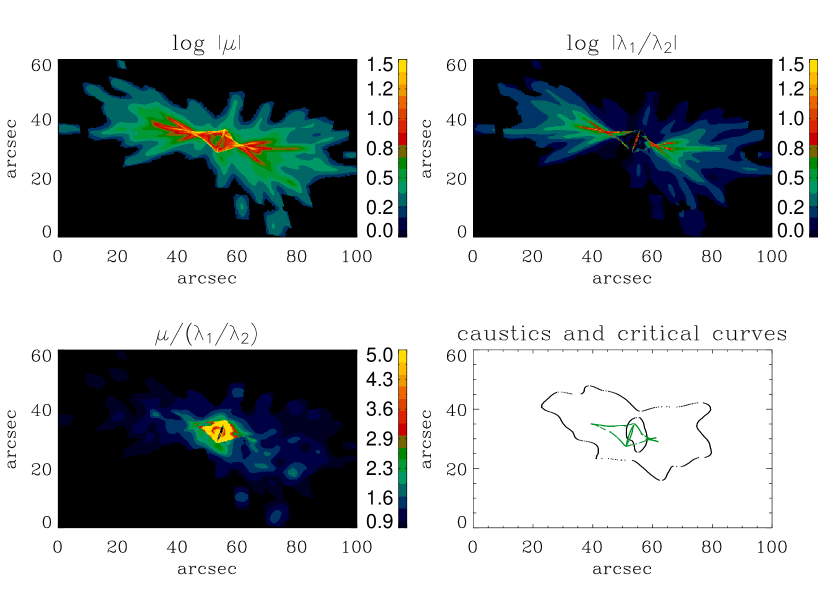
Figure 1: Maps of the absolute magnification (top left), ratio of the two eigenvalues $|\lambda_{1}/\lambda_{2}|$ (top right), $\mu/(\lambda_{1}/\lambda_{2})$ (bottom left), and the caustics and critical curves (bottom-left panel) are shown for the fifth most massive cluster ($M=7.58\times 10^{14}h^{-1}M_{\odot}$) in our simulations at redshift 0.3. The sources are assumed to be at redshift 1.0. The $|\mu|$ and $\lambda_{1}/\lambda_{2}$ values in regions where $0<\mu<2.5$ are set to unity. Pixels with values exceeding the maximum of the color bars are set equal to the maximum.

For illustrative purposes, Fig. 1 shows the lensing properties for the fifth most massive cluster ($M=7.58\times 10^{14}h^{-1}M_{\odot}$) in our simulation at redshift 0.3. The source is at redshift 1. The bottom right panel shows the critical curves and the caustics. The other three panels show the maps of $|\mu|$, $|\lambda_{1}/\lambda_{2}|$ and $\mu/(\lambda_{1}/\lambda_{2})=1/\lambda_{1}^{2}$ in the source plane. Recall that we only consider regions where $\mu>\mu_{\rm limit}\equiv 2.5$ or $\mu<0$. In other regions, we set $\mu$ and $\lambda_{1}/\lambda_{2}$ to unity, which are shown as black in the top left panel. The color bars show the range of the quantities plotted in the maps. Pixels with values exceeding the maximum of the color bar are set equal to the maximum. If we approximate the $L/W$ ratio as either $|\mu|$ or $|\lambda_{1}/\lambda_{2}|$, the top two panels clearly indicate that the cross-section $\sigma_{\mu}$ will be much larger than the cross-section $\sigma_{\lambda}$ for a given length-to-width ratio. This effect is illustrated further in the bottom left panel where we plot the map of $\mu/(\lambda_{1}/\lambda_{2})$. In most cases, especially for the high magnification regions where arcs are expected to form, this ratio is larger than 1, which indicates that for an infinitesimal circular source, $|\mu|$ will over-estimate the $L/W$ ratio. As a check of our lensing simulations, Fig. 2 shows the magnification probability distribution for the cluster shown in Fig. 1. Our results nicely reproduce the asymptotic relation $p(>|\mu|)\propto\mu^{-2}$ expected from the fold caustics when $|\mu|\gg 1$ (e.g., Schneider, Ehlers, & Falco 1992).

To understand why the approximation $L/W=|\mu|$ appears to over-estimate the arc cross-section, we study a cluster with a generalized NFW profile (Navarro, Frenk & White 1997; see also Moore et al. 1998):

$$\rho(r)\propto r^{-\alpha}(r+r_{\rm s})^{-3+\alpha},~{}~{}0<r<r_{\rm vir},$$ (5)

where $r_{\rm s}$ is the scale radius, and $r_{\rm vir}$ is the virial radius. The cluster is at redshift of 0.3 with a mass of $10^{15}h^{-1}M_{\odot}$. The power-law index ($\alpha$) is taken to be 1.5 and the concentration parameter $c=r_{\rm vir}/r_{\rm s}=2.28$ (Oguri 2002). The source redshift is taken to be unity. Fig. 3 shows the relation between $|\lambda_{1}|$ and $|\mu|$ for the minimum, saddle and maximum images in the time delay surface. The tangential arcs are primarily formed by the minimum images while the radial arcs are formed by the maximum images. For an infinitesimal circular source, the $L/W$ ratio is equal to $|\mu|$ multiplied by $\lambda_{1}^{2}$ (see Eq. 4). It is clear that for the minimum image, at high magnifications, $\lambda_{1}\rightarrow 0.65$, while for the maximum image, $\lambda_{1}\rightarrow 1.3$. As for high magnifications, the asymptotic cross-section follows the probability distribution $p(>|\mu|)\propto\mu^{-2}$ (Schneider et al. 1992), the cross-sections for the tangential arcs therefore satisfy $\sigma_{\lambda}\approx{\lambda_{1}}^{4}\sigma_{\mu}\approx 0.18\sigma_{\mu}$. Similarly, for the radial arcs, we have $\sigma_{\lambda}\approx{\lambda_{1}}^{4}\sigma_{\mu}\approx 2.9\sigma_{\mu}$. As the tangential arc cross-section usually dominates over the radial arc cross-section, it follows that the $L/W=|\mu|$ assumption will over-estimate the arc cross-sections by a factor of $\approx 1/0.18=5.6$.

Fig. 4 shows how the cross-section of giant arcs is contributed by clusters with different masses at redshifts 0.3 and 0.2. The background source population is at redshift 1.0. For $z_{\rm l}=0.3$ (right panel), the distribution is peaked around $\sim 8\times 10^{14}h^{-1}M_{\odot}$, and it rapidly declines below $\sim 2\times 10^{14}h^{-1}M_{\odot}$ as the much faster decrease in cross-sections dominates over the rising numbers of low-mass clusters. The cross-section also declines above $M\sim 2\times 10^{15}h^{-1}M_{\odot}$ due the exponential drop in the number of very massive clusters. The left panel is for $z_{\rm l}=0.2$, which can be directly compared with Fig. 4 in Dalal et al. (2004) – the two distributions are roughly consistent with each other.

The ratio of $\sigma_{\rm 1^{\prime\prime}}$ and $\sigma_{\mu}$ is shown in Fig. 5 as a function of the length-to-width ratio ($L/W$) for clusters at redshift 0.3 and background sources at redshift 1.0. The thick line is the cross-section weighted average for the 200 most massive clusters while the thick dashed line shows the result for the generalized NFW model discussed above. The four thin lines are the results for four individual clusters, which are the first, fifth, tenth and fifteenth most massive clusters with $M=1.70\times 10^{15},7.58\times 10^{14},6.55\times 10^{14}$, and $6.02\times 10^{14}h^{-1}M_{\odot}$ respectively.

Recall that $\sigma_{\rm 1^{\prime\prime}}$ is the cross-section calculated using ellipse-fitting, while $\sigma_{\mu}$ is obtained assuming that the $L/W$ ratio is equal to the magnification.

Clearly, the assumption that $L/W=|\mu|$ leads to an over-estimate of the cross-sections by a factor of 7 and 10 for $L/W\geq 7.5$ and $L/W\geq 10$ respectively.

The ratio of $\sigma_{\rm 1^{\prime\prime}}$ and $\sigma_{\lambda}$ is shown in Fig. 6, where $\sigma_{\lambda}$ is again the cross-section calculated assuming $L/W$ to be equal to the ratio of the two eigenvalues. $\sigma_{\rm 1^{\prime\prime}}/\sigma_{\lambda}$ is in the range of 0.5-2 when $L/W$ is in the range of 5-20. Thus, $\sigma_{\lambda}$ offers a better approximation for the arc cross-section than $\sigma_{\mu}$. Notice that the more massive a cluster is or the larger the caustics are, the higher $\sigma_{\rm 1^{\prime\prime}}/\sigma_{\mu}$ and $\sigma_{\rm 1^{\prime\prime}}/\sigma_{\lambda}$ become. This can be understood as follows: as the caustics become larger, the effect of finite source size smoothing decreases. Thus, $\sigma_{\rm 1^{\prime\prime}}$ increases and so do its ratios with $\sigma_{\mu}$ and $\sigma_{\lambda}$.

3.2 Optical depths

To evaluate the optical depth, we first calculate the average cross-section per unit comoving volume:

$$\overline{\sigma}(z_{\rm l},z_{\rm s})={\sum\sigma_{i}(z_{\rm l},z_{\rm s})\over V},$$ (6)

where $\sigma_{i}(z_{\rm l},z_{\rm s})$ is the average cross-section of the three projections of the $i$-th cluster at redshift $z_{\rm l}$, $z_{\rm s}$ is the source redshift, and $V$ is the comoving volume of the box adopted in our lensing simulations. The optical depth can then be calculated as:

$$\tau(z_{\rm s})={{1\over{4\pi{D_{\rm s}}^{2}}}{\int_{0}}^{z_{\rm s}}\,dz\,\overline{\sigma}(z,z_{\rm s})(1+z)^{3}\,{dV_{\rm p}(z)\over dz}},$$ (7)

where $D_{\rm s}$ is the angular diameter distance to the source plane, and $dV_{\rm p}(z)$ is the proper volume of a spherical shell with redshift from $z$ to $z+dz$.

Fig. 7 shows the optical depth as a function of the source redshift, $z_{\rm s}$. Our results can be well fitted by the simple curve

$$\tau_{1^{\prime\prime}}=2.25\times 10^{-6}{1\over 1+(z_{\rm s}/3.14)^{-3.42}}$$ (8)

within 20%.

Fig. 8 shows the differential optical depth as a function of the cluster redshift. For a source at redshift 1, there is little contribution to the optical depth for clusters beyond redshift 0.7, because the critical surface density increases when the lens is close to the source, and very few clusters are super-critical. This trend is in excellent agreement with B98 (see their Fig. 1) and Dalal et al. (2004, see their Fig. 10). For a source at redshift 1, the optimal lensing redshift is around 0.3, which is why we have chosen this redshift to illustrate many of our results for $z_{\rm s}=1$. For a source at redshift 2, the peak shifts to about 0.5. For $z_{\rm s}>3$, the optimal redshift is near 0.6-0.7, and the distributions also become noticeably broader, with a full-width-at-half-maximum of about 0.9. This may have particular relevance to Gladders et al. (2003) who emphasized the lack of lensing clusters with $z_{\rm l}<0.64$ in their sample. There are likely selection biases in the surveys, but we notice that their four (approximate) source redshifts range from 1.7 to 4.9. If such source redshifts are typical for their background galaxies, then the large cluster lens redshift is fully consistent with our predictions. As can be seen from Fig. 8, for sources above redshift 3, most lensing cross-sections are due to lenses below redshift 2.4, and there are wiggles in the optical depth curves. The wiggles around $z_{\rm l}\sim 0.5$ are due to numerical effects as the interval of the lens redshift (where particle positions are dumped from numerical simulations) is large and the numerical integration is not exact. The prominent wiggle around $z_{\rm l}=1.5$ is, however, real. It arises due to significant merger events in our simulations. For sources at high redshift, the cross-sections are dominated by relatively few (most massive) clusters and merger events in these clusters have substantial impact on the cross-section (Torri et al. 2004).

3.3 Comparison with previous studies

Our optical depth turns out to be lower than three previous major studies (B98, W04 and Dalal et al. 2004), by different amounts. We have traced these differences back primarily to the different values adopted for the power-spectrum normalization ($\sigma_{8}$), how the $L/W$ ratio is measured, and whether the numerical simulations have sampled the cluster mass function at the high-mass tail sufficiently. The source size and ellipticity and the matter distribution around clusters also have modest effects on the optical depth. Below we discuss issues in detail.

3.3.1 Comparison with B98

In this study, we have followed closely the methodology of B98. Nevertheless, our optical depth ($3.6\times 10^{-8}$) is roughly $10\%$ of the value found by B98 ($3.3\times 10^{-7}$) for a source population at redshift 1.

Our lower optical depth is mainly due to the lower $\sigma_{8}$ parameter adopted in the current study. In B98, the optical depth was obtained as an average over two sets of simulations, one with $\sigma_{8}=1.12$ and the other with $\sigma_{8}=0.9$. However, the optical depth is dominated by the former, as the clusters in the high $\sigma_{8}$ simulation form earlier and are also more centrally concentrated – both increase the arc cross-section considerably, leading to a higher optical depth than in the current work. Fig. 9 shows the mass function of halos at redshift 0.3 predicted by the extended Press-Schechter formalism (e.g. Sheth & Tormen 2002 and references therein; Press & Schechter 1976). The cluster abundance for $\sigma_{8}=1.12$ is a factor of $\sim 3.5$ higher at $M\sim 10^{15}h^{-1}M_{\odot}$ than that for $\sigma_{8}=0.9$. Even the moderately larger $\sigma_{8}$ adopted by W04 (0.95) leads to a 50% increase in the abundance of clusters at at $M\sim 10^{15}h^{-1}M_{\odot}$ than that for $\sigma_{8}=0.9$, which can increase their optical depth relative to ours (see the end of §3.3.2).

3.3.2 Comparison with W04

The method used by W04 is quite different from ours. They adopted a multiple-lens plane approach, modeling the universe with a three-dimensional matter distribution. In our study, we assume that the formation of giant arcs is dominated by individual clusters, and the large-scale structure along the line-of-sight is not important. As mentioned above, another key difference between our study and W04 is how the $L/W$ ratio is measured: W04 assume the $L/W$ ratio to equal the magnification, while we measure the $L/W$ ratio through ellipse-fitting. W04 effectively assumed infinitesimally small circular sources, while we assume the sources to be elliptical and to have a finite size. We will examine below how these different assumptions affect our predictions.

If we adopt the same assumption as W04 (i.e., $L/W=|\mu|$), then our results are within 25% of theirs (shown as triangles in Fig. 7) for a source redshift of $z_{\rm s}=1$, and within $50\%$ for $z_{\rm s}$ out to $\sim 4.5$.

We also qualitatively confirm the important result of W04 that the optical depth is highly sensitive to the source redshift. Indeed, the optical depth for a source at $z_{\rm s}=1.5$ is a factor of 5 higher than for a source at $z_{\rm s}=1$. However, there are some quantitative differences, namely, their optical depth increases somewhat faster than ours as a function of the source redshift; a similar discrepancy with W04 was found by Dalal et al. (2004). We return to this point at the end of this subsection.

As we have discussed earlier in §3.1, the magnification is not a reliable estimator of the $L/W$ ratio. Instead, ellipse-fitting of simulated images is needed to determine the $L/W$ value accurately. With this approach, the optical depth is reduced by a factor of $\sim 10$ for a source at redshift unity (see the thick solid curve labeled as $\tau_{\rm 1^{\prime\prime}}$ in Fig. 7). The smaller value is a direct result of the smaller cross-sections as we have shown in Figs. 5-6.

In W04, the sources are assumed to be infinitesimally small circular sources, while in our study the sources are uniformly distributed in ellipticity from 0 to 0.5, and they occupy an area equal to a circular source with a diameter of $1\arcsec$.

The finite source size effect may be important, particularly for low-mass clusters whose caustics are small. Ferguson et al. (2004) recently used the HST to study the size evolution of galaxies as a function of redshift. They found that for galaxies around redshift 1.4, the half-light diameters range between $0.4\arcsec$ to $2.2\arcsec$ with a peak around $1.4\arcsec$. The size becomes smaller as the source redshift increases. The distributions are similar for sources above redshift 2.3, with a peak around $0.5\arcsec$ and range from $0.2\arcsec$ to $2\arcsec$. Our adopted size falls within the range for galaxies from redshift 1.4 to 5. As the redshift of giant arcs spans a wide range (from 0.4 to 5.6, see Table 1 in W04), it is important to examine how our results change if we adopt difference source sizes. Fig. 10 shows the cumulative cross-section as a function of cluster mass for four source diameters, from $0.25$, 0.5, 1.0 and 1.5 arc seconds respectively. In this exercise, we have taken the source population to be at redshift 1.0, and the clusters are at redshift 0.3, i.e. approximately at the optimal cluster lensing redshift for $z_{\rm s}=1$ (see Fig. 8). The cumulative cross-sections are calculated down to $M\sim 2.2\times 10^{14}h^{-1}M_{\odot}$, below which clusters do not contribute substantial cross-sections (see Fig. 4). For giant arcs with $L/W>10$, the cross-section increases by about 50% when the source diameter changes from $1\arcsec$ to $0.25\arcsec$. For giant arcs with $L/W>7.5$ and $L/W>5$, as expected, the finite source effects are even more modest. The optical depths for $d_{\rm eff}=0.5\arcsec,1.5\arcsec$ are shown as functions of the source redshift in Fig. 7. The optical depth increases by about 50% as $d_{\rm eff}$ decreases from $1\arcsec$ to $0.5\arcsec$. The finite source size effect appears modest, insufficient to explain our discrepancy with W04. Notice that $\tau_{1^{\prime\prime}}$ agrees well with $\tau_{\lambda}$ for nearly all source redshifts. Furthermore, notice that as the source size decreases from $1\arcsec$ to $0.5\arcsec$, the optical depth does not follow $\tau_{\lambda}$ any more closely, as one might expect. This arises because, following W04, we have used only the brightest of multiple images for $\sigma_{\lambda}$. In contrast, when calculating $\sigma_{0.5^{\prime\prime}}$, $\sigma_{1^{\prime\prime}}$ and so on, the cross-section has been multiplied by the number of giant arcs that satisfy the selection criteria (a similar procedure was used by B98). So in general, even when the source size decreases to zero, these two cross-sections do not overlap with each other.

Another difference between our study and W04 is that we use elliptical sources while W04 use (infinitesimally small) circular sources. The ellipticity distribution we adopt (uniform between 0 to 0.5) is in good agreement with the study of Ferguson et al. (2004) who found a flat distribution between 0.1 to 0.6 (with a small drop in the number of galaxies with zero ellipticity). Nevertheless, we want to check how the ellipticity changes the results. Fig. 11 shows the ratio of the cumulative cross-sections as a function of cluster mass for elliptical sources and circular sources for giant arcs with $L/W$ larger than 5, 7.5 and 10. Again all the clusters are at redshift 0.3 and the sources are placed at redshift 1. In all cases, the ellipticity increases the cross-section by 20% to 55%, implying that if we adopted circular sources, the discrepancy with W04 will become slightly worse. Notice that the rate of increase depends both on the source size and the $L/W$ ratio, but the dependence is not monotonic due to the competing effects of finite source size and ellipticity, as was also found by Oguri (2002). In summary, the finite source size and ellipticity of sources both have only modest effects on the optical depth of giant arcs, insufficient to explain the difference between our study and W04.

As we mentioned above, we reproduce the optical depth of W04 if we approximate the $L/W$ by magnification. However, rigorous ellipse-fitting of simulated images reduce the optical depth by a factor of $\sim$ 10. This means only $\sim 10\%$ or so of the images with $|\mu|>10$ form giant arcs with $L/W>10$. The question thus naturally arises: why do the rest 90% of images fail to make giant arcs $L/W>10$? First, it is well-known that for isothermal spheres ($\rho\propto r^{-2}$), the $L/W$ ratio is identical to the magnification. But clusters are not isothermal spheres. As we have illustrated using a generalized NFW profile (a better approximation for clusters) in §3.1, the magnification is no longer equal to the $L/W$ ratio.

Second, the top right panel in Fig. 1 clearly shows that, for this cluster, most giant arcs form at the position of the cusps while few giant arcs are formed near fold sections of caustics (which contribute most of the high magnification images) in the source plane. Images with high magnification and low distortion must thus be along caustics but away from cusps. This is also expected from catastrophe theory, because images with high magnifications and low distortions are formed near the so-called “lips” or “beak-to-beak” caustics (cf. Schneider et al. 1992).

However, the question still remains: what are the image configurations of the rest of the highly magnified images? Fig. 12 provides the answer. It shows that roughly 50% and 80% of the highly magnified images with magnification above 10 form arcs with $L/W>5$ and $L/W>3$ respectively; here the magnification is determined by the ratio of the image area and the source area. The remaining 20% or so images are highly magnified but (largely) undistorted (HMUs). Williams & Lewis (1998) studied such images for cored isothermal and NFW density profiles. They found that for isothermal cored clusters, the ratio between HMUs and giant arcs with $L/W>10$ is of the order of unity. For NFW profiles, the ratio is only about 30%. Our corresponding ratio is about $\sim 2$ and lower for smaller sources. Notice that there are comparable number of images with $L/W>10$ and $|\mu|<10$. This will further decrease the relative number of HMUs relative to the observed number of giant arcs with $L/W>10$. We do not regard this as a serious discrepancy, as Williams & Lewis (1998) used spherically symmetric clusters as lenses. Cluster lenses forming large arcs are preferentially merging and highly irregular, so the effect of shear due to substructures may be much more important than that in their studies, which can plausibly explain the differences in the ratio of giant arcs and HMUs.

A related question concerns the width of giant arcs, which provides valuable information about the inner density profile of clusters. To see the general trend, we use a spherically symmetric toy model for clusters, where the density is a power-law as a function of radius, $\rho\propto r^{-\beta}$. For an isothermal sphere, $\beta=2$, and the inner slope of an NFW profile is $\beta=1$. For an infinitesimally small circular source, when $\mu\gg 1$, the width of a tangential arc is equal to $1/(\beta-1)$ times the diameter of the (circular) source. For an isothermal sphere, lensing conserves the source width. A point lens corresponds to the limit $\beta\rightarrow 3$, in this case the width is equal to one half of the source diameter. In reality, clusters are not spherically symmetric, nevertheless, the width and length of giant arcs carry valuable information about the central density profiles in clusters (Hammer 1991; Miralda-Escudé 1993). Fig. 13 shows the distribution of widths of giant arcs with $L/W>7.5$. For $d_{\rm eff}=1\arcsec$, the distribution peaks around $1.4\arcsec$, and rapidly drops off at $2\arcsec$. For $d_{\rm eff}=0.5\arcsec$, the distribution peaks around $0.7\arcsec$ and drops off rapidly around $1\arcsec$, except for the tenth most massive cluster which seems to have a much broader distribution. This is because this cluster has the smallest caustics, and the finite source size is most important in this case. The thick solid histogram shows the observed width distribution in Sand et al. (2005) for giant arc candidates with $L/W>7.5$ (in our definition). This comparison does not yet fully account for the (unknown) redshift distribution of background sources and other potential biases. Nevertheless, it appears very interesting that the size distribution is in better agreement with an effective source diameter of $d_{\rm eff}=0.5\arcsec$, although the tail indicates that larger sources are also needed.

W04 emphasized the effect of matter along the line of sight on the arc statistics. We are unable to model the universe using multiple lens planes, as realistically performed by W04. We can, however, investigate the effect of matter distribution (e.g., filaments) surrounding the clusters. To do this, we increase the projection depth to $20h^{-1}$ Mpc (comoving) and the lens area to a square with a side-length of $4r_{\rm vir}$. We write the new optical depths as $\tau_{\lambda 2}$ and $\tau_{\mu 2}$, in contrast to the values obtained using a cube of side length $2r_{\rm vir}$, denoted by $\tau_{\lambda 1}$, $\tau_{\mu 1}$. Fig. 7 shows these optical depths as functions of the source redshift. Clearly the matter distribution around the clusters increases the optical depth but the effect appears to be small ($\sim 15\%$). If the enhancement due to the large-scale structure along the line-of-sight is more important (W04), then the optical depth at higher source redshift will be affected more, which may partially explain why our optical depth increases somewhat more slowly as a function of source redshift than W04, although Hennawi, Dalal & Ostriker (2005) showed that multi-plane lensing changes the cross-section only slightly compared with the single-plane lensing (see their Fig. 2). In addition W04 used a power-spectrum normalization $\sigma_{8}=0.95$, slightly higher than our value ($\sigma_{8}=0.9$). This will also lead to a slightly higher optical depth because in their simulation, the clusters will form somewhat earlier, which will in turn preferentially boost the optical depth for a source at higher redshift as their optimal lens redshift is higher (see Fig. 8).

3.3.3 Comparison with Dalal et al. (2004)

Most of our conclusions agree with those of Dalal et al. (2004), who used numerically-simulated clusters from the GIF collaboration (Kauffmann et al. 1999). Their mass and spatial resolutions are similar to ours. However, their overall optical depths are larger than ours by a factor of 6 for $z_{\rm s}=1.0$. The difference is partly due to the different definitions of the $L/W$ ratio. Dalal et al. fit the giant arcs by a rectangle, rather than an ellipse as in our case. Thus for the same giant arc, the $L/W$ ratio in Dalal et al. (2004) is equal to $4/\pi$ times our $L/W$ ratio. As a result, their optical depth for giant arcs with $L/W\geq 10$ should be compared with our value for $L/W\geq 7.5$. For example, for $z_{\rm s}=1,1.5$ and 2, our optical depths for giant arcs with $L/W\geq 7.5$ (in our definition) are $1.0\times 10^{-7},4.8\times 10^{-7}$ and $1.0\times 10^{-6}$ respectively. These should be compared with their corresponding values of $2.5\times 10^{-7}$, $7\times 10^{-7}$, and $1.4\times 10^{-6}$. Our value is about 70% of their value for a source at redshift 1.5 and 2. But the discrepancy becomes larger for a source at redshift 1. At such low redshift, the cross-section is increasingly dominated by the few most massive clusters as the critical surface density increases, so the cosmic variance becomes important, particularly for the GIF simulations which have a simulation volume 9.6 times smaller than ours. A detailed comparison between our numerical methods indicate that our cross-sections agree within $25\%$ for the same numerical cluster (with the same projection) selected from the GIF simulations (Dalal 2005, private communication). We believe that the remaining difference is due to the different mass functions in our simulations and the fact that Dalal et al. (2004) used more than three projections to calculate the cross-sections for the more massive clusters. Fig. 9 shows that the GIF mass function at large mass appears slightly higher than ours. This will increase their optical depths for giant arcs and likely explain the remaining difference.

4 Discussion

In this paper we used high-resolution numerically-simulated clusters to study the rate of giant arcs in clusters of galaxies. The methodology we used is similar to B98, but the number of clusters in our simulations is about a factor of $\sim 8-10$ higher than previous studies (e.g., B98 and Dalal et al. 2004), so it should provide better statistics for the most massive clusters. We calculated the cross-section and optical depth as a function of the source redshift using ellipse-fitting and compared our results with those obtained with two approximate measures of the length-to-width ratio ($L/W$). We also found that the effects of source size and ellipticity on the optical depth are modest. Furthermore, the matter distribution around clusters increases the lensing cross-section only slightly, by $\sim 15\%$.

Detailed comparisons of our results were made with three major previous studies, B98, W04 and Dalal et al. (2004).

Our optical depth is about 10% of that found B98. The difference arises because the two studies used two different $\sigma_{8}$ values – B98 adopted a higher $\sigma_{8}$ (1.12) than ours (0.9). The higher $\sigma_{8}$ value leads to both a higher number density and more concentrated clusters (see Fig. 9). Both effects increase their optical depth.

Our results qualitatively confirm one important conclusion reached by W04, namely that the optical depth is sensitive to the source redshift, but the rate of increase in our simulations is somewhat slower than theirs. The large-scale structure, which was included in W04 but ignored by us, will become more important as the source redshift increases, but whether this effect can explain the discrepancy in full is unclear (see also Dalal et al. 2004). Perhaps more importantly, we find that their assumption, $L/W=|\mu|$, over-estimates the number of giant arcs by a factor of $\sim 10$.

Better agreements were found between our study and Dalal et al. (2004). Once we account for the difference in the arc modeling (ellipses vs. rectangles), our optical depth for giant arcs with $L/W\geq 7.5$ is about 70% of that found by Dalal et al. (2004) for a source at redshift 1.5 and 2.0. For a source at redshift 1, our prediction is about 40% of their value. We believe our differences are due to cosmic variance – the GIF simulation has a cosmic volume that is 9.6 times smaller than ours, and their mass function appears to be somewhat higher than ours (see Fig. 9), which may explain their higher optical depth.

Both W04 and Dalal et al. (2004) concluded that the predicted and observed rates of giant arcs are consistent with each other. However, the comparison study we have performed leaves this question open. It appears to us that our predicted rate may be a factor of a few too low compared with the “observed” rate. However, this conclusion is not firm as both observations and theoretical predictions are uncertain. Observationally, we need more transparent selection criteria (see Dalal et al. 2004 for excellent discussions). Furthermore, the $L/W$ determination from ground-based telescopes may be affected by seeing, leading to a likely under-estimate of the $L/W$ ratio as the widths of many arcs are unresolved.

The recent extensive search for giant arcs with HST images (Sand et al. 2005) is a significant step in the right direction. Observers need to report not only the $L/W$ ratio but also individual widths, which can provide important constraints on the inner density profile in clusters (see §3.3.2). Our predicted width distribution appears to better match the observed distribution of Sand et al. (2005) when the effective source diameter $0.5\arcsec$. However,

a reliable prediction of the giant arcs also requires accurate information on the source population, including their redshift, size, magnitude, surface brightness and ellipticity. Such information is of course a key objective for studying high-redshift galaxies. As the information is currently lacking, the prediction for the number of giant arcs has yet to enter the high-precision era.

Theoretically, we need higher resolution simulations in very large boxes so that we can sample the cluster mass function and resolve the internal structure of clusters simultaneously. Numerical simulations with baryonic cooling and star formation will also be needed to make more detailed comparisons with observational data. While baryonic cooling is not expected to be very efficient in clusters of galaxies (most baryons in clusters are still in the hot phase seen as X-rays), nevertheless, its effects may not be negligible, particularly for the giant arcs at small radii (Dalal et al. 2004; see also Oguri 2003). In fact, the recent study by Puchwein et al. (2005) found that the effects of baryons on giant arcs depend on the detailed implementation of viscosity, star formation and feedback processes in simulations. If these effects can be implemented in practice, hydro-dynamical cosmological simulations also offer the possibility of a more direct comparison with observations, at least with the EMSS, as the X-ray luminosities of clusters of galaxies in these simulations can be predicted (with some uncertainty), and hence we can apply similar selection criteria for clusters of galaxies as in observations and examine the number of giant arcs in these clusters.

As many observations converge to the concordance cosmology, it will be interesting to use lensing to constrain parameters such as $\sigma_{8}$ independently in the $\Omega_{\rm m,0}=0.3,\Omega_{\Lambda,0}=0.7$ flat cosmology. As the cluster mass function and internal structures both sensitively depend on $\sigma_{8}$, the arc statistics should provide a stringent limit on $\sigma_{8}$, as already illustrated by the difference between the current study and B98. This parameter is still somewhat uncertain: some studies prefer values as high as 1.1, while others prefer values as low as 0.7 (see Tegmark 2004 for a recent overview of current results). We plan to return to some of these issues in the future.

Figure 2: The fraction of area where the magnification is larger than a given $|\mu|$ in the source plane. The data are taken from one realization of the projected surface density for the fifth most massive cluster (shown in Fig. 1). The behavior can be well fitted by the expected asymptotic power-law, $P(>|\mu|)\propto\mu^{-2}$, as indicated by the dashed line.

Figure 3: Magnification $|\mu|$ vs. the larger of the two eigenvalues for a cluster described by a generalized NFW model (eq. 5) with the power-law index $\alpha=1.5$, concentration parameter $c=2.28$, and a total mass of $M=10^{15}h^{-1}M_{\odot}$. The solid, dashed, and dash-dotted lines are for the minimum, saddle and maximum images in the time delay surface respectively. For an infinitesimal circular source, $\sigma_{\mu}/\sigma_{\lambda}\approx\lambda_{1}^{4}$ for large magnifications (see the text).

Figure 4: The differential cross-section as a function of the logarithm of the cluster mass for giant arcs with $L/W>7.5$ (dashed line) and $L/W>10$ (solid line). The total area under each curve is normalized to unity. The clusters are at redshift 0.2 (left panel) and 0.3 (right panel) and the sources are at redshift 1.0.

Figure 5: The ratio of the cross-sections $\sigma_{\rm 1^{\prime\prime}}$ and $\sigma_{\mu}$ as a function of $L/W$ for clusters at redshift 0.3 and background sources at redshift 1.0. $\sigma_{\rm 1^{\prime\prime}}$ is the cross-section obtained using ellipse-fitting, while $\sigma_{\mu}$ is calculated assuming that the $L/W$ ratio is equal to the magnification. The thick line is the cross-section weighted average for the 200 most massive clusters in our simulations. The thick dashed line is for our generalized NFW model (see eq. 5). The four thin lines are for the first, fifth, tenth and fifteenth most massive clusters (projected along the $x$-direction) with $M=1.70\times 10^{15}$, $7.58\times 10^{14}$, $6.55\times 10^{14}$, $6.02\times 10^{14}h^{-1}M_{\odot}$ respectively.

Figure 6: The ratio of the two cross-sections, $\sigma_{\rm 1^{\prime\prime}}$ and $\sigma_{\lambda}$, for clusters at redshift 0.3 and background sources at redshift 1.0. For the two cross-sections, the $L/W$ ratio is obtained through ellipse-fitting and under the assumption that $L/W=|\lambda_{1}/\lambda_{2}|$. The thick line is the cross-section weighted average for the 200 most massive clusters in our simulations while the thick dashed line is for our generalized NFW model (see eq. 5). The other four thin lines are for the first, fifth, tenth and fifteenth most massive clusters (projected along the $x$-direction) with $M=1.70\times 10^{15}$, $7.58\times 10^{14}$, $6.55\times 10^{14}$, $6.02\times 10^{14}h^{-1}M_{\odot}$ respectively.

Figure 7: The optical depth as a function of the source redshift for giant arcs with $L/W>10$. $\tau_{0.5^{\prime\prime}}$, $\tau_{\rm 1^{\prime\prime}}$, $\tau_{1.5^{\prime\prime}}$ are the optical depths calculated using ellipse-fitting assuming an effective source diameter of $0.5\arcsec$, $1\arcsec$, and $1.5\arcsec$ respectively (thick solid lines). The thin solid curves labeled $\tau_{\mu 1}$ and $\tau_{\lambda 1}$ are those calculated approximating $L/W$ by the magnification and by the ratio of the two eigenvalues, $|\lambda_{1}/\lambda_{2}|$, respectively. For these curves, the lensing potential includes all the matter distribution within a cube of $2r_{\rm vir}$. The curves labeled $\tau_{\mu 2}$ and $\tau_{\lambda 2}$ are for the cases where we include all the particles within a side length of $4r_{\rm vir}$ and a projection depth of 20$h^{-1}\,\,\rm Mpc$. The triangles are the results of Wambsganss et al. (2004) and the black square is that of B98.

Figure 8: The differential lensing probability as a function of the lens redshift. Curves are shown for five source redshifts, $z_{\rm s}=1,2,3,5,$ and $7$. The area under each curve is normalized to unity. The wiggles around $z_{\rm l}=1.5$ for sources at $z>3$ are due to cluster mergers (see §3.2).

Figure 9: The number density of halos as a function of mass at redshift 0.3 as predicted by the extended Press-Schechter formalism modified by Sheth & Tormen (2002) in the $\Lambda$CDM model with different power-spectrum normalizations, $\sigma_{8}$. The solid line is for $\sigma_{8}=0.9$, while the dashed and dotted lines are for $\sigma_{8}=0.95$ and $\sigma_{8}=1.12$ respectively. Notice the large difference in the abundance of clusters of galaxies at large masses. The bold histogram shows the mass function for our simulation while the thin histogram shows that for the GIF simulation, both for $\sigma_{8}=0.9$.

Figure 10: The cumulative cross-sections, $\sigma(>M)$, as a function of cluster mass for giant arcs with $L/W$ larger than 5 (top), 7.5 (middle), and 10 (bottom) respectively. Four curves are shown for each $L/W$ ratio for four effective source diameters of $d_{\rm eff}=0.25\arcsec,0.5\arcsec,1.0\arcsec$ and $1.5\arcsec$ respectively. The clusters are at redshift 0.3 and sources at redshift 1.0.

Figure 11: The ratio of the cumulative cross-section, $\sigma_{\rm elliptical}(>M)$, and $\sigma_{\rm circular}(>M)$, where the sources are modeled as elliptical and circular sources respectively. Results are shown for giant arcs with $L/W$ larger than 5 (dashed), 7.5 (dotted) and 10 (solid) and four effective source diameters, $d_{\rm eff}=0.25\arcsec,0.5\arcsec,1\arcsec$, and $1.5\arcsec$. The clusters are at redshift 0.3 and sources at redshift 1.0.

Figure 12: The ratio of the cumulative cross-sections, $\sigma(>|\mu|,>L/W)/\sigma(>\mu)$, as a function of the cluster mass. All the sources have magnifications exceeding 10. Results are shown for arcs with $L/W$ larger than 3, 5 and 10 and four effective source diameters, $d_{\rm eff}=0.25\arcsec,0.5\arcsec,1\arcsec$, and $1.5\arcsec$. The clusters are at redshift 0.3 and sources at redshift 1.0.

Figure 13: The distribution of widths for giant arcs with $L/W>7.5$ for the four clusters (at redshift 0.3) shown in Figs. 5 and 6. The sources are at redshift 1.0 and are assumed to have an effective source diameter of $0.5\arcsec$ (left panel) and $1.0\arcsec$ (right panel) respectively. The thick solid histogram is for the data of Sand et al. (2005).

References

- (1) Bartelmann, M., Huss, A. Colberg, J. M., Jenkins, A., & Pearce, F. R. 1998, A&A, 330, 1 (B98)
- (2) Bartelmann, M., & Weiss, A. 1994, A&A, 284, 285
- (3) Bartelmann, M., Steimetz, M. & Weiss, A. 1995, A&A, 297, 1
- (4) Bartelmann, M., Meneghetti, M., Perrotta, F., Baccigalupi, C., & Moscardini, L. 2003, A&A, 409, 449
- (5) Bryan, G. L., & Norman, M. L. 1998, ApJ, 495, 80
- (6) Dalal, N., Holder, G., & Hennawi, J. F. 2004, ApJ, 609, 50
- (7) Ferguson, H. C., et al. 2004, ApJ, 600, L107
- (8) Flores, R. A., Maller, A. H., & Primack, J. R. 2000, ApJ, 535, 555
- (9) Gioia, I. M., & Luppino, G. A. 1994, ApJS, 94, 583
- (10) Gladders, M. D., Hoekstra, H., Yee, H. K. C., Hall, Patrick, B., & Barrientos, L. F. 2003, ApJ, 593, 48
- (11) Hammer, F. 1991, ApJ, 383, 66
- (12) Hennawi, J. F., Dalal, N., Bode, P., & Ostriker, J. P. 2005, astro-ph/0506171
- (13) Ho, S., & White, M. 2004, astro-ph/0408245
- (14) Hockney, R. W., & Eastwood, J. W. 1981, Computer Simulation Using Particles (McGraw-Hill: New York)
- (15) Jenkins, A. 1998, ApJ, 499, 20
- (16) Jing, Y. P. 2000, ApJ, 535, 30
- (17) Jing, Y. P. & Suto Y. 2002, ApJ, 574, 538
- (18) Jing, Y. P. 2002, MNRAS335, L89
- (19) Kauffmann G., Colberg, J. M., Diaferio, A., & White, S. D. M. 1999, MNRAS, 303, 188
- (20) Kitayama, T., & Suto, Y. 1996, MNRAS, 280, 638
- (21) Kneib, J.-P., Ellis, R. S., Smail, I., Couch, W. J., & Sharples, R. M. 1996, ApJ, 471, 643
- (22) Luppino, G. A., Gioia, I. M., Hammer, F., Le Fvre, O., & Annis, J. A., 1999, A&AS, 136, 117
- (23) Meneghetti, M., Bolzonella, M., Bartelmann, M., Moscardini, L., & Tormen, G.. 2000, MNRAS, 314, 338
- (24) Meneghetti, M., Bartelmann, M., & Moscardini, L. 2003, MNRAS, 346, 67
- (25) Meneghetti, M., Bartelmann, M., Dolag, K., Moscardini, L., Perrotta, F., Baccigalupi, C., & Tormen, G. 2004, New Astronomy Reviews, 49, 111
- (26) Miralda-Escudé, J. 1993, ApJ, 403, 497
- (27) Monaghan, J. J. 1992, ARA&A, 30, 543
- (28) Moore, B., Governato, F., Quinn, T., Stadel, J. & Lake, G. 1998, ApJ, 499, L5
- (29) Navarro, J. F., Frenk, C. S., & White, S. D. M. 1997, ApJ, 490, 493
- (30) Ostriker, J. P., & Steinhardt, P. J. 1995, Nature, 377, 600
- (31) Oguri, M. 2002, ApJ, 573, 51
- (32) Oguri, M., Lee, J., & Suto, Y. 2003, ApJ, 599, 7
- (33) Peacock, J. A., et al. 2001, Nature, 410, 169
- (34) Press, W. H., & Schechter, P. 1974, ApJ, 187, 425
- (35) Puchwein, E., Bartelmann, M., Dolag, K., & Meneghetti, M. 2005, astro-ph/0504206
- (36) Sand, D. J., True, T., Ellis, R. S., & Smith, G. P. 2005, astro-ph/0502528
- (37) Schneider, P., Ehlers, J., & Falco, E. E. 1992, Gravitational Lenses (Springer Verlag: New York)
- (38) Sheth, R. K., & Tormen, G. 2002, MNRAS, 349, 1464
- (39) Spergel, D.N.S. et al. 2003, ApJS, 148, 175
- (40) Stoehr, F., White, S. D. M., Tormen, G., & Springel, V. 2002, MNRAS, 335, L84
- (41) Tegmark, M. 2004, ApJ, 606, 702
- (42) Tegmark, M. et al. 2004, Phys. Rev. D, 69, 103501
- (43) Torri, E., Meneghetti, M., Bartelmann, M., Moscardini, L., Rasia, E., & Tormen, G. 2004, MNRAS, 349, 476
- (44) Wambsganss, J., Bode, P., & Ostriker, J. P., 2004, ApJ, 606, L93 (W04)
- (45) Willams, L. L. R., & Lewis, G. F. 1998, MNRAS, 294, 299
- (46) Wu, X.-P., & Hammer, F. 2003, MNRAS, 262, 187
- (47) Wu, X.-P., & Mao, S. 1996, ApJ, 463, 404
- (48) Zaritsky, D. & Gonzalez, A. H., 2003, ApJ, 584, 691