The $\alpha$ effect and current helicity for fast sheared rotators: some applications to the solar dynamo.

Abstract

We explore the $\alpha$ - effect and the small-scale current helicity, $h_{c}=\langle\mbox{\boldmath$h$}^{\prime}\cdot{\rm rot}\ \mbox{\boldmath$h$}^{\prime}\rangle$, for the case of weakly compressible magnetically driven turbulence that is subjected to the differential rotation. No restriction is applied to the amplitude of angular velocity, i.e., the derivations presented are valid for an arbitrary Coriolis number, $\Omega^{*}=2\Omega\tau_{cor}$, though the differential rotation itself is assumed to be weak.

The expressions obtained are used to explore the possible distributions of $\alpha$ effect and $h_{c}$ in convection zones (CZ) of the solar-type stars. Generally, our theory gives $\alpha^{\phi\phi}>0$ in the northern hemisphere of the Sun and the opposite case in the southern hemisphere. In most cases the $h_{c}$ has the opposite sign to $\alpha^{\phi\phi}$. However, we show that in the depth of CZ where the influence of rotation upon turbulence (associated with $\Omega^{*}$) and the radial shear of angular velocity are strong, the distribution of $\alpha^{\phi\phi}$ might be drastically different from a classical $\cos\theta$ - dependence, where $\theta$ is colatitude. It is shown that $\alpha^{\phi\phi}$ has a negative sign at the bottom and below of CZ at mid latitudes. There, the distribution of $h_{c}$ is also different from $\cos\theta$, but it does not change its sign with the depth.

Further, we briefly consider these quantities in the disk geometry. The application of the developed theory to dynamos in the accretion disk is more restrictive because they usually have a strong differential rotation, $\Bigl{|}\partial\log\Omega/\partial\log r\Bigr{|}>1$.

Keywords: Sun, accretion disks-Turbulence-Magnetohydrodynamics-Dynamo Theory

¹ Institute of Solar-Terrestrial Physics, Irkutsk

1 Introduction

It is generally accepted that the $\alpha$ - effect is one of the most important ingredients of the mean-field dynamo (Moffat 1978, Parker 1979, Krause & Rädler 1980). Although this effect has been known for a long time, there is still some debate about its existence if the nonlinear back reaction of magnetic field is taken into account (Moffat 1978, Vainshtein & Cattaneo 1992, Rüdiger & Kitchatinov 1993, Cattaneo & Hughes 1996, Field et al. 1998, Brandenburg 2001, Ossendrijver et al. 2001). Here we shall not discuss this issue, but refer the reader to some recent papers, especially those concerned with this question (Field et al. 1998, Brandenburg 2001, Ossendrijver et al. 2001).

It is well known that the basic dynamo mechanism that is responsible for the generation the large-scale solar magnetic field is the combined action of helical turbulent motions, $\alpha$ effect, and differential rotation. It is the so-called $\alpha\Omega$ (or, more generally, $\alpha^{2}\Omega$) dynamo. The question as to which extent the differential rotation itself can be responsible for maintaining the $\alpha$ was discussed recently by Brandenburg (1999), Rüdiger & Pipin (2000) and Rüdiger et al.(2001).

There are several reasons for incorporating the differential rotation in the theory of the $\alpha$ effect:

1)In the $\alpha\Omega$ - type dynamo, the most important component of the $\alpha$ effect is its azimuthal component, $\alpha^{\phi\phi}$. In standard theory, $\alpha^{\phi\phi}$ varies as $\cos\theta$, with $\theta$ being colatitude (Rüdiger & Kitchatinov, 1993). This simple dependence is probably in contradiction with observations because such an $\alpha$ can cause an intense magnetic field at the poles (cf. Brandenburg 1994, Rüdiger & Brandenburg 1995). This restriction is probably less important for the dynamo operating in the whole CZ. Nevertheless, further indirect evidence for $\alpha$ having a maximum magnitude at low latitudes come from examining the current helicity observations, see Pevtsov et al (1995) and Kuzanyan et al (2000). Their results indicate that current helicity has perhaps a maximum at latitudes near $\sim 30^{\circ}$. Both the $h_{c}$ and the $\alpha$ effect might originate from a common source. This source is well known. It is either stratified or compressible turbulence that is subjected to the Coriolis forces associated with the shear flow (either rigid or differential rotation). Rigid rotation gives $\alpha^{\phi\phi}\propto\cos\theta$. The influence of the differential rotation upon the turbulent convection could give a more complicated latitudinal dependence of $\alpha^{\phi\phi}$.

2) There are some arguments in favor of the change of the sign of $\alpha$ due to the influence of differential rotation if it is strong enough (Brandenburg 1999, Rüdiger & Pipin 2000).

Some of the first results on it were presented by Rüdiger & Pipin (2000) and by Rüdiger et al. (2001). The present paper generalizes those results for the fast rotation case and it is important for the astrophysical systems where the case $\Omega^{*}\geq 1$ is quite typical.

All derivations in the paper are made for the case of weakly compressible magnetically driven turbulence. The inclusion of the small but finite compressibility (in the sense that the density fluctuations are allowed for) seems necessary for an existence of $\alpha$ in the originally homogeneous and isotropic turbulence subjected to the influence of the mean sheared flow. It is known that the density and the turbulence intensity stratifications are probably the most important contributions to $\alpha$ in the convection zones of late-type stars (Rüdiger & Kitchatinov 1993). However, as a first approximations we decided to investigate the influence of the differential rotation on the $\alpha$ and $h_{c}$ in ”simpler” case and then to go ahead in case results are promising.

Here we assume the turbulence to be magnetically driven in the sense that the original (background) turbulence consists only of magnetic fluctuations and not of velocity fluctuations. This is probably a reasonable assumption for accretion discs where turbulence could be induced by the magneto-rotational instability (Balbus & Hawley 1991). The situation in convection zones of cool stars is different. In solar plasma the energy of the magnetic part of turbulent energy is likely to be in equipartition with the hydrodynamic one (Krause & Rädler 1980, Vainshtein 1980, Biskamp 1997). So, for reliable estimation of $\alpha$ it is necessary to take both the ”hydrodynamic” and the ”magnetic” parts of turbulence simultaneously into account as was done, for example, in the paper by Field et al. (1999). The disadvantage of their computations is that the spectrum of magnetic and hydrodynamic helicity in the background turbulence were prescribed a priori. We leave the derivation of $\alpha$ and $h_{c}$ with the ”magnetic” and ”hydrodynamic” parts included simultaneously for the stratified differentially rotating flows for a future on the reason said in absatz above.

In this paper we derive both the $\alpha$ and $h_{c}$. One reason to do this is that the relation between these effects has been commonly used as a diagnostic tool for $\alpha$-effect in solar physics (Seehafer 1990, Pevtsov et al 1995, Kuzanyan et al 2000). Another reason to consider both effects at a time is due to the fact fact that magnetic part of $\alpha$ is often associated with the small-scale current helicity. The opposite sign of $\alpha$ and small-scale current helicity that is claimed by the Keinigs-Seehafer relations (Keinigs 1983; Rädler & Seehafer 1990) can be understood from magnetic helicity conservation law (e.g. Moffat 1978). The density of magnetic helicity has opposite signs on the large and small scales as a result of this conservation law. However, the sign of magnetic helicity of the large-scale fields is the same as for $\alpha$ effect.

The paper is organized as follows, section 2 describes the basic equations and approximations we use in our derivations. The general expressions for $\alpha$ and $h_{c}$ are given. Section 3 is devoted to examining the main effects in different situations. The applications to the Sun are discussed in subsection 3.1. The situation in the disk geometry is briefly considered in the subsection 3.2. Finally, the last section summarizes and discusses all the findings.

2 Basic equations

2.1 Mean-field electrodynamics

As usual for the mean field MHD, we assume the approximate scale separation (Moffatt 1978,2000; Krause&Rädler 1980). Then the generation of the large-scale magnetic field is described by the following approximation of the mean electromotive force (EMF) of fluctuating fields,

$${\cal E}_{i}=\alpha_{ij}\bar{B}_{j}+...,$$ (1)

with

$$\mbox{\boldmath$\cal E$}=\langle{\bf u}^{\prime}\times{\bf h}^{\prime}\rangle.$$ (2)

It is assumed that the large-scale magnetic field is spatially homogeneous. The current helicity is defined as

$$h_{c}=\langle\mbox{\boldmath$h$}\cdot{\rm rot}\mbox{\boldmath$h$}^{\prime}\rangle$$

All the derivations below are based on the first-order smoothing approximation. This approximation is justified if either the magnetic Reynolds number, $R_{m}$, or the Struhal number, ${\rm St}$, are much less than 1 (Krause & Rädler 1980, Moffat 1978). The first condition is not relevant for astrophysical systems. Recently, Field et al (1999) reconsidered the applicability of ${\rm St}<<1$ to the mean-field MHD. They pointed out the experimentally observed fact that ${\rm St\sim 0.2-0.3}$ in the ordinary hydrodynamic turbulence (Pope 1994). In MHD turbulence, the motions could be largely hydrodynamic in character for a modest back reaction of magnetic field, Pouquet et al (1976). Although such a ${\rm St}$ is not very small, we may take it to be a small parameter for pertubation procedure. In addition, as pointed out by Moffat (2000), ${\rm St}$ could be expected rather small on the fast rotating astrophysical systems because the turbulence there ”is more akin to a field of weakly interacting inertial waves whose frequencies are of the order of the angular velocity of the system”.

The force field maintaining the turbulence should be defined in the comoving frame of reference. In this case it does not contain any information about the mean flow and its gradients, and we can safely use the original turbulence concept, which is widely accepted in most mean-field derivations (Krause & Rädler 1980). This turbulence is supposed to exist in the absence of the mean-magnetic field and the mean flow. Note, that our derivations is different at this point from computations made by, e.g., Blackman(2000), who uses the concept of the original turbulence, however, the equations describing the evolution of the fluctuating fields are written in an inertial frame of reference.

Thus we have to write at first the equations in the new coordinate system. The mean flow is defined by

$$\bar{U}_{i}=W_{ij}\tilde{x}_{j}.$$ (3)

The tilded quantities are defined in the rest coordinate system. Then

$$T_{ij}(t)=\exp\hat{W}t=\delta_{ij}+W_{ij}t+{t^{2}\over 2}W_{il}W_{lj}+\dots.$$ (4)

The comoving coordinates are given by

$$x_{i}=T_{ij}^{-1}\tilde{x}_{j}.$$ (5)

The derivatives are transformed after

$${\partial\over\partial\tilde{x}_{i}}=T_{ij}^{-1}{\partial\over\partial x_{j}},{\partial\over\partial\tilde{t}}={\partial\over\partial t}-W_{im}x_{m}{\partial\over\partial x_{i}}$$ (6)

so that the velocity field behaves as

$$\tilde{u}_{i}=W_{im}T_{ml}x_{l}+T_{ij}u_{j}.$$ (7)

The induction equation in the rest frame of reference is

$${\partial\tilde{\bf B}\over\partial\tilde{t}}=\mathop{\rm rot}\nolimits\left\{\tilde{\bf u}\times\tilde{\bf B}-\eta\mathop{\rm rot}\nolimits\tilde{\bf B}\right\}$$ (8)

In the comoving coordinate system it becomes

$${\partial B_{i}\over\partial\tilde{t}}=(u_{i}B_{j}-u_{j}B_{i})_{,j}+\eta\Delta B_{i}-\eta t(W_{pl}+W_{lp})B_{i,pl}$$ (9)

to the first order in $\hat{W}$.

A continuity equation has the form,

$${\partial\rho^{\prime}\over\partial t}=W_{im}x_{m}\frac{\partial\rho^{\prime}}{\partial x_{i}}-\bar{\rho}\ {\rm div}{\mbox{\boldmath$u$}^{\prime}}.$$ (10)

Starting from the equation of motion

$${\partial\tilde{u}_{i}\over\partial\tilde{t}}=-{1\over\rho}\ {\partial\over\partial\tilde{x}_{i}}\left(\tilde{p}+\frac{{\tilde{B}}^{2}}{2\mu_{0}}\right)+\frac{\tilde{B}_{j}}{\mu_{0}\rho}{\partial\tilde{B}_{i}\over\partial\tilde{x}_{j}}+\nu\nabla^{2}\tilde{u}_{i}+\frac{\rho^{\prime}}{\rho}{\mbox{\boldmath$g$}},$$

one finds that

$$\left({\partial\over\partial t}-\nu\nabla^{2}\right)u^{\prime}_{i}=-2W_{il}u_{l}-2t\nu W_{ln}{\partial^{2}u_{i}\over\partial x_{n}\partial x_{l}}$$

$$-{\left(\delta_{il}-t(W_{il}+W_{li})\right)\over\rho}{\partial\over\partial x_{l}}\left(p+\frac{B^{2}}{2\mu_{0}}\right)$$ (11)

$$+\frac{B_{l}}{\mu_{0}\rho}{\partial B_{i}\over\partial x_{l}}+\frac{\rho^{\prime}}{\rho}{\mbox{\boldmath$g$}},$$

where the acceleration, $g$, includes contributions due to gravity and the centrifugal force. Dividing the magnetic field for the mean and fluctuating parts,

$$B_{i}=\bar{B}_{i}+h^{(0)}_{i}+h^{\prime}_{i},$$ (12)

where the contribution to the fluctuating magnetic field itself is made by the background magnetic fluctuation, $h^{(0)}_{i}$, (”the original turbulence”) and $h^{\prime}_{i}$ are magnetic fluctuations caused by the distortion of the mean field, $\bar{B}_{i}$. The latter is governed by the following linearized equation:

$${\partial h^{\prime}_{i}\over\partial t}=(u^{\prime}_{i}\bar{B}_{j}-u^{\prime}_{j}\bar{B}_{i})_{,j}+\eta\Delta h^{\prime}_{i}-\eta t(W_{pl}+W_{lp})h^{\prime}_{i,pl}.$$ (13)

In the comoving frame of reference the fluctuating part of the velocity field satisfies the equation:

$$\left({\partial\over\partial t}-\nu\nabla^{2}\right)u^{\prime}_{i}=-2W_{il}u^{\prime}_{l}-2t\nu W_{ln}{\partial^{2}u^{\prime}_{i}\over\partial x_{n}\partial x_{l}}$$ (14)

$$-{\left(\delta_{il}-t(W_{il}+W_{li})\right)\over\rho}{\partial\over\partial x_{l}}\left(p^{\prime}+\frac{(\mbox{\boldmath$\bar{B}$}\cdot\mbox{\boldmath$h$}^{(0)})}{\mu_{0}}\right)+\frac{\bar{B}_{l}}{\mu_{0}\rho}{\partial h^{(0)}_{i}\over\partial x_{l}}+\frac{\rho^{\prime}}{\rho}{\mbox{\boldmath$g$}}.$$

Next, we extract the solid body rotation part from the mean flow applying $W_{ij}=\varepsilon_{ipj}\Omega_{p}+V_{ij}$, where the term $V_{ij}$ is responsible for differential rotation.

Upon Fourier-transforming and substituting the last expression for shear, $\hat{W}$, we write the induction equation as

$$(-i\omega+\eta k^{2})\hat{h}^{\prime}_{i}=i({\mbox{\boldmath$k$}}\cdot\bar{\mbox{\boldmath$B$}})\hat{u}_{i}-2i\eta V_{pl}k_{p}k_{l}{\partial\hat{h}^{\prime}_{i}\over\partial\omega}$$

and the momentum equation as

$$(-i\omega+\nu k^{2})\hat{u}^{\prime}_{i}+2(\varepsilon_{ipj}\Omega_{p}+V_{ij})\hat{u}^{\prime}_{j}=-\left(ik_{i}-V_{(ip)}k_{p}\frac{\partial}{\partial\omega}\right)$$ (15)

$$\times\left[\frac{C^{2}_{ac}\hat{\rho^{\prime}}}{\rho}+\frac{(\mbox{\boldmath$\bar{B}$}\cdot\hat{\mbox{\boldmath$h$}}^{(0)})}{\mu_{0}\rho}\right]-2i\nu V_{pl}k_{p}k_{l}{\partial\hat{u}^{\prime}_{i}\over\partial\omega}+\frac{i({\mbox{\boldmath$k$}}\cdot\bar{\mbox{\boldmath$B$}})}{\mu_{0}\rho}\hat{h}_{i}^{(0)}+\frac{\hat{\rho}^{\prime}}{\rho}g_{i},$$

where we take into account the relation between density and pressure fluctuations, $p^{\prime}=C^{2}_{ac}\rho^{\prime}$ with $C^{2}_{ac}$ being the sound speed in the turbulent medium, $V_{(ip)}=V_{ip}+V_{pi}$. The compressibility effects are described by continuity equation,

$$-i\omega{\hat{\rho}^{\prime}}=-i\rho(\mbox{\boldmath$k$}\cdot\mbox{\boldmath$\hat{u}$}^{\prime})-V_{im}k_{i}\frac{\partial\hat{\rho}^{\prime}}{\partial k_{m}}$$ (16)

Equations (2.1,15,16) can be solved using a perturbation procedure for the small parameters $max(u^{\prime 2},\displaystyle{\frac{h^{(0)\ 2}}{\mu_{0}\rho}})/C^{2}_{ac}$ and shear, $V_{ij}$. The first parameter controls the compressibility effects. Finite compressibility should be taken into account to obtain the non-zero contributions to $\alpha$ effect. The density fluctuations described by (16) allows for both the Archimedian force and magnetic buoyancy. The combined action of these forces and the generalized Coriolis forces produce non-zero contributions to the EMF. Actually, the final result contains the factor $H_{c}^{-1}=g/C^{2}_{ac}$. It can be considered a measure of the typical scale-height in the turbulent medium in which the compressibility effects are important. An estimation of $H_{c}$ for the solar convection zone gives $H_{c}\sim H_{p}$, with $H_{p}$ being the pressure scale height. This explains the fact that $\alpha$ effect obtained is the same order of magnitude as $\alpha$ from density stratification (cf. Rüdiger & Kitchatinov 1993). The whole perturbation procedure for the small but finite compressibility was described by Kitchatinov & Pipin (1993).

The spectrum of background magnetic fluctuations is assumed to be stationary and spatially homogeneous,

$$\langle h^{(0)}_{i}({\mbox{\boldmath$k$}},\omega)h^{(0)}_{j}({\mbox{\boldmath$k$}}^{\prime},\omega^{\prime})\rangle={\hat{\cal B}(k,\omega)\over 16\pi k^{2}}\pi_{ij}\delta({\bf k+k^{\prime}})\delta(\omega+\omega^{\prime}),$$ (17)

where $\pi_{ij}=\delta_{ij}-k_{i}k_{j}/k^{2}$. Unfortunately the expressions for the $\alpha$ effect and $h_{c}$ in terms of integrals of spectral functions are very difficult to manage. So, we have to pass to the mixing-length approximation (MLT) in final results. To do this, the procedure proposed by Kitchatinov (1990) is used. We put $(-i\omega+\eta k^{2})^{-1}=(-i\omega+\nu k^{2})^{-1}=\tau_{cor}$, with $\tau_{cor}$ being the typical correlation time of turbulence. The magnetic spectrum is approximated by

$${\cal B}(k,\omega)\sim 2\langle h^{(0)\ 2}\rangle\delta(k-l_{cor}^{-1})\delta(\omega),$$ (18)

$$\langle h^{(0)\ 2}\rangle=\int_{0}^{\infty}\int_{0}^{\infty}{\cal B}(k,\omega)dkd\omega$$ (19)

Results obtained for $\alpha$ and $h_{c}$ are given in subsections below.

2.2 The $\alpha$ effect.

Even within the MLT approximation a general structure of the $\alpha$ effect resulting from the shear contributions is rather complicated,

$$\alpha^{ij}=\Bigl{[}e^{i}e^{j}\varepsilon^{lmn}\bigl{(}f_{29}g_{m}V_{nl}+f_{30}e^{k}e_{l}V_{nk}g_{m}+(\mbox{\boldmath$e$}\cdot\mbox{\boldmath$g$})f_{31}e_{l}V_{mn}\bigr{)}$$ (20)

$$+2f_{28}(\Omega\cdot\mbox{\boldmath$g$})e^{i}e^{j}+2f_{1}(\Omega\cdot\mbox{\boldmath$g$})\delta^{ij}+\varepsilon^{ijl}V_{lm}\bigl{(}f_{14}g^{m}-f_{13}e^{m}(\mbox{\boldmath$e$}\cdot\mbox{\boldmath$g$})\bigr{)}$$

$$+f_{5}\varepsilon^{lmj}V_{l}^{i}g_{m}+\delta^{ij}\varepsilon^{lmn}\bigl{(}-f_{2}g_{m}V_{nl}+f_{4}e^{k}e_{l}V_{nk}g_{m}+(\mbox{\boldmath$e$}\cdot\mbox{\boldmath$g$})f_{3}e_{l}V_{mn}\bigr{)}$$

$$+f_{10}\delta^{il}\varepsilon^{mnj}(\mbox{\boldmath$e$}\cdot\mbox{\boldmath$g$})e_{m}V_{nl}+f_{9}\varepsilon^{lmi}e^{n}g_{l}e_{m}V_{n}^{j}+f_{23}e^{i}\delta^{jl}\varepsilon^{mnk}e_{k}g_{n}V_{ml}$$

$$+f_{6}e^{l}\varepsilon^{mnj}V_{l}^{i}e_{m}g_{n}+f_{16}e^{j}\delta^{il}\varepsilon^{mnk}V_{kl}e_{m}g_{n}+\varepsilon^{lmn}g_{m}e_{n}\bigl{(}f_{22}e^{i}V_{l}^{j}+f_{15}e^{j}V_{l}^{i}\bigr{)}$$

$$+e^{j}\varepsilon^{lmi}V_{mn}\bigl{(}f_{19}e^{n}g_{l}+f_{18}g^{n}e_{l}-f_{17}(\mbox{\boldmath$e$}\cdot\mbox{\boldmath$g$})e^{n}e_{l}\bigr{)}+f_{20}e^{j}\varepsilon^{lmi}(\mbox{\boldmath$e$}\cdot\mbox{\boldmath$g$})V_{lm}$$

$$+\delta^{jn}\varepsilon^{lmi}V_{mn}\bigl{(}f_{12}g_{l}+f_{11}(\mbox{\boldmath$e$}\cdot\mbox{\boldmath$g$})e_{l}\bigr{)}+2f_{27}g^{i}\Omega^{j}+2f_{25}g^{j}\Omega^{i}$$

$$-f_{26}(g^{i}e^{j}+g^{j}e^{i})\varepsilon^{lmn}e_{l}V_{mn}+f_{24}e^{i}\varepsilon^{lmj}g^{n}e_{l}V_{mn}+f_{21}g^{i}\varepsilon^{lmj}e^{n}e_{l}V_{mn}$$

$$+\varepsilon^{lmi}V_{m}^{j}\bigl{(}f_{8}g_{l}+f_{7}(\mbox{\boldmath$e$}\cdot\mbox{\boldmath$g$})e_{l}\bigr{)}+g^{j}\varepsilon^{lmi}\bigl{(}f_{33}e^{n}e_{m}V_{ln}+f_{32}V_{lm}\bigr{)}\Bigr{]}\frac{\tau^{2}_{cor}\langle h^{(0)\ 2}\rangle}{\mu_{0}\rho C^{2}_{ac}},$$

where all functions with indices are functions of Coriolis number, $\Omega^{*}$. Expressions for all of them can be found in the Appendix. For the slow rotation case we have

$$\alpha^{ij}=\Bigl{[}\left(\frac{2g^{i}\Omega^{j}}{15}-\frac{(\mbox{\boldmath$\Omega$}\cdot\mbox{\boldmath$g$})\delta^{ij}}{5}-\frac{g^{j}\Omega^{i}}{5}\right)$$

$$+\frac{1}{5}\left(\frac{2}{3}\varepsilon^{ilm}g^{j}V_{lm}-\varepsilon^{ilm}g_{l}V_{m}^{j}-\frac{2}{3}\varepsilon^{ijl}g^{m}V_{lm}\right)$$ (21)

$$+\frac{\varepsilon^{ilm}g_{l}}{15}\left(V_{m}^{j}+\delta^{jn}V_{mn}\right)-\frac{1}{15}\varepsilon^{ijl}g^{m}(V_{lm}+V_{ml})\Bigr{]}\frac{\tau^{2}_{cor}\langle h^{(0)\ 2}\rangle}{\mu_{0}\rho C^{2}_{ac}}.$$

It should be noted that for this particular case, the solid body rotation part of the $\alpha$ - effect, the upper string, can be restored from the terms contributed by shear, the remaining part of the tensor. The substitution $V_{lm}=-\varepsilon_{lmp}\Omega^{p}$ should be made to accomplish this step.

2.3 The current helicity.

The derivation of the current helicity was made with an additional restriction, for the sake of simplicity, namely, with the assumption that the azimuthal component of the mean field is predominant. The final expression for $h_{c}$ is,

$$h_{c}=\Bigl{[}\bar{B}^{2}\bigl{(}2\psi_{0}(\Omega\cdot\mathbf{g})+\varepsilon^{ijk}\bigl{(}\psi_{1}g_{j}V_{ki}+\psi_{2}e^{l}e_{i}V_{jl}g_{k}+\psi_{3}(\mathbf{e}\cdot\mathbf{g})e_{i}V_{jk}\bigr{)}\bigr{)}$$

$$+\varepsilon^{ijk}\bar{B}^{l}\bar{B}_{k}\bigl{(}\psi_{6}g_{j}V_{li}+\psi_{7}(\mathbf{e}\cdot\mathbf{g})e_{i}V_{jl}+\psi_{9}g_{j}V_{il}\bigr{)}-\psi_{5}\varepsilon^{ijk}g_{j}\bar{B}^{l}\bar{B}_{i}e_{k}e^{m}V_{lm}$$

$$+\psi_{4}\varepsilon^{ijk}g_{j}\bar{B}^{l}\bar{B}_{i}V_{kl}+\psi_{8}\varepsilon^{ijk}\varepsilon^{lmn}\bar{B}_{n}g_{i}\bar{B}_{j}e_{l}V_{mk}$$ (22)

$$+\varepsilon^{ijk}\varepsilon^{lmn}\bar{B}_{n}\psi_{10}g_{j}\bar{B}_{k}e_{m}V_{li}\Bigr{]}\frac{\tau^{3}_{cor}\langle h^{(0)\ 2}\rangle}{l^{2}_{cor}\mu_{0}\rho C^{2}_{ac}}.$$

For the slow rotation case we obtain,

$$h_{c}=\Bigl{[}\frac{2}{15}\varepsilon^{ijk}\bigl{(}\bar{B}_{i}g_{j}\bar{B}^{l}V_{kl}-2g_{j}\bar{B}^{l}\bar{B}_{i}V_{kl}$$ (23)

$$-\bar{B}^{2}g_{j}V_{ki}\bigl{)}+\frac{2(\Omega\cdot\mathbf{g})}{5}\bar{B}^{2}\Bigr{]}\frac{\tau^{3}_{cor}\langle h^{(0)\ 2}\rangle}{l^{2}_{cor}\mu_{0}\rho C^{2}_{ac}}.$$

Again the last term can be restored from the rest by the method mentioned above. Both (24) and (26) are in agreement with previous findings reported by Rüdiger & Pipin (2000).

3 Some applications.

To find the expressions for $\alpha$ and $h_{c}$ for a particular coordinate system the back substitution $V_{ij}\rightarrow W_{ij}-\varepsilon_{ipj}\Omega_{p}$ has to be made, with $W_{ij}$ as a notation for the derivative (the covariant one in the general case) of the large-scale flow. Below, we examine only the most important component of the $\alpha$ effect, namely, $\alpha^{\phi\phi}$.

3.1 The spherical geometry.

For the case of the spherical geometry we obtain,

$$\alpha^{\phi\phi}=\Bigl{[}-\cos\theta f_{1}\Omega^{*}+\frac{\cos\theta\sin^{2}\theta}{2}\frac{\partial\log\Omega}{\partial\log r}f_{\alpha 1}$$ (24)

$$+\frac{\sin\theta}{2}\frac{\partial\log\Omega}{\partial\theta}\left(f_{\alpha 2}-f_{\alpha 1}\sin^{2}\theta\right)\Bigr{]}\frac{g\tau_{cor}\langle h^{(0)\ 2}\rangle}{\mu_{0}\rho C^{2}_{ac}}$$

$$h_{c}=\Bigl{[}-\cos\theta\psi_{0}\Omega^{*}+\frac{\cos\theta\sin^{2}\theta}{2}\frac{\partial\log\Omega}{\partial\log r}\psi_{h1}$$ (25)

$$+\frac{\sin\theta}{2}\frac{\partial\log\Omega}{\partial\theta}\left(\psi_{h2}-\sin^{2}\theta\psi_{h1}\right)\Bigr{]}\frac{g\tau^{2}_{cor}\langle h^{(0)\ 2}\rangle\bar{B}_{\phi}^{2}}{l^{2}_{cor}\mu_{0}\rho C^{2}_{ac}},$$

where $f_{\alpha 1}=(f_{3}-f_{4}-f_{6}-f_{7}+f_{9})\Omega^{*}$, $f_{\alpha 2}=(f_{3}+f_{5}-f_{2}-f_{7}-f_{8})\Omega^{*}$, $\psi_{h1}=(\psi_{2}+\psi_{3}-\psi_{5})\Omega^{*}$, $\psi_{h2}=(\psi_{1}+\psi_{3}+\psi_{6})\Omega^{*}$. Its expressions are given in the Appendix. In the slow-rotation limit we have

$$\alpha^{\phi\phi}=\frac{2\Omega^{*}}{15}\left(\frac{3\cos\theta}{4}+\sin\theta\frac{\partial\log\Omega}{\partial\theta}\right)\frac{g\tau_{cor}\langle h^{(0)\ 2}\rangle}{\mu_{0}\rho C^{2}_{ac}}$$ (26)

$$h_{c}=-\frac{\Omega^{*}}{5}\left(\cos\theta+\sin\theta\frac{\partial\log\Omega}{\partial\theta}\right)\frac{g\tau^{2}_{cor}\langle h^{(0)\ 2}\rangle\bar{B}_{\phi}^{2}}{l^{2}_{cor}\mu_{0}\rho C^{2}_{ac}}.$$ (27)

For the SCZ ${\partial\log\Omega}/{\partial\theta}<0.3$ and we can conclude that in the slow rotation limit $\alpha^{\phi\phi}>0$ and $h_{c}<0$ for the northern hemisphere, and they have opposite signs for the southern hemisphere.

For the fast rotation case we obtain,

$$\alpha^{\phi\phi}=\Bigl{[}\frac{\cos\theta}{2\Omega^{*}}+\frac{\pi\sin\theta}{128}\Bigl{(}\frac{9}{2}\cos\theta\sin\theta\frac{\partial\log\Omega}{\partial\log r}{}$$ (28)

$$+\frac{\partial\log\Omega}{\partial\theta}\left(7-\frac{9}{2}\sin^{2}\theta\right)\Bigr{)}\Bigr{]}\frac{g\tau_{cor}\langle h^{(0)\ 2}\rangle}{\mu_{0}\rho C^{2}_{ac}},$$

$$h_{c}=\Bigl{[}-\frac{\cos\theta}{\Omega^{*}}+\frac{\pi\sin\theta}{64}\Bigl{(}3\cos\theta\sin\theta\frac{\partial\log\Omega}{\partial\log r}{}$$ (29)

$$-\frac{\partial\log\Omega}{\partial\theta}\left(\frac{7}{2}+3\sin^{2}\theta\right)\Bigr{)}\Bigr{]}\frac{g\tau^{2}_{cor}\langle h^{(0)\ 2}\rangle\bar{B}_{\phi}^{2}}{l^{2}_{cor}\mu_{0}\rho C^{2}_{ac}},$$

where we retain the contributions like $\sim 1/\Omega^{*}$ in zero order terms relative to the shear because the latter is assumed small. For estimation we put $\theta=\pi/4$. Near the bottom of the SCZ where we might expect $\Omega^{*}\gg 1$, the latitudinal shear of the angular velocity is much less than the radial one. For the radial shear there we estimate $\cos\theta\sin^{2}\theta\partial\log\Omega/\partial\log r\leq 0.3$, see Figure 2 below. So for $\alpha^{\phi\phi}$, we can estimate the conditions on the Coriolis number for equipartition between the solid body rotation part and terms contributed by shear,

$$\frac{1}{\Omega^{*}_{\alpha}}=-\frac{9\pi}{256}\frac{\partial\log\Omega}{\partial\log r},\ \ \ \ \Omega^{*}_{\alpha}\sim 30.$$ (30)

For $h_{c}$ we have,

$$\Omega^{*}_{\cal H}=\frac{3}{2}\Omega^{*}_{\alpha}$$ (31)

These conditions are probably too severe for the SCZ. However the $\Omega^{*}_{\alpha}$ may well be expected beneath CZ, in the overshoot layer. Thus we can conclude that the condition for sign reversal of the $h_{c}$ ( in the sense of the theory developed) is hardly fulfilled on the Sun.

Figure 1: The rotation law is shown in the upper left panel. The upper right panel shows the distribution of the Coriolis number, $\Omega^{*}$ (solid line), and the convective velocity, $u_{c}$ (dashed line), which is measured in $[cm/s]$. The lower panel shows the shear contributions. The term $\cos\theta\sin^{2}\theta\partial\log\Omega/\partial\log r$ is shown at the lower left, and the term $\sin\theta\partial\log\Omega/\partial\theta$ is shown at the lower right. The solid lines are correspond to the bottom of the SCZ, $0.715R_{\odot}$, the large dashed line to $0.84R_{\odot}$, and the small dashed lines to $0.95R_{\odot}$.

$\alpha^{\phi\phi}$

$\alpha_{ff}$

Figure 2: The resulting distribution of $\alpha^{\phi\phi}$ is shown in the upper panel and $\alpha_{ff}$ is shown in the lower panel. The left-hand parts shows the iso-contours in meridional section. The Radial dependencies at different latitudes are shown at the right. The solid line corresponds to $15^{\circ}$ latitude , the large dashed line corresponds to $45^{\circ}$ and the small dashed line refers to the pole. The $\alpha^{\phi\phi}$ is measured in [cm/s], and $\alpha_{ff}$ is measured in [1/cm].

To estimate the $\alpha^{\phi\phi}$ and $h_{c}$ in SCZ more accurately we use the model of the solar interior given by Stix (1990) and the helioseismology data reported by Kosovichev et al (1997) with an analytical fit given by Belvedere et al.(2000). The distribution of $h_{c}$ depends on the spatial distribution of the large-scale magnetic field $\bar{B}_{\phi}$ which is known only hypothetically. Then we introduce the so-called ”force-free alpha”, $\alpha_{ff}=h_{c}/B^{2}_{\phi}$ (cf. Kuzanyan et al. 2000). Next, we use an assumption of the equipartition between the energy of the small-scale magnetic field and the energy of the convective flows,

$$\frac{\langle h^{(0)\ 2}\rangle}{\mu_{0}\rho}\approx u_{c}^{2},$$ (32)

with $u_{c}$ being the rms convective velocity. We use a standard choice of the mixing-length parameter, $\alpha_{MLT}=1.6$. To explore the situation just beneath the bottom of the convection zone, $r_{b}=0.715R_{\odot}$, in the overshoot region, we use the analytical fit for the velocity there given by

$$u^{\prime}_{o}=u^{\prime}_{b}\left(\tanh(70(r-r_{b}))+1\right),$$ (33)

with $u^{\prime}_{b}$ being the convective velocity at the bottom of the SCZ. The resulted depth of the overshoot layer is $\sim 0.02R_{\odot}$. The Coriolis number can be estimated by a procedure described by Kitchatinov et al.(2000). Inside the overshoot region, the Coriolis number was set equal to that at the bottom of the CZ. The overshooting was followed to $0.69R_{\odot}$. Some important quantities for the SCZ , namely, the Coriolis number, the rms convective velocity and the shear contributions, $\cos\theta\sin^{2}\theta\partial\log\Omega/\partial\log r$ and $\sin\theta\partial\log\Omega/\partial\theta$ are presented in Figure 1. The first inspection of Figure 1 shows that near the bottom of SCZ the radial shear makes a positive contribution to the $\alpha$ effect at the near equatorial latitude and a negative contribution at mid and high latitudes. The same can be said about $h_{c}$. This explains the results presented on the Figures 2 and 3. Figure 2 shows the general distributions of the $\alpha^{\phi\phi}$ and $h_{c}$ in the meridional section(left panels) and the radial profiles of these quantities at different latitudes.

Figure 3: Latitudinal distributions of $\alpha^{\phi\phi}$ (left), and $\alpha_{ff}$ (right), respectively. Solid lines show the values at the bottom of the SCZ, $0.715R_{\odot}$. We choose to multiply $\alpha^{\phi\phi}$ by factor 100 at this level to present all the dependencies at a time. Large dashed lines show the dependence at the level of $0.84R_{\odot}$, and the small dashed lines correspond to the level of $0.95R_{\odot}$. As in the previous Figure, the $\alpha^{\phi\phi}$ is in [cm/s] and $\alpha_{ff}$ is in [1/cm].

The latitudinal distributions at different depths are shown by Figure 3. A complicated latitudinal dependence of $\alpha^{\phi\phi}$ at the bottom of SCZ is evident. Note, that the obtained value of $\alpha_{ff}$ is on the order of magnitude in good agreement with observation. This parameter was computed from a different set of the solar magnetograms by several authors (Pevtsov et al. 1995, Kuzanyan et al. 2000). All of them estimated $\alpha_{ff}$ at $\sim 10^{-8}[1/m]$.

3.2 $\alpha^{\phi\phi}$ and $h_{c}$ for disks.

In disks, where the angular velocity is dependent on the radius, we obtain the following expressions for the azimuthal component of $\alpha$ and $h_{c}$,

$$\alpha^{\phi\phi}=g_{z}\Bigl{[}f_{1}\Omega^{*}-\frac{f_{\alpha 2}}{2}\frac{\partial\log\Omega}{\partial\log r}\Bigr{]}\frac{\tau_{cor}\langle h^{(0)\ 2}\rangle}{\mu_{0}\rho C^{2}_{ac}},$$ (34)

$$h_{c}=g_{z}\Bigl{[}\psi_{0}\Omega^{*}-\frac{\psi_{h2}}{2}\frac{\partial\log\Omega}{\partial\log r}\Bigr{]}\frac{\tau^{2}_{cor}\langle h^{(0)\ 2}\rangle\bar{B}_{\phi}^{2}}{l^{2}_{cor}\mu_{0}\rho C^{2}_{ac}}.$$ (35)

In the slow rotation limit we reproduce the results reported by Rüdiger & Pipin (2000),

$$\alpha^{\phi\phi}=-\frac{2g_{z}\Omega^{*}}{15}\Bigl{[}\frac{3}{4}+\frac{\partial\log\Omega}{\partial\log r}\Bigr{]}\frac{\tau_{cor}\langle h^{(0)\ 2}\rangle}{\mu_{0}\rho C^{2}_{ac}},$$ (36)

$$h_{c}=\frac{g_{z}\Omega^{*}}{5}\Bigl{[}1+\frac{\partial\log\Omega}{\partial\log r}\Bigr{]}\frac{\tau^{2}_{cor}\langle h^{(0)\ 2}\rangle\bar{B}_{\phi}^{2}}{l^{2}_{cor}\mu_{0}\rho C^{2}_{ac}}.$$ (37)

In the fast rotation case we have

$$\alpha^{\phi\phi}=-g_{z}\left(\frac{1}{2\Omega^{*}}+\frac{7\pi}{128}\frac{\partial\log\Omega}{\partial\log r}\right)\frac{\tau_{cor}\langle h^{(0)\ 2}\rangle}{\mu_{0}\rho C^{2}_{ac}},{}$$ (38)

$$h_{c}=g_{z}\left(\frac{1}{\Omega^{*}}+\frac{7\pi}{64}\frac{\partial\log\Omega}{\partial\log r}\right)\frac{\tau^{2}_{cor}\langle h^{(0)\ 2}\rangle\bar{B}_{\phi}^{2}}{l^{2}_{cor}\mu_{0}\rho C^{2}_{ac}}{}$$ (39)

Figure 4: The contours for functions controlling the signs of $\alpha^{\phi\phi}$ and $h_{c}$, equations (40,41). Negative values are shown by the dashed lines. The effects under investigation have opposite signs almost everywhere except the region $S\sim-1$.

In order to explore the relation between $\alpha^{\phi\phi}$ and ${\cal{H}}_{curr}$ with due regard for the different Coriolis numbers and the shear ${\partial\log\Omega/\partial\log r}$ we construct two functions that define the sign of the effects in the upper plane of the disk where $g_{z}<0$. Namely, the function

$$\alpha_{D}=f_{1}\Omega^{*}-\frac{f_{\alpha 2}}{2}S,$$ (40)

where $S={\partial\log\Omega/\partial\log r}$ defines the sign of the $\alpha^{\phi\phi}$, and so does the function

$${\cal{H}}_{D}=\psi_{0}\Omega^{*}-\frac{\psi_{h2}}{2}S,$$ (41)

for $h_{c}$. Figure 4 shows the iso-contours for $\alpha_{D}$ and ${\cal{H}}_{D}$ for the different $\Omega^{*}$ and $S$. From Figure 4 we conclude that the signs of the $\alpha^{\phi\phi}$ and $h_{c}$ are opposite nearly for all values of the Coriolis number and the shear except the region with shear $S\sim-1$. Thus, the Keinig-Seehafer’s identity works well for the disks. However, it should be pointed out that application of the theory developed here is questionable for the fast rotating disks with $|S|>1$. In our derivations we assumed that the differential rotation is weak. Though, the applications for the slow rotation results (40,41), and for $|S|>1$ could be justified in our approximations.

3.3 The dynamo with the shear-dominated $\alpha$ effect.

This subsection is devoted to some preliminary results of applications the obtained $\alpha$ - effect to 1D $\alpha\Omega$ dynamo model. The considered model is similar to those in papers by Kitchatinov et al.(1994) and Kitchatinov & Pipin(1998). The detailed derivations can be found there. Here, we only rewrite the mathematical formulation of the problem with taking into account new contribution to $\alpha$ effect due to the shear. The system of the simplified 1D dynamo equations with regards for the non-linearity caused by the influence of the large-scale magnetic field on the $\Lambda$ effect driving the differential rotation is following,

$$\frac{\partial\widetilde{\Omega}}{\partial t}=\frac{Pm}{\sin^{3}\theta}\frac{\partial}{\partial\theta}\left[\sin^{2}\theta\left(\sin^{3}\theta\frac{\partial\widetilde{\Omega}}{\partial\theta}-\Omega_{0}\cos\theta\widetilde{H}\right)\right],$$

$$\frac{\partial A}{\partial t}=\psi_{\alpha}\tilde{\alpha}B+\frac{\partial}{\partial\theta}\left[\frac{1}{\sin\theta}\frac{\partial}{\partial\theta}\sin\theta A\right],$$ (42)

$$\frac{\partial B}{\partial t}={\cal{D}}\widetilde{\Omega}(\theta)\frac{\partial\left[\sin\theta A\right]}{\partial\theta}+\frac{\partial}{\partial\theta}\left[\frac{1}{\sin\theta}\frac{\partial}{\partial\theta}\sin\theta B\right].$$

where $B$ is the toroidal magnetic field, $A$ is the potential the poloidal component of the field and $\tilde{\Omega}=\partial\log\Omega/\partial r$ is the radial gradient of the angular velocity. The coefficient,

$$\tilde{\alpha}=\cos\theta\left\{1+C_{sh}\,\widetilde{\Omega}(\theta)\cos\theta\sin^{2}\theta\right\},$$ (43)

where

$$C_{sh}=C_{1}\frac{f_{\alpha 1}(\Omega^{*})}{\Omega^{*}f_{1}(\Omega^{*})}$$

Figure 5: The latitude dependence of $\tilde{\alpha}$ used in the model. The dashed line shows the ”standard” dependence, $\alpha\propto\cos\theta$. The solid line shows the shear-dominated $\alpha$, (43), with $\Omega^{*}=20$ and $C_{1}=3$ (cf. Figure 3).

defines the distribution of the alpha effect. We introduced another coefficient $C_{1}$ to match the distribution of the alpha effect near the bottom of the SCZ found in the subsection 3.1. The system (42) can be considered as a simplified version of the so-called ”interface dynamo” which might be operating at the interface between CZ and the overshoot region (cf Parker 1993, Charbonneau & MacGregor 1997). The magnetic field is measured in units of the field corresponding to equipartition between the magnetic energy and the mean energy of the convective flows, the shear, $\tilde{\Omega}$, is measured in units of $\Omega_{0}/R_{\odot}$, and time - in units of the typical diffusion time, $R^{2}_{\odot}/\eta_{T}$. $P_{m}=\nu_{T}/\eta_{T}$ is a magnetic Prandtl number and we shall assume $P_{m}=1$ in what follows, and

$${\cal D}=-\frac{\Omega\alpha R^{3}_{\odot}}{\eta_{T}^{2}}$$

is the dynamo number. Functions

$$\psi_{\alpha}=\frac{15}{32B^{4}}\left[1-\frac{4B^{2}}{3\left(1+B^{2}\right)^{2}}-\frac{1-B^{2}}{B}\arctan B\right],$$

$$\Phi_{0}=\frac{4}{B^{2}}\left[\frac{2+3B^{2}}{2\sqrt{\left(1+B^{2}\right)^{3}}}-1\right],$$

$$\Phi_{1}=\frac{2}{B^{2}}\left[1-\frac{1}{\sqrt{\left(1+B^{2}\right)}}\right].$$

describe the magnetic feedback reaction upon the $\alpha$- and $\Lambda$- effects.

If the influence of the magnetic field is neglected then equations (42) yields a shear distribution

$$\widetilde{\Omega}=\frac{1}{10}\left(5\sin^{2}\theta-4\right).$$ (44)

One has a negative radial angular velocity gradient at the high latitudes and a positive gradient at the equator. This is in agreement with the helioseismology data.

The distribution of the $\alpha$ -effect in (42) is described by $\tilde{\alpha}$. It depends on the strength of the shear and the Coriolis number. The model in subsection 3.1 gives $\Omega^{*}=20$ near the bottom of the SCZ. With the shear (44) and $C_{1}=3$ we can match the distribution of the $\alpha^{\phi\phi}$ near the bottom of the SCZ found in subsection 3.1. Next picture, Figure 5, shows the dependence of $\tilde{\alpha}$ used in simulations. The dependence $\alpha\propto\cos\theta$ is shown by the dashed line. The solid line shows the $\alpha$ contributed by shear. At the middle latitudes the difference between both alphas is evident.

The system (42) was solved numerically. The initial field was weak ($B\ll 1$), and did not has any particular symmetry with respect to equator. We followed the field dynamics to a steady-state regime that does not depend on the initial field. Only such terminal solutions will be considered later.

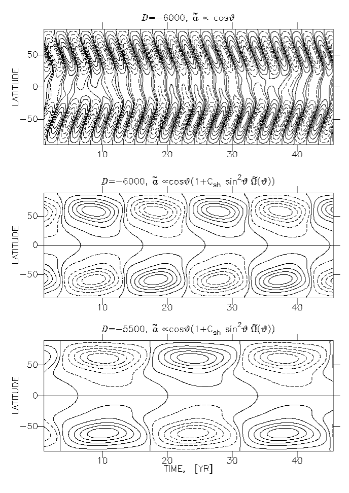
Figure 6: The butterfly diagrams of the large-scale toroidal magnetic field evolution for different type of the $\alpha$ effect distribution. Time was computed by taking $\eta_{T}=10^{13}\ cm^{2}/s$ and $R_{\odot}=6.96\cdot 10^{10}\ cm$ into account.

The critical dynamo-numbers and some results about the non-linear behavior of (42) with $\alpha\propto\cos\theta$ were considered in more detail by Kitchatinov et al.(1994) and Kitchatinov & Pipin(1998). Equations (42) give oscillatory solutions for negative dynamo numbers. The most interesting solution with long-term modulations of magnetic field and the shear was found by Kitchatinov et al.(1994) for a slightly supercritical regime, ${\cal D}=-6000$. Here we repeat these simulations for a different type of the $\alpha$ - effect.

Figure 6 shows some results of the numerical simulations. The upper panel demonstrates the long-term evolution of the butterfly diagrams of the toroidal field in coordinates time-latitude for $\alpha\propto\cos\theta$. This diagram is in agreement with the previous findings in papers by Kitchatinov et al.(1994) and Kitchatinov & Pipin(1998). The middle panel on Figure 6 shows the same for an $\alpha$ effect dependent on the shear, (43), and with the same ${\cal D}=-6000$. There are several differences between pictures. The first one is that the second case does not show the long-term oscillations despite the non-linear interplay between magnetic field and shear. Next, the butterfly wings are too concentrated near the pole. The last difference is that period of the considered dynamo is about 5 times larger. This effect is likely due to the space separation between $\alpha$ and $\Omega$ effects on latitude. Such an effect was discussed firstly by Deinzer et al. (1974). This latitude separation is also probable reason for the polar concentration of magnetic field. The down panel on Figure 6 shows the evolution of the toroidal magnetic field with the general type of $\tilde{\alpha}$, (43), and with ${\cal D}=-5500$. The period of dynamo is 8 times large there than for the ”usual” $\alpha$ effect and it is comparable with the solar cycle period.

The critical dynamo number for the dynamo with the shear-dominated $\alpha$ effect is about ${\cal D}=-5400$. We also tried to explore the limiting case where the $\alpha$ was defined only by the shear contributions, i.e, $\tilde{\alpha}$ has form like $\tilde{\alpha}\propto\cos\theta\sin^{2}\theta\tilde{\Omega}$. Only steady solutions were found for the negative dynamo numbers in this case. This issue is also in agreement with analysis in the paper by Deinzer et al. (1974), who also found the steady type solution after the space separation between $\alpha$ and $\Omega$ effects approaches to some limit.

4 Conclusions.

Let us summarize our findings. We have explored the $\alpha$ effect and the small-scale current helicity for the case of weakly compressible magnetically driven turbulence that is subjected to differential rotation. The derivations presented here were made without restriction on the angular velocity amplitude, i.e., for an arbitrary Coriolis number. The differential rotation itself assumed to be weak. The main finding is that for the fast rotation case the influence of the differential rotation on the $\alpha$ effect and $h_{c}$ can be quite strong. Both $\alpha$ and $h_{c}$ become non-monotonic functions of the latitude with two maxima in one hemisphere. One maximum is at mid latitude and another is at the pole as in standard theory.

Beneath the solar convection zone, at the northern hemisphere, $\alpha^{\phi\phi}$ is likely to have a negative sign at mid-latitudes. However, this result is not conclusive. The problem is that for the magnetically driven $\alpha$ effect the ”standard”, $\cos\theta$-like contributions quenches for the fast rotation case as $\Omega^{*\ -1}$, and the shear contributions approaches to a constant. Thus the negative sign of the $\alpha$ is the result of such a behavior of the competitive contributions. Since we know the hydrodynamic part of the $\alpha^{\phi\phi}$ approaching a constant under the fast rotating limit (Rüdiger & Kitchatinov 1993), for a more reliable estimation of the $\alpha$ effect the hydrodynamic part is should also be incorporated.

A debate is ongoing in the literature about whether the relation between $\alpha$ and $h_{c}$, which was proposed by Keinig (1983), Rädler & Seehafer (1990) and Seehafer (1994), is a fundamental one. It is a very important question because this relation can be used in solar physics as a diagnostic tool to for defining the $\alpha$ effect parameters in the Solar convection zone. The present computations show that the phase relation between the two holds (in the sense Keinigs’ formula) for the slow rotation case eqs.(26,27,36,37), sf. Rüdiger & Pipin (2000), and so does for the fast rotation case eqs. (28,29,38, 39). The Keinig-Seehafer’s formula is violated for intermediate values of $\Omega^{*}$ and shear. This is clearly seen in Figures 3 and 4. The validity of Keinig-Seehafer’s identity depends largely on the assumed stationarity and homogeneity of the turbulent flows. Such an approximation is probably valid for the slow rotation case or for the saturated state in the fast rotation limit. In addition, the phase relation can be violated due to contributions from kinetic helicity. It is known that the isotropic $\alpha$ effect can be expressed by the sum of kinetic and current helicities, e.g., Field et al (1999). Such a representation reflects the fact that $\alpha$ can be divided into the ”hydrodynamic” and ”magnetic” parts. We skip the ”hydrodynamic” part in the paper. Hence we can not make a conclusive statement about the relation $\alpha$ to $h_{c}$ in a general case.

Aplication of $\alpha^{\phi\phi}$ contributed by shear to simple 1D model shows the drastic differences in evolution of the generated large-scale magnetic field compared to the case where $\alpha^{\phi\phi}\propto\cos\theta$. The shear contributions to $\alpha^{\phi\phi}$ cause the spatial separation between $\alpha$ and $\Omega$ generation processes. As noted by Deinzer et al(1974), such a separation results to increase of the dynamo period. Our simulations show that the interface dynamo driven by shear-dominated $\alpha$ effect (and with parameters adjusted to match conditions near the bottom or right beneath the SCZ) has a period about 1 diffusion time which is comparable with the Solar cycle period. Though, the obtained butterfly diagrams are not in agreement with observations. This could be improve by including the contributions from the meridional circulation or from the anisotropic turbulent transport effects (Kitchatinov 1990). Unfortunately, at least for the solar case, the solution of the period cycle problem obtained from this 1D model can not be extended for the distributed dynamo in the spherical shell, because the radial shear is weak in the main part of convection zone and the Coriolis number is not strong enough there. This conclusion is well illustrated by Figures 2,3. As can be seen, the influence of the differential rotation on the latitudinal distribution of $\alpha$ is quite strong but not enough to be the decisive factor.

Nevertheless, in the spherical shell dynamos the contributions of the differential rotation to the $\alpha$ effect can introduce an interesting component in the non-linear feedback reaction of the magnetic field on the $\alpha$ effect. The magnetic field is well known to suppress the $\alpha$. However, the numerical simulations show the radial gradient of the angular velocity is also likely to be increased in the regions with the strong magnetic fields (cf. Pipin 1999). Then we might well expect the $\alpha$ effect contributed by shear will be less suppressed by the Lorentz forces than contributions connected with rigid rotation. This conclusion should be checked by computing the shear-dominated alpha effect after taking the influence of magnetic field on the turbulence into account. Such an argument also should be considered in numerical simulation devoted to the magnetic quenching of alpha effect (cf. Ossendrijver et al 2001).

Another interesting point which could be discussed in the light of the results obtained connects with idea that in fully developed turbulence the hydrodynamic and magnetic parts of $\alpha$ effect cancel each other, Vainshtein (1980). For the rigid rotation case, as we noted above, the magnetic part of alpha effect is quenched opposite to increase the Coriolis number. However its hydrodynamic part tends to the constant (Rüdiger & Kitchatinov 1993). Consequently, these counterparts are hardly canceled for the fast rotating system. Our paper (as well as paper of Rüdiger & Kitchatinov 1993) is based on the considering the real sources of the alpha effect in rotating stratified turbulence. This differs from publications were the hydrodynamic and magnetic helicity spectrum are defined a priori (eg. Vainshtein 1980, Field et al. 1999). In principle, an ideal choice involves computing the combination of the hydrodynamic and magnetic parts of the $\alpha$ effect while including compressibility effects equally in both the density and intensity stratifications cases and further taking into account the differential rotation, and the non-linear magnetic feedback. We hope to take some steps along this direction in future.

5 Appendix

The functions used in this paper are as follows,

$$f_{1}=-\frac{1}{{4\Omega^{*}}^{5}}\left({\Omega^{*}}\left(3+2\,{\Omega^{*}}^{2}\right)-3\left(1+{\Omega^{*}}^{2}\right)\arctan({\Omega^{*}})\right),$$

$$f_{2}=\frac{3}{64\,{\Omega^{*}}^{5}}\bigl{(}{\Omega^{*}}\left(15+{\Omega^{*}}^{2}\right)+(-15-6{\Omega^{*}}^{2}+{\Omega^{*}}^{4})\arctan({\Omega^{*}})\bigr{)},$$

$$f_{4}=\frac{1}{192{\Omega^{*}}^{9}(1+{\Omega^{*}}^{2})}\Bigl{(}{\Omega^{*}}(-2205-3360{\Omega^{*}}^{2}-876{\Omega^{*}}^{4}+384{\Omega^{*}}^{6}+73{\Omega^{*}}^{8})$$

$$+9(245+455{\Omega^{*}}^{2}+200{\Omega^{*}}^{4}-32{\Omega^{*}}^{6}-21{\Omega^{*}}^{8}+{\Omega^{*}}^{10})\arctan({\Omega^{*}})\Bigr{)},$$

$$f_{6}=\frac{1}{192{\Omega^{*}}^{9}(1+{\Omega^{*}}^{2})}\bigl{(}{\Omega^{*}}(-2205-3360{\Omega^{*}}^{2}-1011{\Omega^{*}}^{4}+240{\Omega^{*}}^{6}+64{\Omega^{*}}^{8})$$

$$-9(-245-455{\Omega^{*}}^{2}-215{\Omega^{*}}^{4}+11{\Omega^{*}}^{6}+16{\Omega^{*}}^{8})\arctan({\Omega^{*}})\bigr{)},$$

$$f_{7}=\frac{1}{960{\Omega^{*}}^{9}(1+{\Omega^{*}}^{2})}\Bigl{(}9135{\Omega^{*}}+13440{\Omega^{*}}^{3}+3307{\Omega^{*}}^{5}-2148{\Omega^{*}}^{7}-870{\Omega^{*}}^{9}$$

$$-15(609+1099{\Omega^{*}}^{2}+465{\Omega^{*}}^{4}-121{\Omega^{*}}^{6}-102{\Omega^{*}}^{8}-6{\Omega^{*}}^{10})\arctan({\Omega^{*}})\Bigr{)},$$

$$f_{8}=\frac{1}{960{\Omega^{*}}^{9}(1+{\Omega^{*}}^{2})}\Bigl{(}{\Omega^{*}}(-9135-13440{\Omega^{*}}^{2}-2002{\Omega^{*}}^{4}+4068{\Omega^{*}}^{6}$$

$$+1485{\Omega^{*}}^{8})+15(609+1099{\Omega^{*}}^{2}+378{\Omega^{*}}^{4}-278{\Omega^{*}}^{6}$$

$$-195{\Omega^{*}}^{8}-29{\Omega^{*}}^{10})\arctan({\Omega^{*}})\Bigr{)},$$

$$f_{9}=\frac{1}{960{\Omega^{*}}^{9}(1+{\Omega^{*}}^{2})}\Bigl{(}47565{\Omega^{*}}+70560{\Omega^{*}}^{3}+15133{\Omega^{*}}^{5}-12252{\Omega^{*}}^{7}$$

$$-3710{\Omega^{*}}^{9}-15(3171+5761{\Omega^{*}}^{2}+2295{\Omega^{*}}^{4}-751{\Omega^{*}}^{6}-486{\Omega^{*}}^{8}$$

$$-30{\Omega^{*}}^{10})\arctan({\Omega^{*}})\Bigr{)},$$

$$f_{11}=\frac{1}{960{\Omega^{*}}^{9}(1+{\Omega^{*}}^{2})}\Bigl{(}9135{\Omega^{*}}+13440{\Omega^{*}}^{3}+2182{\Omega^{*}}^{5}-3168{\Omega^{*}}^{7}-885{\Omega^{*}}^{9}$$

$$+15(-609-1099{\Omega^{*}}^{2}-390{\Omega^{*}}^{4}+214{\Omega^{*}}^{6}+119{\Omega^{*}}^{8}+5{\Omega^{*}}^{10})\arctan({\Omega^{*}})\Bigr{)},$$

$$f_{12}=\frac{1}{960{\Omega^{*}}^{9}(1+{\Omega^{*}}^{2})}\Bigl{(}{\Omega^{*}}(-9135-13440{\Omega^{*}}^{2}-2587{\Omega^{*}}^{4}+2688{\Omega^{*}}^{6}$$

$$+810{\Omega^{*}}^{8})-15(-609-1099{\Omega^{*}}^{2}-417{\Omega^{*}}^{4}+173{\Omega^{*}}^{6}+110{\Omega^{*}}^{8}$$

$$+10{\Omega^{*}}^{10})\arctan({\Omega^{*}})\Bigr{)},$$

$$f_{13}=\frac{1}{64{\Omega^{*}}^{5}(1+{\Omega^{*}}^{2})}\Bigl{(}{\Omega^{*}}(-135-84{\Omega^{*}}^{2}+11{\Omega^{*}}^{4})+(135+129{\Omega^{*}}^{2}+5{\Omega^{*}}^{4}$$

$$+11{\Omega^{*}}^{6})\arctan({\Omega^{*}})\Bigr{)},$$

$$f_{14}=\frac{1}{64{\Omega^{*}}^{5}(1+{\Omega^{*}}^{2})}\Bigl{(}-27{\Omega^{*}}+4{\Omega^{*}}^{3}+7{\Omega^{*}}^{5}+(27+5{\Omega^{*}}^{2}-15{\Omega^{*}}^{4}$$

$$+7{\Omega^{*}}^{6})\arctan({\Omega^{*}})\Bigr{)},$$

$$f_{15}=\frac{1}{192{\Omega^{*}}^{9}(1+{\Omega^{*}}^{2})}\Bigl{(}2205{\Omega^{*}}+3360{\Omega^{*}}^{3}+1686{\Omega^{*}}^{5}+372{\Omega^{*}}^{7}-55{\Omega^{*}}^{9}$$

$$+9(-245-455{\Omega^{*}}^{2}-290{\Omega^{*}}^{4}-82{\Omega^{*}}^{6}-{\Omega^{*}}^{8}+{\Omega^{*}}^{10})\arctan({\Omega^{*}})\Bigr{)},$$

$$f_{17}=\frac{1}{960{\Omega^{*}}^{9}(1+{\Omega^{*}}^{2})^{2}}\Bigl{(}63945{\Omega^{*}}+143325{\Omega^{*}}^{3}+80954{\Omega^{*}}^{5}-17822{\Omega^{*}}^{7}$$

$$-23331{\Omega^{*}}^{9}-3615{\Omega^{*}}^{11}+15(1+{\Omega^{*}}^{2})^{2}(-4263-2450{\Omega^{*}}^{2}$$

$$+960{\Omega^{*}}^{4}+570{\Omega^{*}}^{6}+15{\Omega^{*}}^{8})\arctan({\Omega^{*}})\Bigr{)}$$

$$f_{18}=\frac{1}{960{\Omega^{*}}^{9}(1+{\Omega^{*}}^{2})}\Bigl{(}9135{\Omega^{*}}+13440{\Omega^{*}}^{3}+2182{\Omega^{*}}^{5}-2988{\Omega^{*}}^{7}$$

$$-825{\Omega^{*}}^{9}+15(-609-1099{\Omega^{*}}^{2}-390{\Omega^{*}}^{4}+202{\Omega^{*}}^{6}+111{\Omega^{*}}^{8}$$

$$+9{\Omega^{*}}^{10})\arctan({\Omega^{*}})\Bigr{)},$$

$$f_{19}=\frac{1}{192{\Omega^{*}}^{9}(1+{\Omega^{*}}^{2})^{2}}\Bigl{(}9135{\Omega^{*}}+19635{\Omega^{*}}^{3}+10347{\Omega^{*}}^{5}-2369{\Omega^{*}}^{7}$$

$$-2634{\Omega^{*}}^{9}-354{\Omega^{*}}^{11}+15(1+{\Omega^{*}}^{2})^{2}(-609-294{\Omega^{*}}^{2}+125{\Omega^{*}}^{4}$$

$$+60{\Omega^{*}}^{6}+2{\Omega^{*}}^{8})\arctan({\Omega^{*}})\Bigr{)}$$

$$f_{20}=\frac{1}{32{\Omega^{*}}^{5}(1+{\Omega^{*}}^{2})}\Bigl{(}15{\Omega^{*}}+4{\Omega^{*}}^{3}-3{\Omega^{*}}^{5}-3(5+3{\Omega^{*}}^{2}-{\Omega^{*}}^{4}$$

$$+{\Omega^{*}}^{6})\arctan({\Omega^{*}})\Bigr{)},$$

$$f_{22}=\frac{1}{192{\Omega^{*}}^{9}(1+{\Omega^{*}}^{2})}\Bigl{(}{\Omega^{*}}(2205+3360{\Omega^{*}}^{2}+1686{\Omega^{*}}^{4}+804{\Omega^{*}}^{6}$$

$$+281{\Omega^{*}}^{8})-3(735+1365{\Omega^{*}}^{2}+870{\Omega^{*}}^{4}+390{\Omega^{*}}^{6}$$

$$+163{\Omega^{*}}^{8}+13{\Omega^{*}}^{10})\arctan({\Omega^{*}})\Bigr{)},$$

$$f_{23}=\frac{1}{192{\Omega^{*}}^{9}(1+{\Omega^{*}}^{2})}\Bigl{(}2205{\Omega^{*}}+3360{\Omega^{*}}^{3}+876{\Omega^{*}}^{5}-384{\Omega^{*}}^{7}-73{\Omega^{*}}^{9}$$

$$-9(245+455{\Omega^{*}}^{2}+200{\Omega^{*}}^{4}-32{\Omega^{*}}^{6}-21{\Omega^{*}}^{8}+{\Omega^{*}}^{10})\arctan({\Omega^{*}})\Bigr{)},$$

$$f_{25}=\frac{1}{4{\Omega^{*}}^{5}}\Bigl{(}-{\Omega^{*}}(3+2{\Omega^{*}}^{2})+3(1+{\Omega^{*}}^{2})\arctan({\Omega^{*}})\Bigr{)},$$

$$f_{27}=\frac{1}{4{\Omega^{*}}^{5}}\left(-3\,{\Omega^{*}}+\left(3+{\Omega^{*}}^{2}\right)\,\arctan({\Omega^{*}})\right),$$

$$f_{28}=\frac{1}{4{\Omega^{*}}^{5}}\left({\Omega^{*}}\,\left(15+4\,{\Omega^{*}}^{2}\right)-3\,\left(5+3\,{\Omega^{*}}^{2}\right)\,\arctan({\Omega^{*}})\right),$$

$$f_{29}=\frac{3}{64{\Omega^{*}}^{5}(1+{\Omega^{*}}^{2})}\Bigl{(}{\Omega^{*}}(75+68{\Omega^{*}}^{2}+{\Omega^{*}}^{4})$$

$$-(75+93{\Omega^{*}}^{2}+17{\Omega^{*}}^{4}-{\Omega^{*}}^{6})\arctan({\Omega^{*}})\Bigr{)}$$

$$f_{30}=\frac{1}{96{\Omega^{*}}^{9}(1+{\Omega^{*}}^{2})^{2}}\Bigl{(}15435{\Omega^{*}}+35175{\Omega^{*}}^{3}+22212{\Omega^{*}}^{5}-76{\Omega^{*}}^{7}$$

$$-2895{\Omega^{*}}^{9}-283{\Omega^{*}}^{11}-3(1+{\Omega^{*}}^{2})^{2}(5145+3150{\Omega^{*}}^{2}-590{\Omega^{*}}^{4}$$

$$-330{\Omega^{*}}^{6}+9{\Omega^{*}}^{8})\arctan({\Omega^{*}})\Bigr{)},$$

$$f_{31}=\frac{3}{64{\Omega^{*}}^{5}(1+{\Omega^{*}}^{2})}\Bigl{(}{\Omega^{*}}(105+100{\Omega^{*}}^{2}+3{\Omega^{*}}^{4})+3(-35-45{\Omega^{*}}^{2}$$

$$-9{\Omega^{*}}^{4}+{\Omega^{*}}^{6})\arctan({\Omega^{*}})\Bigr{)},$$

$$f_{32}=\frac{1}{32{\Omega^{*}}^{5}}\bigl{(}3{\Omega^{*}}(-1+{\Omega^{*}}^{2})+(3-2{\Omega^{*}}^{2}+3{\Omega^{*}}^{4})\arctan({\Omega^{*}})\bigr{)},$$

$$f_{\alpha 1}=\frac{1}{160{\Omega^{*}}^{8}(1+{\Omega^{*}}^{2})}\Bigl{(}10080{\Omega^{*}}+15120{\Omega^{*}}^{3}+3431{\Omega^{*}}^{5}-2324{\Omega^{*}}^{7}-595{\Omega^{*}}^{9}$$

$$+15(-672-1232{\Omega^{*}}^{2}-505{\Omega^{*}}^{4}+137{\Omega^{*}}^{6}+85{\Omega^{*}}^{8}+3{\Omega^{*}}^{10})\arctan({\Omega^{*}})\Bigr{)},$$

$$f_{\alpha 2}=-\frac{1}{32\,{\Omega^{*}}^{4}}\left({\Omega^{*}}\,\left(111+25\,{\Omega^{*}}^{2}\right)-\left(111+62\,{\Omega^{*}}^{2}+7\,{\Omega^{*}}^{4}\right)\,\arctan({\Omega^{*}})\right),$$

$f_{3,5,10,21}=-f_{2},f_{16}=f_{4},f_{24}=-\frac{3}{2}f_{20},f_{26}=f_{2},f_{33}=-f_{11}$. The current helicity was defined with the following functions,

$$\psi_{0}=\frac{6\,{\Omega^{*}}+4\,{\Omega^{*}}^{3}-6\,\left(1+{\Omega^{*}}^{2}\right)\,\arctan({\Omega^{*}})}{4{\Omega^{*}}^{5}},$$

$$\psi_{1}=\frac{-\left({\Omega^{*}}\,\left(33+58\,{\Omega^{*}}^{2}+29\,{\Omega^{*}}^{4}\right)\right)+3\,{\left(1+{\Omega^{*}}^{2}\right)}^{2}\,\left(11+{\Omega^{*}}^{2}\right)\,\arctan({\Omega^{*}})}{48\,{\Omega^{*}}^{5}\,\left(1+{\Omega^{*}}^{2}\right)},$$

$$\psi_{2}=\frac{}{96\,{\Omega^{*}}^{5}(1+{\Omega^{*}}^{2})}\Bigl{(}{\Omega^{*}}\,\left(-645-532\,{\Omega^{*}}^{2}+9\,{\Omega^{*}}^{4}\right)$$

$$+3\,\left(215+249\,{\Omega^{*}}^{2}+37\,{\Omega^{*}}^{4}+3\,{\Omega^{*}}^{6}\right)\,\arctan({\Omega^{*}})\Bigr{)}$$

$$\psi_{3}=\frac{1}{96{\Omega^{*}}^{5}(1+{\Omega^{*}}^{2})}\Bigl{(}{\Omega^{*}}(75+144{\Omega^{*}}+92{\Omega^{*}}^{2}+240{\Omega^{*}}^{3}+9{\Omega^{*}}^{4}+96{\Omega^{*}}^{5})$$

$$+3(-25-48{\Omega^{*}}-39{\Omega^{*}}^{2}-96{\Omega^{*}}^{3}-11{\Omega^{*}}^{4}-48{\Omega^{*}}^{5}+3{\Omega^{*}}^{6})\arctan({\Omega^{*}})\Bigr{)},$$

$$\psi_{4}=\frac{-6\,{\Omega^{*}}+2\,\left(3+{\Omega^{*}}^{2}\right)\,\arctan({\Omega^{*}})}{4{\Omega^{*}}^{5}},$$

$$\psi_{5}=\frac{2\,{\Omega^{*}}\,\left(15+{\Omega^{*}}^{2}-8\,{\Omega^{*}}^{4}\right)+6\,\left(-5-2\,{\Omega^{*}}^{2}+3\,{\Omega^{*}}^{4}\right)\,\arctan({\Omega^{*}})}{12\,{\Omega^{*}}^{5}\,\left(1+{\Omega^{*}}^{2}\right)},$$

$$\psi_{6}=\frac{{\Omega^{*}}\,\left(27+54\,{\Omega^{*}}^{2}+23\,{\Omega^{*}}^{4}\right)-9\,{\left(1+{\Omega^{*}}^{2}\right)}^{2}\,\left(3+{\Omega^{*}}^{2}\right)\,\arctan({\Omega^{*}})}{24\,{\Omega^{*}}^{5}\,\left(1+{\Omega^{*}}^{2}\right)},$$

$$\psi_{7}\frac{{\Omega^{*}}\,\left(-15-4\,{\Omega^{*}}^{2}+3\,{\Omega^{*}}^{4}\right)+3\,\left(5+3\,{\Omega^{*}}^{2}-{\Omega^{*}}^{4}+{\Omega^{*}}^{6}\right)\,\arctan({\Omega^{*}})}{48\,{\Omega^{*}}^{5}\,\left(1+{\Omega^{*}}^{2}\right)},$$

$$\psi_{8}=\frac{{\Omega^{*}}\,\left(3+2\,{\Omega^{*}}^{2}+3\,{\Omega^{*}}^{4}\right)+3\,\left(-1+{\Omega^{*}}^{2}\right)\,{\left(1+{\Omega^{*}}^{2}\right)}^{2}\,\arctan({\Omega^{*}})}{24\,{\Omega^{*}}^{4}\,\left(1+{\Omega^{*}}^{2}\right)},$$

$$\psi_{9}=\frac{{\Omega^{*}}\,\left(15+13\,{\Omega^{*}}^{2}\right)-3\,\left(5+6\,{\Omega^{*}}^{2}+{\Omega^{*}}^{4}\right)\arctan({\Omega^{*}})}{24\,{\Omega^{*}}^{5}},$$

$$\psi_{10}=\frac{{\Omega^{*}}\,\left(-9+{\Omega^{*}}^{2}\right)+\left(9+2\,{\Omega^{*}}^{2}+{\Omega^{*}}^{4}\right)\,\arctan({\Omega^{*}})}{16\,{\Omega^{*}}^{4}},$$

$$\psi_{h1}=\frac{1}{96{\Omega^{*}}^{4}(1+{\Omega^{*}}^{2})}\Bigl{(}{\Omega^{*}}(-405-228{\Omega^{*}}^{2}+73{\Omega^{*}}^{4})$$

$$+3(135+121{\Omega^{*}}^{2}-11{\Omega^{*}}^{4}+3{\Omega^{*}}^{6})\arctan({\Omega^{*}})\Bigr{)},$$

$$\psi_{h2}=\frac{1}{96\,{\Omega^{*}}^{4}\,\left(1+{\Omega^{*}}^{2}\right)}\Bigl{(}{\Omega^{*}}\,\left(117+192\,{\Omega^{*}}^{2}+43\,{\Omega^{*}}^{4}\right)$$

$$-3\,\left(39+77\,{\Omega^{*}}^{2}+45\,{\Omega^{*}}^{4}+7\,{\Omega^{*}}^{6}\right)\,\arctan({\Omega^{*}})\Bigr{)}$$

References

- [1] [] Balbus, S.A.& Hawley, J.F., ”A powerful local shear instability in weakly magnetized disks”, ApJ, 376, 214B (1991)
- [2] [] Belvedere, G, Kuzanyan, K.M., & Sokoloff, D.D.,”A two-dimensional asymptotic solution for a dynamo wave in the light of the solar internal rotation”, MNRAS, 315, 778 (2000).
- [3] [] Biskamp, D. , ”Nonlinear Magnetohydrodynamics”, Cambridge University Press (1997).
- [4] [] Blackman, E, ”Mean magnetic field generation in sheared rotators”, ApJ, 529, 138 (2000).
- [5] [] Brandenburg, A., in Advances in Solar Physics, ed. G. Belvedere, W.Mattig, & M.Rodonó, Lect. Notes Phys., 432, Springer-Verlag, (1994).
- [6] [] Brandenburg, A., ”The inverse cascade and non-linear alpha-effect in simulations of isotropic helical hydromagnetic turbulence”, ApJ, 550, 824 (2001).
- [7] [] Brandenburg, A., ”Simulations and Observations of Stellar Dynamos: Evidence for a Magnetic Alpha-Effect”, in ”Stellar Dynamos: Nonlinearity and Chaotic Flows”, ASP Conference Series 178, ed. Manuel Nunez and Antonio Ferriz-Mas., 13 (1999).
- [8] [] Cattaneo, F., & Hughes, D.W., ”Nonlinear saturation of the turbulent alpha effect”, Phys. Rev. E., 54, 4532 (1996).
- [9] [] Field, G.B., Blackman, E.G., & Chou, H., ”Nonlinear -effect in dynamo theory.”, ApJ, 513, 638 (1999).
- [10] [] Frish, U. Pouquet, A., Léorat, I., Mazure, A., J. , ”Possibility of an inverse cascade of magnetic helicity in magnetohydrodynamic turbulence”, Fluid Mech., 1975, 68, 4, 769.
- [11] [] Kitchatinov, L.L., ”Turbulent transport of magnetic fields in a highly conducting rotating fluid and the solar cycle”, A&A, 243, 483 (1991).
- [12] [] Kitchatinov, L. L., Mazur, M. V., Jardine, M., ”Magnetic field escape from a stellar convection zone and the dynamo-cycle period”, A&A, 359, 531(2000).
- [13] [] Kitchatinov, L.L., & Pipin V.V., ”Mean field buoyancy”, A&A, 274,674 (1993).
- [14] [] Kosovichev, A.G., Schou J. et al., ”Structure and rotation of the Solar interior: initial results from the MDI medium-L Progra”, Solar Phys., 170,43(1997).
- [15] [] Krause, F. & Rädler, K.-H., ”Mean Field Magnetohydrodynamics and Dynamo Theory”, Oxford, Pergamon Press(1980).
- [16] [] Kuzanyan, K., Bao, S., & Zhang, H., ”Probing signatures of the alpha-effect in the solar convection zone”, Solar Phys., 191, 231 (2000).
- [17] [] Moffatt, H.K., ”Magnetic Field Generation in Electrically Conducting Fluids, Cambridge Univ. Press, (1978)
- [18] [] Moffatt, H.K., ”Reflections on magnetohydrodynamics” in ”Perspectives in Fluid Dynamics”, eds. G.K.Batchelor, H.K. Moffatt, M.G. Worster, Cambridge Univ. Press, 347 (2000).
- [19] [] Ossendrijver M., Stix, M., & Brandenburg A., ”Magnetoconvection and dynamo coefficients: Dependence of the effect on rotation and magnetic field.”, A&A, 376, 713 (2001).
- [20] [] Parker, E.N., ”Cosmical Magnetic Fields”, Oxford, Clarendon Press (1979).
- [21] [] Parker, E.N., ”A solar dynamo surface wave at the interface between convection and nonuniform rotation”, ApJ, 408, 707 (1993).
- [22] [] Pevtsov, A.A., Canfield, R.C., & Metcalf, T.R.,”Latitudinal variation of helicity of photospheric magnetic fields”, ApJ, 440L, 109(1995).
- [23] [] Pope, S.B.,”Stochastic Lagrangian models for turbulence,” Ann.Rev.Fluid Mech., 26, 23 (1994) .
- [24] [] Pouquet, A., Frisch, U., Leorat, J., ”Strong MHD helical turbulence and the nonlinear dynamo effect”, J.Fluid Mech., 77(2),321 (1976).
- [25] [] Rüdiger,G., & Kitchatinov, L.L., ”Alpha-effect and alpha-quenching”, A&A, 269, 581 (1993).
- [26] [] Rüdiger,G., & Pipin, V.V., ”Viscosity-alpha and dynamo-alpha for magnetically driven compressible turbulence in Kepler disks.”, A&A, 362, 756 (2000).
- [27] [] Rüdiger,G., Pipin, V.V., & Belvedere G., ”Alpha-effect, helicity and angular momentum transport for a magnetically driven turbulence in the solar convection zone”, Solar Phys., 198, 241 (2001).
- [28] [] Seehafer, N., ”Electric current helicity in the solar atmosphere”, Solar Phys., 125, 219 (1990).
- [29] [] Seehafer, N., Europhys. Lett., 27,353 (1994)
- [30] [] Vainshtein, S.I., & Cattaneo, F., ”Nonlinear restrictions on dynamo action”, ApJ, 393, 165 (1992).
- [31] [] Vainshtein, S.I., ”The Cosmic Magnetic Fields”, Moskow, Nauka (1980).