The Star Formation Rate-Density Relationship at Redshift 3

Abstract

We study the star formation rate (SFR) as a function of environment for UV-selected Lyman break galaxies (LBGs) at redshift 3. From deep ($\mu_{I,\rm AB}(sky)\simeq 27.6$) $UBVI$ KPNO 4-m/MOSAIC images, covering a total of 0.90 deg², we select 334 LBGs in slices $100$$h^{-1}$ Mpc (co-moving) deep spanning the redshift range $2.9<z<3.4$ based on Bayesian photometric redshifts that include the $I$ magnitude as a prior. The slice width ($100$$h^{-1}$ Mpc) corresponds to the photometric redshift accuracy ($\Delta_{z}\sim 0.15$). We used mock catalogs from the GIF2 cosmological simulations to show that this redshift resolution is sufficient to statistically differentiate the high-density regions from the low-density regions using $\Sigma_{5}$, the projected density to the fifth nearest neighbor. These mock catalogs have a redshift depth of $110$$h^{-1}$ Mpc, similar to our slice width. The large area of the MOSAIC images, $\sim 40\times 40$ Mpc (co-moving) per field, allows us to measure the SFR from the dust-corrected UV continuum as a function of $\Sigma_{5}$. In contrast to low-redshift galaxies, we find that the SFR (or UV luminosity) of LBGs at $z=3$ shows no detectable dependence on environment over 2 orders of magnitude in density. To test the significance of our result, we use Monte Carlo simulations (from the mock catalogs) and the same projected density estimators that we applied to our data. We find that we can reject the steep $z=0$ SFR-density relation at the 5$-\sigma$ level. We conclude that the SFR-density relation at $z=3$ must be at least 3.6 times flatter than it is locally, i.e. the SFR of LBGs is significantly less dependent on environment than the SFR of local star-forming galaxies. We find that the rest-frame UV colors are also independent of environment.

1 Introduction

There is a long history of results showing that galaxy properties vary as a function of environments such as the morphology-density relation in clusters (Melnick & Sargent, 1977; Dressler, 1980; Postman & Geller, 1984; Dressler et al., 1997; Treu et al., 2003) and its associated star formation rate-density relation (e.g., Lewis et al., 2002). Lewis et al. (2002) used the Two-Degree Field Galaxy Redshift Survey (2dFGRS; Colless et al., 2001) to show that the anti-correlation between star formation rate (SFR) and local projected density holds in clusters up to 2 virial radii from the cluster center. Not only is the mean luminosity a function of environment (Blanton et al., 2003; Hogg et al., 2003; Balogh et al., 2004), but the luminosity function (LF) is also a continuous function of the local density (e.g. Croton et al., 2004).

The SFR also depends on the local density in groups and in the field. Gómez et al. (2003) showed similar results using the Early Data Release (Stoughton & et al.,, 2002) of the Sloan Digital Sky Survey (SDSS), and they also showed that the SFR-density relation holds for field galaxies. Balogh et al. (2004) used both the 2dFGRS and the SDSS to show that the SFR (as measured by the H$\alpha$ equivalent width) of field galaxies is strongly dependent on the local projected density. All these results point to the existence of physical mechanisms that quench star formation as the local density increases, from the field to groups to clusters.

At $z=0.4$, the quenching of star-formation is apparently already in place. Using the wide-field ($\sim 30$′) imager SuprimeCam at the Subaru 8-m telescope, Kodama et al. (2001) selected members of the $z=0.41$ cluster A851 using photometric redshifts and found that the colors of faint galaxies are strongly dependent on the local galaxy density. Follow-up narrow band H$\alpha$ imaging of this cluster showed that the fraction of star-forming galaxies is a strong function of the local projected density far ($\gtrsim$1$h^{-1}$ Mpc) from the cluster center (Kodama et al., 2004).

No observations of the SFR-density relation have yet been made at redshifts greater than one. Here, we used ground-based data from the Kitt Peak 4–m telescope fitted with the MOSAIC wide-field imager to investigate whether or not the SFR-density relation already existed at redshift $z=3$. We use photometric redshifts that are accurate to $\delta_{z}\sim 0.15$ or $\sim 100~{}h^{-1}$ Mpc, comparable in co-moving distance to those of the COMBO-17 survey.

We present our data and briefly discuss our selection of Lyman break galaxies (LBGs) in section 2. We then use mock catalogs from the GIF2 collaboration (Gao et al., 2004) to show in section 3 that our photometric redshift accuracy is sufficient to statistically distinguish between low and high density regions. We estimated the SFR as in section 4. Finally, our results are presented in section 5 and conclusions in section 6.

Throughout this Letter, we adopt $\Omega_{M}=0.3$, $\Omega_{\Lambda}=0.7$ and $H_{0}=100~{}h$ km s^-1 Mpc^-1. At redshift $z\sim 3$, $H(z)\sim 4.46H_{0}$, so $\delta z=0.1$ corresponds to $67~{}h^{-1}$ Mpc in co-moving coordinates.

2 Data

The observations used here are described in detail in Bouché (2003) and Bouché & Lowenthal (2004, hereafter BL04). Briefly, we used the wide-field MOSAIC camera (Jacoby et al., 1998) at the Kitt Peak National Observatory 4m telescope to image three fields in $UBVI$ to a limiting magnitude $\mu_{I,\rm AB}(sky)\simeq 27.6$. These fields were selected for the presence of a damped Ly$\alpha$ absorber (DLA) at $z\sim 3$ in our original DLA survey (Bouché & Lowenthal, 2003, BL04). Given the camera’s field of view of 36′$\times$36′(or $\sim 40~{}h^{-1}$ Mpc on a side), our survey covers a total of 0.90 deg². We selected $\sim$3,000 LBGs within the redshift range $2.8<z_{\rm phot}<3.5$. From Monte Carlo simulations, our 50% completeness level is $I_{\rm AB}=24.8$ (${\mathcal{R}}\simeq 25$), corresponding to $\sim 0.7L^{*}$, using $L^{*}(z=3)$ from Steidel et al. (1999).

Photometric redshifts were obtained from the algorithm Hyperz (Bolzonella et al., 2000) coupled with the prior likelihood distribution given by the magnitude $m_{I}$ of each galaxy (as in Benítez, 2000). See Bouché (2003) and BL04 for a detailed description of the tests we performed on the algorithm using spectroscopic redshifts in the Hubble Deep Field-North. Up to $z<6$, the overall rms $\Delta_{z}$ is $0.1$–$0.15$, corresponding to $\sim 67$–$100$ $h^{-1}$ Mpc, and $\Delta_{z}/(1+z_{\rm spec})$ is $0.06$.

In order to selected LBGs in a narrow redshift slice, we used the criterion:

$$P(z_{\rm 0}\pm W_{z}/2)>0.5,$$ (1)

where $z_{0}$ is the slice redshift, $W_{z}$ is the redshift slice width, and $P(z)$ is the redshift probability distribution (BL04). We choose a redshift width of $W_{z}=0.15$ because, as discussed in Bouché & Lowenthal (2003), it produces the largest sample in the smallest redshift slice, given the rms of the photo-$z$’s. At $z_{\rm 0}=3$, there are 68, 162, and 104 galaxies in our three fields for a total of 334.

3 Can we use photometric redshifts to measure $\Sigma_{5}$?

Before investigating the galaxy properties as a function of environment, we used the GIF2 numerical simulations of galaxy formation (described in Gao et al. 2004 and De Lucia, Kauffmann, & White 2004) to investigate whether or not, with such a coarse redshift resolution, one can make reliable density estimations based on projected surface densities. These $N$-body simulations were run with 400³ particles (each $1.73\times 10^{9}$$M_{\odot}$) over a periodic cube of 110 $h^{-1}$ Mpc on a side in a $\Lambda$ dominated universe. From the output at $z=3$ containing $\sim 29,000$ galaxies, we simulated an LBG sample by selecting 975 objects with $m_{\rm I}<25$ and $(B-V)<0.2$, where $m_{\rm I}$ is the observed $I$ magnitude given the absolute magnitude $M_{I}$, the redshift of the simulation $z=3$, and the $K$-correction according to the type of spectral energy distribution of the galaxy.

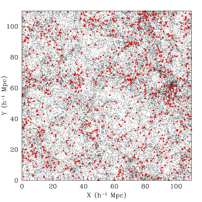
Figure 1: The $X$–$Y$ distribution (dots) of 50% (randomly selected) of the simulated galaxies of the GIF2 simulations (Gao et al., 2004). The filled triangles show all the simulated LBGs. Features of large-scale structure are visible in the simulated LBG population, considering that the galaxy positions are projected along the $z$-direction over $\sim 100h^{-1}$ Mpc. This is quantified in Fig 2.

Fig. 1 shows the two-dimensional distribution (projected along the $z$-axis) of simulated LBGs (filled triangles) along with all the galaxies (points) in the simulated GIF2 volume. One sees that the simulated LBGs do trace the major over-dense regions and filaments. Importantly, this ‘slice’ width corresponds to our redshift resolution, i.e. $\sim 100$ $h^{-1}$ Mpc.

Fig. 2 shows, for the GIF2 simulation, the two-dimensional surface density, $\Sigma_{5}$, versus the three-dimensional true density $\rho_{5}$. Both $\Sigma_{5}$ and $\rho_{5}$ are computed from the distance to the fifth nearest neighbor. The horizontal error bars reflect the $1\sigma$ rms to the mean. One order of magnitude change in $\Sigma_{n}$ corresponds to about $1.5$ orders of magnitude in $\rho_{n}$. Thus, we conclude that the projected density gives a statistical measure of the true three-dimensional over-density even when it is projected over 110 $h^{-1}$ Mpc.

4 Estimating Star Formation Rates

As reviewed by Kennicutt (1998), one can estimate the SFR from the rest–frame UV luminosity density $L_{\nu}$ in the range $1500$–$2500$ Å:

$${\rm SFR}(\hbox{$M_{\odot}$~{}yr${}^{-1}$})=1.4\times 10^{-28}L_{\nu}(\hbox{ergs s${}^{-1}$ Hz${}^{-1}$})$$ (2)

for a Salpeter initial mass function, covering the range 0.1–100 $M_{\odot}$. This relation applies only to galaxies with continuous star formation over time scales of $10^{8}$ yr or longer. Pettini et al. (2001) have shown that for a small sample of LBGs, estimates of SFR from Eq. 2 are consistent with the SFR inferred from H$\beta$ line fluxes.

We estimated the rest–frame luminosity densities (in ergs s^-1 Hz^-1) of the 334 LBGs in our MOSAIC images from the standard expression $f_{\nu}=10^{0.4\cdot(m_{\rm AB}+48.6)}/(1+z_{\rm phot})$ and from the luminosity distance. The luminosity was corrected for dust extinction. The amount of dust extinction ($A_{V}$) is estimated simultaneously with the estimation of the photometric redshift $z_{\rm phot}$. However, we found, using mock catalogs, that $A_{V}$ recovered by Hyperz is biased: $A_{V}(\hbox{true})=0.51\;A_{V}+0.32\,.$ These mock catalogs were created from the same galaxy templates, with the same extinction law used in the redshift fitting and restricted to our redshift range of interest $2.85<z<3.25$.

We used the $I$-band ($\lambda_{\rm c}=8214$ Å) flux to estimate the SFR; this filter corresponds to a rest-frame wavelength of 2000 Å for $z=3$ galaxies. We used the Calzetti et al. (2000) extinction curve  to estimate $A_{2000\AA}$, and the dust corrected SFR ($\rm SFR_{0}$) follows from $L_{\rm\nu,o}=L_{\rm\nu}10^{0.4\cdot A_{\nu}}$ and Eq. 2.

5 Results and Discussions

For galaxies at $z_{\rm phot}=3\pm 0.075$ selected with Eq. 1, Fig. 3 shows the dust-corrected star formation rate (SFR₀) as a function of the normalized local density $\Sigma_{5}/<\Sigma_{5}>$ where $\Sigma_{5}$ is the surface density within the 5th nearest neighbor, i.e. $\Sigma_{5}=6/(\pi r_{5}^{2})$, and $<\Sigma_{5}>$ is its median in each of our three MOSAIC fields. The local over-density $\delta_{5}$ is $\Sigma_{5}/<\Sigma_{5}>-1$. We use the normalized density in order to combine our several fields given that they do not contain the same mean number of LBGs per unit area. Error bars are shown for 20 randomly selected galaxies. There is no detectable difference between the distribution of SFRs of LBGs in low-density environments and those in high-density environments.

We used the Kolmogorov-Smirnov (KS) test to determine whether or not the galaxies in high density regions with $\delta_{5}>x$ are a random subset of those at $\delta_{5}<0$, i.e. they have the same SFR distribution. The top panel of Fig. 3 shows that we cannot reject the null hypothesis: the sample with $\delta_{5}<0$ and the sample with $\delta_{5}>0$ are indistinguishable. Similarly, a Pearson correlation test gives a $P$-value of $0.67$. In other words, there could be a correlation only at the 32% confidence level. We repeated the analysis for higher redshift slices, ($z_{\rm 0}=3.1$, 3.2, and 3.3) and find similar results.

Using the GIF2 simulations of section 3, we performed Monte-Carlo simulations to test whether or not the scatter in the $\Sigma_{5}$–$\rho_{5}$ relation is responsible for our null-result. We selected randomly about a third of the simulated LBGs to match our sample size of 334 LBGs. These simulated LBGs were assigned a SFR using SFR${}_{\rm sim}=(\rho_{5}/<\rho_{5}>)^{s}<{\rm SFR}>$, where $\rho_{5}$ is the same as in Fig. 2, $s$ is the slope of the simulated SFR-density relation, and $<{\rm SFR}>$ is the observed mean SFR in our data. Noise with the same properties as in the data (i.e. $\sigma(\rm{SFR})\propto$SFR) was added to SFR_sim. Note that these mock catalogs have the scatter between $\Sigma_{5}$ and $\rho_{5}$ (Fig. 2) built in. We repeated our analysis of SFR_sim versus $\Sigma_{5}$ 1000 times for values of $s$ spanning $[-0.5,0.1]$.

At $z=0$, the SFR decreases by a factor of 5 over 2 decade in density (Gómez et al., 2003; Balogh et al., 2004), i.e. $s\simeq\log(1/5)/2\simeq-0.35$. In this case, the Pearson correlation test gives a probability smaller than $10^{-6}$ (or $\sim 5$-$\sigma$) of finding no correlation. Even if we artificially increase the noise by a factor as large as 2.5, as if we had underestimated our errors by such a factor, we find that there is less than a 0.1% chance of finding no correlation if the $z=3$ SFR-density relation were as steep as at $z=0$. If the $z=3$ SFR-density relation were not as steep, but were 3.6 times flatter ($s=-0.07$), we would still have detected a correlation at the 2-$\sigma$ level.

As advocated by Hogg et al. (2003), because the local density has a signal-to-noise ratio much lower than the other physical quantities, it may be preferable to compute the mean density at constant galaxy properties (e.g., SFR, $M$, color, etc.). The left panel of Fig. 4 shows the over-density $\delta_{5}$ as a function of SFR. The running median and the 1-$\sigma$ spread are shown by the thick line and the error bars, respectively. Again, this plot reveals no evidence of an SFR-density relation.

We also investigate the dependence of galaxy color on density. The right panel of Fig. 4 shows the over-density $\delta_{5}$ as a function of the observed-frame $V-I$. Again, the running median and the 1-$\sigma$ spread are shown. The rest-frame UV colors of LBGs do not appear to change with environment. We note that this non dependence of rest-frame UV color for blue galaxies such as LBGs is similar to the results of $z=0$ surveys: in contrast to galaxies on the red sequence (e.g. Bell et al., 2004), the mean color of blue galaxies is only weakly dependent on environment (Blanton et al., 2003; Hogg et al., 2003, 2004; Balogh et al., 2004). However, we cannot rule out an environment dependence of the mean rest-frame optical colors (or age) of LBGs given that we sample only $\lambda_{\rm rest}\lesssim 2000$Å. Future rest-frame optical observations should address possible variations of the rest-frame optical colors of LBGs with environment.

6 Summary and Conclusions

From our wide-field images, covering a total of 0.90 deg², we selected $z\simeq 3$ LBGs in several redshift slices $100h^{-1}$ Mpc (co-moving) deep spanning the redshift range $2.9<z<3.4$. We computed the SFR from the UV luminosity at rest wavelength $2000$ Å. Using mock catalogs from the GIF2 simulations, we show that our photometric redshift accuracy is sufficient to statistically distinguish between low- and high-density regions using projected density estimators such as the density within the fifth nearest neighbor $\Sigma_{5}$. Our main results are as follows: we find that (1) there is no evidence of an SFR-density relation at $z=3$, and (2) the rest-frame UV colors of LBGs do not appear to change with environment.

Using Monte-Carlo simulations and the same projected density estimators that we applied to our data, we find a probability smaller than $10^{-6}$ of finding no correlation if the steep $z=0$ SFR-density relation were present in our data. If the $z=3$ SFR-density relation were about four times flatter than the $z=0$ relation, we would still have detected a correlation at the 2-$\sigma$ level. We conclude that, unless the $z=3$ SFR-density relation is even flatter, we would have detected it in our data. This is in sharp contrast to surveys at $z=0$ and $z\sim 0.4$ that have shown that the mean SFR is strongly dependent on the local galaxy density (e.g., Lewis et al., 2002; Gómez et al., 2003; Balogh et al., 2004; Kodama et al., 2004).

Very few predictions have been made of how the SFR-density relation should evolve from $z\simeq 3$ to the present. Recently, Kereš et al. (2004), using smooth particle hydrodynamic cosmological simulations, showed that the SFR-density relation is expected to be present as early as $z\sim 2$, but not at $z\sim 3$ (see their Fig. 13). See Kereš et al. (2004) and Birnboim & Dekel (2003) for a detailed description of the physical mechanisms at play. Our observed non-dependence of SFR on environment supports the theoretical results of Kereš et al. (2004).

Naturally, our sample is not representative of the entire galaxy population at $z=3$; it is biased towards blue star-forming galaxies and does not include the red population unveiled by the Faint Infrared Extragalactic Survey (Labbé et al., 2003). With the present data, we are unable to rule out the existence of a SFR-density relation if one were to include this redder population.

Figure 2: For simulated LBGs in the GIF2 simulation, the projected two-dimensional density $\Sigma_{5}$ is plotted as a function of the three-dimensional density $\rho_{5}$. Both $\Sigma_{5}$ and $\rho_{5}$ are computed from the fifth nearest neighbor. The points with error bars show the mean $\rho_{5}$ and its spread (rms) in bins of $\Sigma_{5}$. This shows that, even over 110 $h^{-1}$ Mpc, one can discriminate statistically between low- and high-density regions using projected density estimators such as $\Sigma_{5}$.

Figure 3: Bottom: For LBGs selected to be at $z_{\rm phot}=3.0\pm 0.075$ (see text), we plot the dust-corrected SFR₀ against the over-density $\delta_{5}$ obtained from $\Sigma_{5}$, the surface density within the fifth nearest neighbor. Error bars on SFR are shown for 20 (randomly selected) LBGs. Top: Results for the KS-test. For a given over-density $\delta_{5}$, the probability that the distribution of galaxies with over-densities $>\delta_{5}$ is drawn from the reference distribution (defined as $\delta_{5}<0$, left of the vertical dashed line) is shown. The distribution in the high density bins is statistically the same as in the low density bins (the 95% rejection level is indicated by the dotted line).

Figure 4: Left: The density-SFR relation at $z=3$. The filled circles show the median over-density $\delta_{5}$ in bins of SFR₀ (bin size shown by the horizontal error bar). Right: Density-color relation at $z=3$. The filled circles show the median over-density $\delta_{5}$ in color bins (bin size shown by the horizontal error bar). In both panels, the thick line shows the running median, and the vertical error bars the 1-$\sigma$ spread, respectively. The colors and SFR of LBGs are independent of the density of the surrounding galaxy.

References

- Balogh et al. (2004) Balogh, M. et al. 2004, MNRAS, 348, 1355
- Balogh et al. (2004) Balogh, M. L., Baldry, I. K., Nichol, R., Miller, C., Bower, R., & Glazebrook, K. 2004, ApJ, 615, L101
- Bell et al. (2004) Bell, E. F. et al. 2004, ApJ, 608, 752
- Benítez (2000) Benítez, N. 2000, ApJ, 536, 571
- Birnboim & Dekel (2003) Birnboim, Y., & Dekel, A. 2003, MNRAS, 345, 349
- Blanton et al. (2003) Blanton, M. R. et al. 2003, ApJ, 594, 186
- Bolzonella et al. (2000) Bolzonella, M., Miralles, J.-M., & Pelló, R. 2000, A&A, 363, 476
- Bouché (2003) Bouché, N. 2003, PhD thesis, Univ. Massachusetts, Amherst
- Bouché & Lowenthal (2003) Bouché, N., & Lowenthal, J. D. 2003, ApJ, 596, 810
- Bouché & Lowenthal (2004) —. 2004, ApJ, 609, 513
- Calzetti et al. (2000) Calzetti, D., Armus, L., Bohlin, R. C., Kinney, A. L., Koornneef, J., & Storchi-Bergmann, T. 2000, ApJ, 533, 682
- Colless et al. (2001) Colless, M. et al. 2001, MNRAS, 328, 1039
- Croton et al. (2004) Croton, J. D. et al. 2005, MNRAS, 356, 1155
- De Lucia et al. (2004) De Lucia, G., Kauffmann, G., & White, S. D. M. 2004, MNRAS, 349, 1101
- Dressler (1980) Dressler, A. 1980, ApJ, 236, 351
- Dressler et al. (1997) Dressler, A. et al. 1997, ApJ, 490, 577
- Gómez et al. (2003) Gómez, P. L. et al. 2003, ApJ, 584, 210
- Gao et al. (2004) Gao, L., White, S. D. M., Jenkins, A., Stoehr, F., & Springel, V. 2004, MNRAS, 355, 819
- Hogg et al. (2004) Hogg, D. W. et al. 2004, ApJ, 601, L29
- Hogg et al. (2003) —. 2003, ApJ, 585, L5
- Jacoby et al. (1998) Jacoby, G. H., Liang, M., Vaughnn, D., Reed, R., & Armandroff, T. 1998, in Proc. SPIE Vol. 3355, p. 721-734, Optical Astronomical Instrumentation, Sandro D’Odorico; Ed., 721–734
- Kennicutt (1998) Kennicutt, R. C. 1998, ARA&A, 36, 189
- Kereš et al. (2004) Kereš, D., Katz, N., Weinberg, D. H., & Davé, R. 2004, MNRAS, submitted, preprint (astro-ph/0407095)
- Kodama et al. (2004) Kodama, T., Balogh, M. L., Smail, I., Bower, R. G., & Nakata, F. 2004, MNRAS, 388
- Kodama et al. (2001) Kodama, T., Smail, I., Nakata, F., Okamura, S., & Bower, R. G. 2001, ApJ, 562, L9
- Labbé et al. (2003) Labbé, I. et al. 2003, AJ, 125, 1107
- Lewis et al. (2002) Lewis, I. et al. 2002, MNRAS, 334, 673
- Melnick & Sargent (1977) Melnick, J., & Sargent, W. L. W. 1977, ApJ, 215, 401
- Pettini et al. (2001) Pettini, M., Shapley, A. E., Steidel, C. C., Cuby, J., Dickinson, M., Moorwood, A. F. M., Adelberger, K. L., & Giavalisco, M. 2001, ApJ, 554, 981
- Postman & Geller (1984) Postman, M., & Geller, M. J. 1984, ApJ, 281, 95
- Steidel et al. (1999) Steidel, C. C., Adelberger, K. L., Giavalisco, M., Dickinson, M., & Pettini, M. 1999, ApJ, 519, 1
- Stoughton & et al., (2002) Stoughton, C., & et al.,. 2002, AJ, 123, 485
- Treu et al. (2003) Treu, T., Ellis, R. S., Kneib, J., Dressler, A., Smail, I., Czoske, O., Oemler, A., & Natarajan, P. 2003, ApJ, 591, 53