Reconstruction of the One-point Distribution of Convergence from Weak Lensing by Large-scale Structure

Abstract

Weak lensing measurements are starting to provide statistical maps of the distribution of matter in the universe that are increasingly precise and complementary to cosmic microwave background maps. The probability distribution (PDF) provides a powerful tool to test non-Gaussian features in the convergence field and to discriminate the different cosmological models. In this letter, we present a new PDF space Wiener filter approach to reconstruct the probability density function of the convergence from the noisy convergence field. We find that for parameters comparable to the CFHT legacy survey, the averaged PDF of the convergence in a 3 degree field can be reconstructed with an uncertainty of about 10$\%$, even though the pointwise PDF is noise dominated.

1 Introduction

Mapping the mass distribution of matter in the Universe has been a major challenge and focus of modern observational cosmology. There are very few direct ways to weigh the universe. The only direct procedure to weigh the matter in the universe is by using the deflection of light by gravity. Weak gravitational lensing provides a direct statistical measure of the dark matter distribution regardless of the nature and dynamics of both the dark and luminous matter intervening between the distant sources and observer. Weak lensing by large-scale structure can lead to the shear and magnification of the images of distant faint galaxies. While this effect is very small, a large statistical sample can provide a precise measurement of averaged quantities.

Based on the theoretical work done by Gunn (1967), Blandford et al. (1991), Miralda-Escude (1991) and Kaiser (1992) performed the first calculation of weak lensing by large-scale structure, the result of which showed the expected distortion amplitude of weak lensing effect is at a level of roughly a few percent in adiabatic cold dark matter models. Kaiser (1992) also made early predictions for the power spectrum of the shear and convergence using linear perturbation theory. Due to the weakness of the effect, all detections have been statistical in nature, primarily in regimes where the signal-to-noise is less than unity. Fortunately, several groups have been able to measure this weak gravitational lensing effect (Bacon et al., 2000; Refregier et al., 2002; Hoekstra et al., 2002; Van Waerbeke et al., 2002; Jarvis et al., 2003; Brown et al., 2003; Hamana et al., 2003) in recent years.

In the standard model of cosmology, fluctuations start off small, symmetric and Gaussian. Even in some non-Gaussian models like topological defects, initial fluctuations are still symmetric: positive and negative fluctuations occur with equal probability (Pen et al., 1994). As fluctuations grow by gravitational instability, this symmetry can no longer be maintained - over densities can be arbitrarily large, while under dense regions can never have less than zero mass. This leads to a skewness in the distribution of matter fluctuations. Pen et al. (2003) have measured the first detection of dark matter skewness from the VIRMOS-DESCART survey. They find the lensing skewness can be detected to be for a compensated Gaussian filter on scales of 5.37. Using the skewness of the convergence for simulated weak lensing, Zhang et al. (2003) present the first optimal analysis for the Canada-France-Hawaii-Telescope(hereafter CFHT) Legacy Survey in the presence of noise due to the randomly oriented intrinsic ellipticity of source galaxies. They show that a compensated Gaussian filter on a scale of 2.5 arc minutes can optimizes cosmological constraint with $\Delta\Omega_{m}/\Omega_{m}\sim 10\%$, which is significantly better than other window function that have been considered in the literature. While skewness has already been measured at very high statistical significance (Pen et al., 2003), the measurement has not resulted in a strong constraint on the total matter density $\Omega_{m}$. The data has so far been limited by sample variance and analysis techniques. Currently ongoing surveys, such as CFHT Legacy Survey, will provide more than an order of magnitude improvement in the statistics.

Besides the skewness of the convergence, the probability density distribution (hereafter PDF) provides a powerful tool to test non-Gaussian features of the convergence field and to discriminate the different cosmological models (Jain et al., 2000). In real data of weak lensing, the noise due to the intrinsic ellipticity of background galaxies overwhelms the PDF of convergence. So far there is no good method to extract the underlying PDF of the convergence from the observed noisy version. In this letter, we present a new Wiener reconstruction approach to reconstruct the PDF distribution of noise-free convergence field from the convergence field added with a Gaussian noise field.

The outline of the paper is as follows. In §2, we introduce the strategy of map construction of weak lensing from simulations. In §3, we describe the PDF Wiener method of reconstructing the distribution of the convergence, while we present the results and summarize our conclusions in §4 and §5 respectively.

2 Map Construction of Weak Lensing by Simulations

A full non-Gaussian statistical description of the distribution of matter is very complex. It would require the joint n-point distribution function of matter, which is difficult to describe or compute. A drastic simplification occurs if we only consider the one point distribution of the density field. In gravitational lensing, one only measures the projected dark matter density. We then smooth the field with some appropriate filter, and consider the one point PDF of the smoothed density field. Of particular interest is the deviation of this one point PDF from Gaussianity.

A separate question is the degree of information loss implied by this assumption. This can be quantified in the context of errors on cosmological parameters in a parameterized cosmological model. In a future paper, we will present the accuracy with respect to a set of parameters. In this letter, we will simply address the challenge of reconstructing the underlying PDF from a noisy measurement. In a controlled simulation, we compare the reconstructed PDF to the underlying noise-free PDF.

2.1 N-Body Simulation

We ran an N-body simulation with a cosmological model of WMAP to generate convergence maps. The power spectra for given parameters were generated using CMBFAST (Seljak & Zaldarriaga, 1996) and these tabulated functions were used to generate initial conditions. The power spectra were normalized to be consistent with the earlier two point analysis from this data set (Van Waerbeke et al., 2002). We ran the simulations using a parallel, Particle-mesh N-body code PMFAST (Merz et al., 2004) at $1856^{3}$ mesh resolution using $928^{3}$ particles on an 4 node quad processor Itanium Beowulf cluster at CITA. This publicly available N-body code features very fast execution and negligible memory overhead: only the positions and velocity of particles are stored, requiring six numbers. One more integer is used for every particle to store linked lists. All other arrays are small and recycled. Parallel execution efficiency is achieved by decomposing the gravitational force into a long range and short range component. The long range force is solved on a coarse grid, which requires very little computing or communications resources. The fine grid is only stored in patches, and is used to compute the short range force. The highly optimized vendor IPP FFT library is used.

Output times were determined by the appropriate tiling of the light cone volume with joined co-moving boxes from $z\approx 3$ to $z=0$. We output periodic surface density maps at $1856^{2}$ resolution along the 3 independent directions of the cube at each output interval. These maps represent the raw output for the run and are used to generate convergence maps in the thin lens and Born approximations by stacking the images with the appropriate weights through the comoving volume contained in the past light cone.

The simulation started at an initial redshift $z_{i}=80$, and ran for 285 steps in equal expansion factor ratios with box size $L=100h^{-1}$ Mpc comoving. We adopted a Hubble constant $h=0.71$, and a flat cosmological model with $\Omega_{m}+\Omega_{\Lambda}=1$ was used. We used the WMAP parameters of $\Omega_{m}=0.27$ (Bennett et al., 2003). The power spectrum normalization $\sigma_{8}$ was chosen as 0.84.

2.2 Construction of Simulated Convergence Maps

The convergence $\kappa$ is the projection of the matter over-density $\delta$ along the line of sight $\theta$ weighted by the lensing geometry and source galaxy distribution. It can be expressed as

$$\kappa(\theta,\chi_{s})=\int_{0}^{\chi_{s}}W(\chi)\delta(\chi,r(\chi)\theta))d\chi,$$ (1)

where, $\chi$ is the comoving distance in unit of $c/H_{0}$, and $H_{0}=100\ h\ {\rm km/s/Mpc}$. The weight function $W(\chi)$ is

$$W(\chi)=\frac{3}{2}\Omega_{m}g(\chi)(1+z)$$ (2)

determined by the source galaxy distribution function $n(z)$ and the lensing geometry.

$$g(\chi)=r(\chi)\int_{\chi}^{\infty}d\chi^{\prime}n(\chi^{\prime})\frac{r(\chi^{\prime}-\chi)}{r(\chi^{\prime})}.$$ (3)

$r(\chi)$ is the radial coordinate. $r(\chi)=\sinh(\chi)$ for open, $r(\chi)=\chi$ for flat and $r(\chi)=\sin(\chi)$ for closed geometry of Universe. In our computations, we adopt a flat geometry. $n(z)=n(\chi)d\chi/dz$ is normalized such that $\int_{0}^{\infty}n(z)dz=1$. For the CFHT Legacy Survey, we adopt $n(z)=\frac{\beta}{z_{0}\Gamma(\frac{1+\alpha}{\beta})}(\frac{z}{z_{0}})^{\alpha}\exp(-(\frac{z}{z_{0}})^{\beta})$ with $\alpha=2$ and $\beta=1.2$ and the source redshift parameter $z_{0}=0.44$, which peaks at $z_{p}=1.58z_{0}$, respectively. The mean redshift is $\bar{z}=2.1z_{0}$ and the median redshift is $z_{h}=1.9z_{0}$(Van Waerbeke et al., 2002). The source redshift distribution $n(z)$ adopted here is the same as that for VIRMOS.

During each simulation we store 2D projections of $\delta$ through the 3D box at every light crossing time through the box along all x, y and z directions. Our 2D surface density sectional maps are stored on $1856^{2}$ grids. After the simulation, we stack sectional maps separated by a width of the simulation box, randomly choosing the center of each section and randomly rotating and flipping each section. The periodic boundary condition guarantees that there is no discontinuities between any two adjacent boxes. We then add these sections with the weights given by $W(z)$ onto a map of constant angular size, which is generally determined by the maximum projection redshift. To minimize the repetition of the same structures in the projection, we alternatively choose the sectional maps of x, y, z directions during the stacking. Using different random seeds for the alignments and rotations, we make $40$ maps for each cosmological model. Since the galaxy distribution peaks at $z\sim 1$, the peak contribution of lensing comes from $z\sim 0.5$ due to the lensing geometry term. Thus the maximum projection redshift $z\sim 2$ is sufficient for the lensing analysis. So we project the $\Omega_{m}=0.27$ simulations to $z=2$ and obtain $40$ maps each with angular width $\theta_{\kappa}=3$ degrees. At the very highest redshift bins, the field of view is larger than the simulation volume. In those slices we used periodic boundary conditions to fill in the field. Their lensing contributions are negligible. Fig.(1) shows a noise-free $\kappa$ map in the N-body simulation of a WMAP cosmology with a width of 3 degrees and $2048^{2}$ pixels, and the scale is in units of $\kappa$.

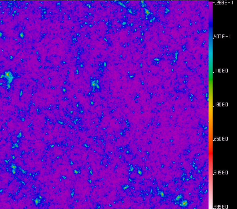
Figure 1: A noise-free $\kappa$ map in the N-body simulation of a WMAP cosmology with a width of 3 degrees and $2048^{2}$ pixels, and the scale is in units of $\kappa$.

We then simulate the CFHT Legacy Survey by adding noise to these clean maps. The noise $\kappa$ maps have a pixel-pixel variance $\sigma_{N}^{2}=\langle e^{2}\rangle/2/\langle N_{\rm pixel}\rangle=0.74^{2}$, which is the noise variance in each pixel before wiener filter. Here $\langle e^{2}\rangle=0.47^{2}$ is the total noise estimated in the VIRMOS-DESCART survey and here we take it as what would be expected by the CFHT Legacy Survey. It includes the dispersion of the galaxy intrinsic ellipticity, PSF correction noise and photon shot noise. $\langle N_{\rm pixel}\rangle$ is the mean number of galaxies in each pixel. For VIRMOS, the number density of observed galaxies $n_{g}\simeq 26/{\rm arcmin}^{2}$, then $\langle N_{\rm pixel}\rangle=n_{g}[(\theta_{\kappa}/1^{{}^{\prime}})/N]^{2}$, where $N=2048$ is the number of grids by which we store 2D maps and the field of view $\theta_{\kappa}$ is in units of arc min. The factor of 2 arises from the fact that the shear field has two degrees of freedom ($\gamma_{1},\gamma_{2}$), where the definition of $\langle e^{2}\rangle$ sums over both. We use this as our best guess for the CFHT Legacy Survey noise. We smooth both of the noise-free and noisy convergence fields by a Wiener filter $F_{W}$, so $\kappa_{W}(x)=\int\kappa(x^{\prime})F_{W}(x-x^{\prime})$. The Fourier transform of the Wiener filter is given by

$$F_{W}(k)=\frac{P^{S}(k)}{P^{S}(k)+P^{N}(k)}$$ (4)

where $P^{S}(k)$ is the power spectrum of the $\kappa$ field and $P^{N}(k)$ is the power spectrum of the noise. The broad Wiener filter smoothes the image, and reduces the variance of the noise per pixel. This can be revealed by the dotted line in Fig.(4), where the variance of pure Gaussian noise field smoothed with the Wiener filter is $\sigma_{Nf}=0.0084$. The Wiener filter has an effective area of $(\sigma_{N}/\sigma_{Nf})^{2}$ pixels. Of course, the pixels are highly correlated now.

The real $\kappa$ field is quite non-Gaussian, and a Wiener filter might not be the best. An alternative decomposition based on wavelets is discussed by Pen (1999).

Fig.(2) and (3) show the the noise-free and noisy $\kappa$ maps by adding simulated Gaussian noise field smoothed by Wiener filter respectively. It is apparent that even the minimum noise Wiener maps are very noisy, and where noise dominates salient features in the maps. The $\kappa$ field is equivalent to the E-mode of the shear field ($\gamma$), and a Wiener filter allows a direct mapping of the shear to filtered $\kappa$ field (Padmanabhan et al., 2003). It is well known that shear and kappa have equivalent noise properties (Seljak, 1998). This can be proven as follows: white and independent noise in $\gamma_{1}$ and $\gamma_{2}$, when Fourier transformed, is still white. The decomposition into E and B modes, i.e. the component of the shear in Fourier space that is parallel and perpendicular to the wave vector, is just a rotation of two uncorrelated noise variables. This gives two new uncorrelated noise variables of equal variance. The E mode and B mode will both have white noise again, which is statistically identical to the noise in $\gamma_{1}$ and $\gamma_{2}$ (differing by only a rotation). The E-mode is identical to kappa, except for one constant mode. Therefore kappa and shear can have their noise treated identically. For real surveys, the naive Wiener filter costs as the number of galaxies to the third power, and could be computationally very expensive, but fast $O(N)$ algorithms have already been demonstrated (Pen, 2003).

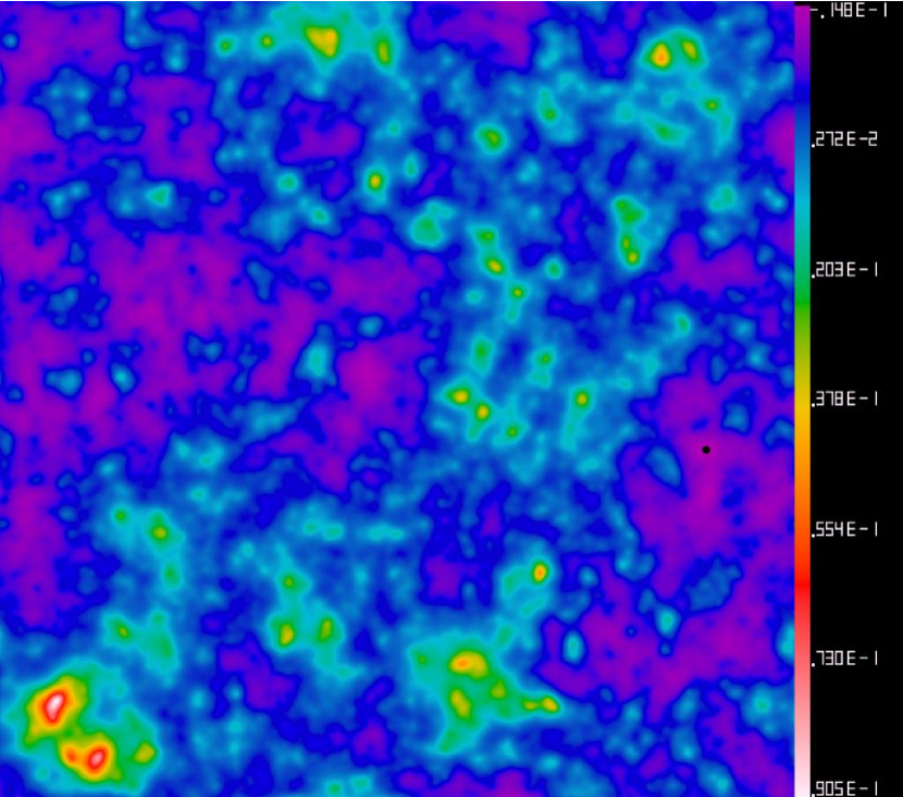
Figure 2: The same as Fig.1, but for the noise-free $\kappa$ map smoothed by a Wiener filter.

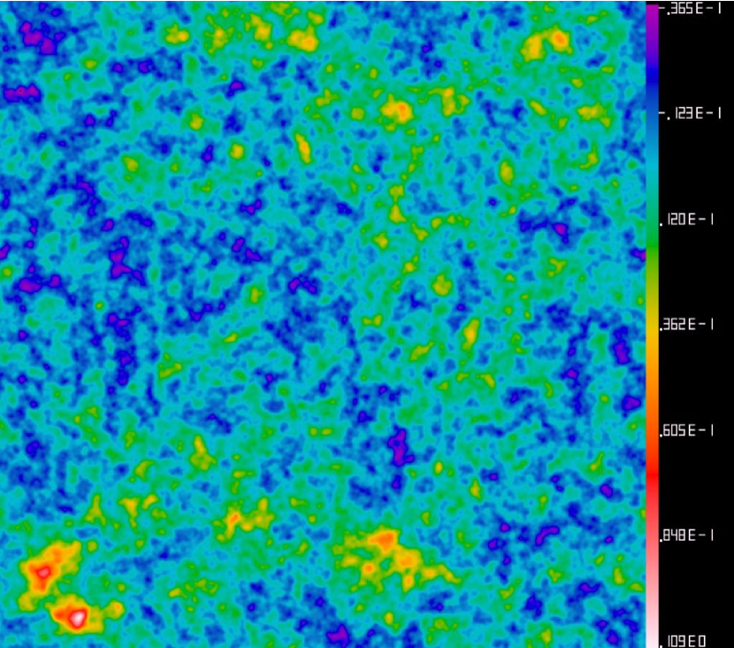
Figure 3: The same as Fig.2, but for noisy $\kappa$ map by adding a simulated Gaussian noise field smoothed with the same Wiener filter.

3 Wiener Reconstructing of the Convergence PDF

We apply Wiener filtering in two completely different contexts. In the previous sections, the Wiener filter was used to generate a minimum noise variance map. The next step is the tabulation of the PDF from a 9 square degree simulated survey field. This PDF is necessarily a noisy realization of the ensemble expectation value.

In addition to the sample variance noise, the observations themselves have noise. This is noise is added pointwise to the intrinsic lensing surface density. The PDF of the sum of signal plus noise is the convolution of the two PDF’s. We model the noise PDF as a Gaussian with zero mean and specified standard deviation. We further assume that the noise standard deviation is known.

In the ensemble average, one could in principle recover the lensing PDF from the noisy PDF by a deconvolution. In practice, of course, this is very difficult because the small scale noise is amplified by the deconvolution to the extent that it completely overwhelms the signal. Lee (2002) showed a heuristic scheme for noisy Sunyaev-Zeldovich measurements, which regularizes this deconvolution by applying a Wiener filter on the PDF of peaks. Lee extracted the “power spectrum” of the signal and noise in the PDF using Fourier transforms. Fourier transforms are good descriptions for stationary processes, but clearly a PDF is not a stationary process as a function of $\kappa$.

Stationarity is not a requirement for Wiener filtering. One can specify the full covariance matrix. However, one must be careful to formulate the question. What is meant by covariance? What is one approximating by a Gaussian process?

We first consider the literal interpretation. We define the ensemble average PDF of the 40 maps as the underlying PDF. The actual PDF of each map is a noisy realization. The difference of each map PDF from the ensemble average is the noise free signal variance.

Next, we consider a single map PDF with noise added. If the process of adding noise were an exact convolution, this would be a reversible process for a non-zero kernel, in particular for a Gaussian. To assess the actual contribution of noise, we take the noise-free PDF $P^{S}$, and convolve by the ideal noise kernel. Then we take the noisy map, and measure its actual noisy PDF $P^{S+N}$. The difference of the noisy map’s PDF from the ideal convolved PDF is a measure of the noise’s contribution on the irreversibility of the convolution. We thus define the noise covariance matrix as the covariance of the difference between the ideal convolved PDF and the noisy PDF of each map. The Wiener filtered deconvolution can then be readily applied to the observed noisy PDF, as we will demonstrate below.

One might wonder how circular this procedure really is. Our ultimate goal is to find a minimum noise measurement of the ensemble PDF from a noisy measurement of a single field PDF. In order to implement this, we had assumed prior knowledge of an ensemble of fields, as well as knowledge of the ensemble average $\kappa$ PDF and its covariance! At first sight this seems to imply much more prior knowledge than we set out to solve for. In practice, the problem is not as serious as it might sound. It needs to be shown that the actual assumed PDF for the signal is not important, or that it can be derived from the observed data alone.

We thus test not only the literal interpretation of a Wiener reconstructed PDF, but also of a more liberal version, we have assumed the signal PDF to be Gaussian. For a Gaussian, only the variance needs to be known or measured from the data, which can already be done to good accuracy from existing lensing data. The quality of the reconstruction will necessarily be worse, but we will show from actual simulations that good results can nevertheless be achieved.

The PDFs of pure $\kappa$ field, pure noise and $\kappa$ field added by noise are $P^{S}(\kappa)$, $P^{N}(\kappa)$ and $P^{S+N}(\kappa)$ respectively. The number of maps is $N=40$, i.e. $n=1,2,\cdots N$. Normally, PDFs are normalized to be unit, i.e. $\int^{+\infty}_{-\infty}P(\kappa)d\kappa=1$. From here on we only consider binned PDFs, choosing $M$ equally spaced bins separated by $\Delta\kappa$. Our notation becomes $\kappa_{i}=\kappa_{-}+i\Delta\kappa$, $P_{i}\equiv P(\kappa_{i})\Delta\kappa$, and each PDF can also carry an appropriate superscript. The number of bins for all PDFs is $M=19$, i.e. $i,j=1,2,\cdots M$.

In the form of matrix, $\mathbf{C}^{S}$ is the signal covariance and $\mathbf{C}^{N}$ is a noise covariance. The signal covariance is expressed as

$$C^{S}_{ij}=<[P^{S}_{i}-\bar{P}^{S}_{i}][P^{S}_{j}-\bar{P}^{S}_{j}]>,$$ (5)

where $<>$ is the average over 40 maps, and $\bar{P}^{S}(\kappa)$ is the average value of the $\kappa$ field PDF for 40 maps. The noise PDF, which will also serve as the noise convolution kernel $g^{N}(\kappa-\kappa^{\prime})$, is a Gaussian distribution

$$g^{N}(\kappa_{i}-\kappa_{j})=\frac{1}{\surd{2\pi}\sigma_{N}}\exp\left[-\frac{(\kappa_{i}-\kappa_{j})^{2}}{2\sigma^{2}_{N}}\right],$$ (6)

where $\sigma_{N}$ is the standard deviation of the noise after the wiener filter. We can also think of this kernel as a noise matrix $\mathbf{N}$

$$N_{ij}=g^{N}(\kappa_{i}-\kappa_{j})\Delta\kappa.$$ (7)

For a noisy $\kappa$ field, the noise deviation of the PDF relative to an invertible convolution can be written as for each map

$$\Delta P^{N}_{i}\equiv P^{S+N}_{i}-N_{ij}P^{S}_{j},$$ (8)

where $P^{S+N}(\kappa_{i})$ is the PDF of $\kappa$ field with added noise. Thus we have the noise covariance matrix

$$C^{N}_{ij}=<[\Delta P^{N}_{i}-\Delta\bar{P}^{N}_{i}][\Delta P^{N}_{j}-\Delta\bar{P}^{N}_{j}]>.$$ (9)

Using the convolution theorem, we have

$$P^{S+N}=\int^{+\infty}_{-\infty}P^{S}(\kappa^{\prime})g^{N}(\kappa-\kappa^{\prime})d\kappa,$$ (10)

$$P^{S+N}_{i}=\sum_{j=1}^{M}N_{ij}\cdot P^{S}_{j},$$ (11)

which reduces to in the form of matrix

$$\mathbf{\tilde{P}}^{S+N}=\mathbf{N}\mathbf{\tilde{P}}^{S},$$ (12)

so we have

$$\mathbf{\tilde{P}}^{S}=\mathbf{N}^{-1}\mathbf{\tilde{P}}^{S+N}.$$ (13)

The Wiener filter is defined as,

$$\mathbf{W}=\mathbf{C}^{S}(\mathbf{C}^{S}+\mathbf{\tilde{C}}^{N})^{-1},$$ (14)

where $\mathbf{\tilde{C}}^{N}=\mathbf{N}^{-1}\mathbf{C}^{N}\mathbf{N}^{-1}$.

All covariances are specified as deviations from a known underlying model. Given a the PDF of a noisy map, we then must first subtract the ensemble average noisy PDF, and apply the Wiener reconstruction to difference. After a applying a Wiener filtered deconvolution, we add back the noise free ensemble average PDF. The figure of merit is how well the reconstruction finds the noise-free PDF of the original map (not the ensemble average).

The reconstruction is thus decomposed into two parts: an underlying mean noisy PDF has a known pre-convolved (i.e. deconvolved) PDF. The difference between the map realization and this ensemble average is then deconvolved with a Wiener filter.

Expressed as equations, the deviation of reconstructed $\mathbf{\tilde{P}}^{S}_{W}$ is

$$\Delta\mathbf{\tilde{P}}^{S}_{W}=\mathbf{C}^{S}\mathbf{N}[\mathbf{N}\mathbf{C}^{S}\mathbf{N}+\mathbf{C}^{N}]^{-1}\Delta\mathbf{\tilde{P}}^{S+N}$$ (15)

where

$$\Delta\mathbf{\tilde{P}}^{S+N}=\mathbf{\tilde{P}}^{S+N}-\mathbf{\bar{\tilde{P}}}^{S+N};\ \ \mathbf{\bar{\tilde{P}}}^{S+N}=\mathbf{N}\mathbf{\bar{\tilde{P}}}^{S}.$$ (16)

Thus we can obtain the reconstructed $\mathbf{\tilde{P}}^{S}_{W}$

$$\mathbf{\tilde{P}}^{S}_{W}=\Delta\mathbf{\tilde{P}}^{S}_{W}+\mathbf{\bar{\tilde{P}}}^{S},$$ (17)

and its error

$$\mathbf{\sigma}^{2}_{\mathbf{\tilde{P}}^{S}_{W}}=<(\mathbf{\tilde{P}}^{S}_{W}-\mathbf{\tilde{P}}^{S})^{2}>,$$ (18)

where $<>$ is the mean over 40 maps, and $\mathbf{\tilde{P}}^{S}$ is the PDF of the $\kappa$ field.

A key assumption was that we actually knew the ensemble average PDF. The difference between the observed PDF and the ensemble average is a smaller amplitude function, and can be deconvolved using an appropriate Wiener filter. In practice, one might not know the underlying PDF, and subtract the wrong function. To test this possibility, we also used a Gaussian mean distribution for $\mathbf{\bar{\tilde{P}}}^{S}$ in equation (16). In the reconstructed PDF we again used the exact deconvolution of the Gaussian (which is of course also a Gaussian) $\mathbf{\bar{\tilde{P}}}^{S}$. In this case, we are applying the exact deconvolution to a lesser component of the observed PDF, and test how important it is to know the true underlying ensemble average PDF. One could in principle also use the signal covariance field of a Gaussian field in Equation (5). It does not appear as crucial a qualitative difference, and was not tested.

4 The reconstructed probability density function (PDF) and the cumulative distribution function (CDF)

The PDF of a convergence map is defined as

$$P(\kappa)=\frac{n(\Delta\kappa)}{N^{2}\Delta\kappa},$$ (19)

where $N$ is the number of grids by which 2D maps are stored and $n(\kappa)$ is the number of the within unit interval $\Delta\kappa$ of $\kappa$. Thus its corresponding cumulative distribution function (CDF) can be expressed as

$$C(>\kappa)=\int_{\kappa}P(\kappa^{\prime})d\kappa^{\prime}.$$ (20)

where $P(\kappa)$ is normalize to be unit in our analysis. Our purpose is to extract the PDF of $\kappa$ from noisy $\kappa$ map and compare it with that of pure convergence field, thus we can test the method mentioned in last section and apply it to the analysis of real week lensing data. Using the matrix method, we reconstruct the PDF of convergence from the pure, noisy $\kappa$ map and pure Gaussian noise smoothed by a Wiener filter. Fig.(4) plot the PDFs of the noise-free $\kappa$ field (solid line), noisy $\kappa$ field (dashed line) and pure Gaussian noise field (dotted line) respectively. The corresponding error bars are obtained from averaging over the 40 respective maps. The empty square dots represent the reconstructed PDF of the $\kappa$ field using the simulated pure $\kappa$ field as the initial signal field. We see that the reconstructed PDF of $\kappa$ is in good agreement with that of simulated pure $\kappa$ field, while there exists slight deviation for smaller negative and larger positive $\kappa$. Fig.(5) shows their corresponding CDFs.

In the reconstruction process, we used the PDF of the simulated pure $\kappa$ field as a initial signal field. However, in the real observation of weak lensing, the PDF of the pure convergence is unobservable. Thus we employ an approximation that the PDF $\bar{P}^{S}(\kappa_{j})$ of simulated convergence is replaced by a Gaussian distribution with mean standard deviation $\mathbf{\bar{\sigma}}_{\kappa}$ over 40 simulated $\kappa$ fields, because we can infer the mean standard deviation of $\kappa$ from the observational data of weak lensing. Fig.(6) and (7) plot the reconstructed PDFs and their corresponding CDFs using a Gaussian field with a mean standard deviation of 40 simulated pure $\kappa$ maps as an initial signal field, while Figs.(8) shows the relative errors of the PDF for the reconstructed $\kappa$ field using an initial signal field of a simulated pure $\kappa$ field (solid line) and a Gaussian field (dashed line) respectively. Apart from in smallest negative and largest positive convergence bins, the relative errors for the two initial PDF distributions are similar and about below 10$\%$. Therefore, using a Gaussian field PDF with a mean standard deviation of 40 simulated pure $\kappa$ maps as an initial signal field is a good approximation in the reconstruction of convergence PDF using this Wiener reconstruction approach.

Figure 4: The probability distribution functions (PDF) of the noise-free $\kappa$ field (solid line), noisy $\kappa$ field (dashed line) and pure Gaussian noise field (dotted line) respectively. The corresponding error bars are obtained from averaging over 40 respective maps. The empty square dots represent the reconstructed PDF of $\kappa$ field using simulated pure $\kappa$ field as a initial signal field.

Figure 5: The same as Fig.4, but for the corresponding cumulative distribution functions (CDF).

Figure 6: The same as Fig.4, but using a Gaussian field with a mean standard deviation of 40 simulated pure $\kappa$ maps as an initial signal field.

Figure 7: The same as Fig.6, but for the corresponding cumulative distribution functions (CDF).

Figure 8: The relative errors of PDF for reconstructed $\kappa$ field using an initial signal field of a simulated pure $\kappa$ field (solid line) and a Gaussian field (dashed line) respectively.

5 Conclusions and Discussions

In this letter, we ran a high-resolution N-body simulation of a WMAP cosmology to study the reconstruction of the convergence PDF from noisy weak lensing data. We added noise due to intrinsic ellipticity of background faint source galaxies to the simulated $\kappa$ fields and smoothed it using a Wiener filter. From the noisy simulated $\kappa$ field, we make the reconstruction of pdf of convergence by means of the PDF Wiener method described above. We find the reconstructed PDF of the convergence are in good agreement with that of a noise free $\kappa$ map smoothed by a Wiener filter, and its relative error is below about 10$\%$. We can safely apply this reconstructed method to the analysis of real observational data for week lensing such as future CFHT Legacy Survey.

We thank the anonymous referees for their many valuable suggestions. We also thank Ting-Ting Lu for providing the simulated lensing data and Hugh Merz for providing his simulation code. T.J.Zhang would like to thank Peng-Jie Zhang for useful discussion and Yuan Qiang for his help on MATLAB, and thank CITA, Xiang-Ping Wu, Xue-Lei Chen, Bo Qin and Da-Ming Chen for their hospitality during his visits to the Canadian Institute for Theoretical Astrophysics(CITA), University of Toronto and the cosmology groups of the National Astronomical Observatories of P.R.China, respectively. This work was partly supported by the National Science Foundation of China (Grants No.10473002 and 10273003), the 985 Project and the Scientific Research Foundation for the Returned Overseas Chinese Scholars, State Education Ministry. The research was also supported in part by NSERC and computational resources of the CFI funded infrastructure.

References

- Bacon et al. (2000) Bacon, D. J., Refregier, A. R., & Ellis, R. S. 2000, MNRAS, 318, 625
- Bennett et al. (2003) Bennett, C. L., Halpern, M., Hinshaw, G., Jarosik, N., Kogut, A., Limon, M., Meyer, S. S., Page, L., Spergel, D. N., Tucker, G. S., Wollack, E., Wright, E. L., Barnes, C., Greason, M. R., Hill, R. S., Komatsu, E., Nolta, M. R., Odegard, N., Peiris, H. V., Verde, L., & Weiland, J. L. 2003, ApJS, 148, 1
- Blandford et al. (1991) Blandford, R. D., Saust, A. B., Brainerd, T. G., & Villumsen, J. V. 1991, MNRAS, 251, 600
- Brown et al. (2003) Brown, M. L., Taylor, A. N., Bacon, D. J., Gray, M. E., Dye, S., Meisenheimer, K., & Wolf, C. 2003, MNRAS, 341, 100
- Gunn (1967) Gunn, J. E. 1967, ApJ, 147, 61
- Hamana et al. (2003) Hamana, T., Miyazaki, S., Shimasaku, K., Furusawa, H., Doi, M., Hamabe, M., Imi, K., Kimura, M., Komiyama, Y., Nakata, F., Okada, N., Okamura, S., Ouchi, M., Sekiguchi, M., Yagi, M., & Yasuda, N. 2003, ApJ, 597, 98
- Hoekstra et al. (2002) Hoekstra, H., Yee, H. K. C., Gladders, M. D., Barrientos, L. F., Hall, P. B., & Infante, L. 2002, ApJ, 572, 55
- Jain et al. (2000) Jain, B., Seljak, U., & White, S. 2000, ApJ, 530, 547
- Jarvis et al. (2003) Jarvis, M., Bernstein, G. M., Fischer, P., Smith, D., Jain, B., Tyson, J. A., & Wittman, D. 2003, AJ, 125, 1014
- Kaiser (1992) Kaiser, N. 1992, ApJ, 388, 272
- Lee (2002) Lee, J. 2002, ApJ, 578, L27
- Merz et al. (2004) Merz, H., Pen, U., & Trac, H. 2004, ArXiv Astrophysics e-prints: astro-ph/0402443
- Miralda-Escude (1991) Miralda-Escude, J. 1991, ApJ, 380, 1
- Padmanabhan et al. (2003) Padmanabhan, N., Seljak, U., & Pen, U. L. 2003, New Astronomy, 8, 581
- Pen (1999) Pen, U. 1999, Phil. Trans. Roy. Soc. London, A, 357, 2561
- Pen (2003) —. 2003, MNRAS, 346, 619
- Pen et al. (1994) Pen, U., Spergel, D. N., & Turok, N. 1994, Phys. Rev. D, 49, 692
- Pen et al. (2003) Pen, U., Zhang, T., van Waerbeke, L., Mellier, Y., Zhang, P., & Dubinski, J. 2003, ApJ, 592, 664
- Refregier et al. (2002) Refregier, A., Rhodes, J., & Groth, E. J. 2002, ApJ, 572, L131
- Seljak (1998) Seljak, U. 1998, ApJ, 506, 64
- Seljak & Zaldarriaga (1996) Seljak, U. & Zaldarriaga, M. 1996, ApJ, 469, 437+
- Van Waerbeke et al. (2002) Van Waerbeke, L., Mellier, Y., Pelló, R., Pen, U.-L., McCracken, H. J., & Jain, B. 2002, A&A, 393, 369
- Zhang et al. (2003) Zhang, T., Pen, U., Zhang, P., & Dubinski, J. 2003, ApJ, 598, 818