Multi-wavelength carbon recombination line observations with the VLA toward an UCH ii region in W48: Physical properties and kinematics of neutral material

Abstract

Using the Very Large Array (VLA) the C76$\alpha$ and C53$\alpha$ recombination lines (RLs) have been detected toward the ultra-compact H ii region (UCH ii region) G35.20$-$1.74. We also obtained upper limits to the carbon RLs at 6 cm (C110$\alpha$ & C111$\alpha$) and 3.6 cm (C92$\alpha$) wavelengths with the VLA. In addition, continuum images of the W48A complex ( which includes G35.20$-$1.74 ) are made with angular resolutions in the range 14″ to 2″. Modeling the multi-wavelength line and continuum data has provided the physical properties of the UCH ii region and the photodissociation region (PDR) responsible for the carbon RL emission. The gas pressure in the PDR, estimated using the derived physical properties, is at least four times larger than that in the UCH ii region. The dominance of stimulated emission of carbon RLs near 2 cm, as implied by our models, is used to study the relative motion of the PDR with respect to the molecular cloud and ionized gas. Our results from the kinematical study are consistent with a pressure-confined UCH ii region with the ionizing star moving with respect to the molecular cloud. However, based on the existing data, other models to explain the extended lifetime and morphology of UCH ii regions cannot be ruled out.

1 Introduction

Massive stars (OB stars) are formed by the gravitational collapse of clumps in molecular clouds. Lyman continuum ($E>13.6$ eV) photons from newly born OB stars ionize the surrounding material resulting in the formation of ultra-compact H ii regions (UCH ii regions). UCH ii regions are expected to expand due to their high gas pressure. If they expand at the speed of sound in the ionized gas, then the time taken for the UCH ii region to expand to $\sim$ 0.1 pc is a few times $10^{3}$ years. This time scale is referred to as the dynamical lifetime. However, the lifetime deduced from the observed number of UCH ii regions is a few times $10^{5}$ years. This discrepancy between the two lifetimes is referred to as the “lifetime problem” of UCH ii regions (Wood & Churchwell 1989a). Resolving the lifetime problem is an important step in understanding massive star formation in the Galaxy (see review by Garay & Lizano 1999).

There have been several suggestions to resolve the lifetime problem. In particular, De Pree, Rodríguez & Goss (1995) proposed that if high density ($\sim$ 10⁷ cm${}^{-3}~{}$), warm ($\sim$ 100 K) molecular material is present in the vicinity of UCH ii regions, it may be able to pressure confine UCH ii regions that form there and thus extend their lifetime. In the recent past, attempts have been made to observationally determine the physical properties of the molecular material near UCH ii regions. For example, Akeson & Carlstrom (1996) have used methyl cyanide, a good tracer of the temperature and density of dense molecular cores, to estimate the physical properties of the ambient medium near UCH ii regions G5.89+0.4 and G34.3+0.2. They concluded that the estimated ambient pressure ($>$ 10⁸ K cm${}^{-3}~{}$) was high enough to pressure confine the UCH ii regions. The dominant component of the ambient pressure need not always be the thermal pressure of the molecular gas but can be the turbulent pressure (Xie et al. 1996). Advances have also been made in modeling the dynamical evolution of UCH ii regions in the presence of high pressure molecular environment. Through simulations, Garcia-Segura & Franco (2004) show that pressure-confined UCH ii regions with ionizing stars moving with respect to the molecular core can be long-lived and can produce the observed morphologies of the H ii regions.

If UCH ii regions are pressure confined due to high density gas in their vicinity, then other observable effects will occur. In particular, far-ultraviolet (FUV) photons (6.0 – 13.6 eV) from the OB star would produce photo-dissociation regions (PDRs) in the neutral material close to the UCH ii region. Near the interface between the region where hydrogen is ionized and the PDR, gas phase carbon will be ionized by FUV photons in the energy range 11.3 to 13.6 eV (see review by Hollenbach & Tielens 1997). The electron density in this layer is relatively high ($>$ 10³ cm${}^{-3}~{}$) and gas temperatures can be in the range 300 – 1000 K (e.g. Natta, Walmsley & Tielens 1994). These conditions are ideally suited for producing observable radio recombination lines (RLs) of carbon.

Physical properties of dense material near UCH ii regions were earlier estimated from observations of high density molecular tracers. However, high line optical depth in these regions complicates the determination of the physical properties. We propose that multi-wavelength carbon RL observations from PDRs associated with UCH ii regions can be used to estimate the properties of the dense molecular material. Unlike molecular traces, RLs do not suffer from the limitation of high opacity and thus provide another probe to test whether UCH ii regions are pressure confined.

In this paper, we present multi-wavelength (0.7, 2, 3.6 & 6 cm) VLA observations of carbon RLs from the PDR associated with G35.20$-$1.74. The UCH ii region is in the molecular cloud complex W48 at $l=$ 35^o.2, $b=$ $-$1^o.74 at a distance of 3.2 kpc (Wood & Churchwell 1989b). At 0.7 cm, we have detected the C53$\alpha$ and X53$\alpha$ (see §4) transitions. This data forms the first successful imaging of carbon RL at 0.7 cm with the VLA at an angular resolution of about 2″. The details of the observations are given in §2. In §3 and §4, we discuss the modeling of the multi-wavelength data to determine the physical properties of the PDR and the UCH ii region. In §5, we estimate the gas pressure in the UCH ii region and the PDR and investigate whether the H ii region is pressure confined.

2 Observation and data reduction

We made spectroscopic observations of W48 using the VLA in D-configuration at 0.7, 2, 3.6 and 6 cm in dual polarization mode. The 0.7 cm observations were made during August 2004 and data at other wavelengths were obtained during October 2001. The transitions observed are the C110$\alpha$ (4876.5886 MHz) and C111$\alpha$ (4746.5497 MHz) at 6 cm, the C92$\alpha$ (8313.5279 MHz) at 3.6 cm, the C76$\alpha$ (14697.3141 MHz) at 2 cm, and the C53$\alpha$ (42973.3984 MHz) at 0.7 cm. The bandwidth at 2 cm wavelength was 3.13 MHz, which corresponds to a total velocity coverage of 64 km s^-1. Thus in addition to the carbon line, roughly 75 % of the He76$\alpha$ line profile falls within the observed bandwidth. Table 1 summarizes the parameters of the observations.

Data analysis was carried out using the Astronomical Image Processing Software (AIPS). The default channel zero data was used for continuum calibration. After satisfactory editing and calibration, the flag and calibration tables were transferred to the spectral data. The system band shapes were obtained using the bandpass calibrator data with the AIPS task BPASS. The estimated band shapes were used for bandpass calibration. Line free channels from the bandpass calibrated data were used for estimating the continuum emission which was then subtracted from the spectral line data. We used the task UVLSF for this purpose. The continuum uv data created by UVLSF was used as the input to IMAGR to make the continuum images. The spectral cubes were also made with the AIPS task IMAGR. The data at 0.7 cm were analyzed by taking into account of the weighting provided by the on-line system for each visibility measurement. GIPSY (Groningen Image Processing System) and AIPS++ software packages were used to further process (e.g. Gaussian fit) the spectral line data.

3 Continuum Emission

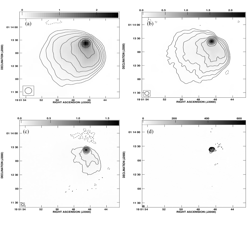
Figure 1: Continuum images of W48A (extended source) and the UCH ii region G35.20$-$1.74 (compact source) made with the VLA. (a) 6 cm image with an angular resolution of 14″.3 $\times$ 13″.0 ($-$0^o.8). The contour levels are ($-$1, 2, 5, 10, 20, 32, 64, 128, 256) $\times$ 10 mJy/beam and the grey scale ranges from $-$0.01 to 2.55 Jy/beam. The RMS noise in the image is 2.0 mJy/beam. (b) 3.6 cm image with an angular resolution of 8″.4 $\times$ 7″.6 ($-$17^o.2). The contour levels are ($-$1, 2, 5, 10, 20, 32, 64, 128, 256) $\times$ 5 mJy/beam and the grey scale ranges from $-$0.01 to 2.29 Jy/beam. The RMS noise in the image is 1.4 mJy/beam. (c) 2 cm image with an angular resolution of 4″.9 $\times$ 4″.5 (17^o.7). The contour levels are ($-$1, 2, 5, 10, 20, 32, 64, 128, 256) $\times$ 10 mJy/beam and the grey scale ranges from $-$0.01 to 1.67 Jy/beam. The RMS noise in the image is 2.9 mJy/beam. (d) 0.7 cm image with an angular resolution of 2″.1 $\times$ 2″.0 ($-$89^o.9). The contour levels are ($-$1, 2, 5, 10, 20, 32, 64, 128, 256) $\times$ 3 mJy/beam and the grey scale ranges from $-$4 to 630 mJy/beam. The RMS noise in the image is 0.7 mJy/beam.

Fig. 1 shows continuum images at 0.7, 2, 3.6 and 6 cm with angular resolutions ranging from $\sim$ 2″ to 14″. These continuum images show a compact source of angular size $\sim$ 5″ $\times$ 5″ along with an extended source (angular size $\sim$ 1′.5 $\times$ 1′.5), located south and east of the compact component (see Fig. 1). This extended source is designated as W48A in the literature (Onello et al.  1994). It has been suggested that the extended emission is directly associated with the compact component (Kurtz & Franco 2002).

The continuum emission and the partially ionized gas associated with W48A have been extensively studied earlier with a lower angular resolution of $\sim$ 60″ (see Onello et al. 1994). In our images, the emission from W48A extends to about 2′ at the longest wavelength. The flux densities of the extended emission measured are 5, 10 and 12 Jy respectively at 2, 3.6 and 6 cm wavelengths. The measured flux density at 2 cm is about a factor of two less than that estimated using the flux densities at 3.6 and 6 cm wavelengths and considering a spectral index of $-$0.1 for the thermal emission. This lower flux density is due to the missing short spacings in interferometric observations. The extended emission is not detected at 0.7 cm because of the same reason. The largest angular size that our observations are sensitive to are 5′, 3′, 1.5′ and 0.7′ respectively at 6, 3.6, 2 and 0.7 cm. Therefore at 2 and 0.7 cm wavelengths the full extent and flux density of the emission from W48A are not determined.

The compact source in Fig. 1 is an UCH ii region referred to as G35.20$-$1.74 in the literature (e.g. Wood and Churchwell 1989b). The continuum emission from G35.20$-$1.74 shows some resemblance to a cometary morphology as inferred earlier by Wood & Churchwell (1989b). The flux densities of the compact source at the four observed wavelengths are given in Table. 2. The angular size of the source is estimated from the 2 and 0.7 cm images, which have the highest angular resolutions. The AIPS task JMFIT was used to determine the angular size. The flux density and angular size are consistent with those estimated earlier (Wood & Churchwell 1989b, Woodward, Helfer & Pipher 1985).

The continuum data toward G35.20$-$1.74 are used to determine the physical properties of the UCH ii region. We model the continuum emission by considering that the emission from the compact source originates from a spherical, homogeneous ionized region. The flux density due to thermal emission from such an ionized region is estimated as described by Mezger & Henderson (1967). The angular size of the spherical region estimated from the observed size of the UCH ii region is 6″.3. Table 3 gives the parameters of the ionized gas obtained from continuum modeling. A plot of the flux density from the model as a function of frequency is shown in Fig. 2. At a distance of 3.2 kpc (Wood & Churchwell 1989b), the diameter of the spherical region of ionized gas is 0.1 pc. The derived physical properties and the observed flux densities are then used to estimate the excitation parameter, rate of Lyman continuum photons required to maintain ionization equilibrium and the spectral type of the embedded star (Panagia 1973). These values are also included in Table 3.

4 Recombination Line Emission toward G35.20$-$1.74

4.1 Carbon Recombination Lines

We detected the C53$\alpha$ and C76$\alpha$ recombination lines in the direction of G35.20$-$1.74. No carbon RLs were detected toward the extended H ii region W48A. The non-detections toward other directions indicate that the carbon line originates from the PDR associated with the UCH ii region. The spectra at 2 and 0.7 cm wavelengths, averaged over a 6″.3 $\times$ 6″.3 region near the continuum peak toward G35.20$-$1.74, are shown in Fig. 3 and the parameters obtained from the Gaussian fit to the line features in the figure are given in Table. 4. The upper limits on the carbon line emission at 3.6 and 6 cm are included in Table. 4. The data at 3.6 cm are affected by a systematic baseline ripple that was not removed by a careful bandpass calibration. This ripple is present in the spectra toward regions with bright continuum emission. The upper limit we obtained toward the UCHII region is from the spectrum with the baseline ripple and therefore its value is higher (5.2 mJy/beam) compared to that estimated from an off source position (= 1.1 mJy/beam).

4.2 Models for the Carbon line emission toward G35.20$-$1.74

We consider homogeneous ‘slabs’ of PDR material placed in front and back of the UCH ii region and solved the radiative transfer equation for non-LTE cases to obtain the recombination line flux density. The non-LTE departure coefficients $b_{n}$ and $\beta_{n}$ are calculated using the program originally developed by Brocklehurst & Salem (1977) and later modified by Walmsley & Watson (1982) and Payne, Anantharamaiah & Erickson (1994). The two relevant input parameters for the program are: (1) abundance of gas phase carbon and (2) background radiation field. The abundance of carbon is taken as 0.75 of the standard abundance (3.9 $\times$ 10^-4; Morton 1974), which implies a depletion factor of 25 % (Natta et al. 1994). The departure coefficients depend on the background radiation field. We have selected a thermal background due to an UCH ii region with temperature and emission measure determined from the continuum observations (see §3). The departure coefficients are computed for a set of electron temperatures in the range 100 to 1000 K and densities between 1000 and 6000 cm${}^{-3}~{}$. The dielectronic like recombination process that modifies the level population (Walmsley & Watson 1982) is also included in the calculation. The coefficients are computed by considering a 10000 level atom with the boundary condition $b_{n}\rightarrow 1$ at higher quantum states (see Payne et al. 1994 for further details).

The line intensity is a function of PDR gas temperature, $T_{PDR}$, electron density, $n_{e}^{PDR}$, PDR thickness along the line of sight, $l$, and the background radiation field. For the homogeneous PDR, the line brightness temperature, $T_{LB}$, due to the slab in the near side of the UCH ii region is given by (Shaver 1975)

$$T_{LB}=T_{bg,\nu}+T_{in,\nu}\ ,$$ (1)

where

$$T_{bg,\nu} = T_{0bg,\nu}e^{-\tau_{C\nu}}(e^{-\tau_{L\nu}}-1)\ ,$$

$$T_{in,\nu} = T_{PDR}\left(\frac{b_{m}\tau_{L\nu}^{*}+\tau_{C\nu}}{\tau_{L\nu}+\tau_{C\nu}}(1-e^{-(\tau_{L\nu}+\tau_{C\nu})})-(1-e^{-\tau_{C\nu}})\right).$$ (2)

$T_{bg,\nu}$ is the contribution to the line temperature due to the background radiation field and $T_{in,\nu}$ is the intrinsic line emission from the slab. In Eq. 2, $T_{0bg,\nu}$ is the background radiation temperature, which, as discussed above, is the continuum emission from the UCH ii region. $\tau_{C\nu}$ is the continuum optical depth of the PDR. The non-LTE line optical depth of the spectral transition from energy state $m$ to $n$, $\tau_{L\nu}$, is $\tau_{L\nu}=b_{n}\beta_{n}\tau_{L\nu}^{*}$ where $\tau_{L\nu}^{*}$ is the LTE line optical depth, $b_{n}$ and $\beta_{n}$ are the departure coefficients of state $n$. For the PDR, $\tau_{L\nu}^{*}\;\propto\;n_{e}^{PDR}n_{C^{+}}l$, where $n_{C^{+}}$ is the carbon ion volume number density in the PDR. For the present calculations we assumed that $n_{e}^{PDR}=n_{C^{+}}=n_{e}$ so $\tau_{L\nu}^{*}\;\propto\;n_{e}^{2}l$. The line temperature from the PDR on the far side (see below) is obtained from Eq. 1 by setting $T_{bg,\nu}=0$. The line brightness temperature is finally converted to flux density using an angular size of about 3″.7 (see Table 2).

We considered three classes of models – (a) models with line emission due to a PDR slab in the front of the UCH ii region; (b) models with line emission having contribution from PDR slabs in the front and back of the UCH ii region and (c) model with line emission due to a PDR slab in the far side of the UCH ii region. The line emission for class (a) models are obtained using Eqs. 1 and 2. For class (b) models, the intrinsic contribution (ie $T_{in,\nu}$ in Eq. 1) from the PDR slab on the far side is added to Eq. 1. Note that in this case we essentially assume that the relative motion between the PDR slabs in the front and back of the UCH ii region is smaller than the width of the observed carbon line (see §5.2). For each class of models, a set of parameter values is determined such that the observed line flux densities at 0.7 and 2 cm (also consistent with the observed upper limits at 3.6 and 6 cm) are reproduced within $\pm$ 1$\sigma$ error. We found that class (c) models cannot reproduce the observed line flux densities and hence will not be discussed further. Table 5 gives a subset of model parameters that are consistent with our RL data at the four wavelengths. The neutral densities listed in Table 5 are obtained with a gas phase carbon abundance of 3 $\times$ 10^-4 used for modeling. Fig. 4 shows the model carbon line flux density as a function of frequency along with the observed values and limits for class (a) and (b) models with typical temperatures 200 and 500 K and electron density 2500 cm${}^{-3}~{}$.

The modeling shows that: (1) the electron density and PDR thickness are well constrained by our RL data with the density in the range 1500 – 6000 cm${}^{-3}~{}$and the PDR thickness a few times 10^-4 pc; (2) models with temperatures $<$ 150 K are ruled out by our RL data. We have explored models with PDR temperatures up to 1000 K (Natta et al. 1994). However, the temperature could not be well constrained due to the uncertainty in the upper limit obtained from the 3.6 cm spectrum (see §4.1). Note that models with temperature $\leq$ 250 K are consistent with the 3$\sigma$ upper limit obtained from the off source region of 3.3 mJy at 3.6 cm (see Fig. 4).

In a recent single dish survey of carbon lines near 8.5 GHz, Roshi et al.  (2005) detected RLs toward a large number of UCH ii regions. These lines along with upper limits at other frequencies were used to model the properties of the line forming region. The ranges of density and size obtained for the PDR toward G35.2$-$1.74 are comparable with those determined by Roshi et al.  (2005) toward other UCH ii regions.

An important inference from modeling is that the line emission at frequencies near $\sim$ 14 GHz is dominated by stimulated emission due to the background continuum emission arising from the UCH ii region. The intrinsic line flux density from the slab near 14 GHz is $<$ 20 % of the observed RL flux density. Thus for these frequencies Eq. 1 can be approximated as $T_{LB}\sim T_{bg,\nu}$. At frequencies ${\mathrel{\mathchoice{\lower 2.9pt\vbox{\halign{$\m@th\displaystyle\hfil#\hfil$\cr>\crcr\sim\crcr}}}{\lower 2.9pt\vbox{\halign{$\m@th\textstyle\hfil#\hfil$\cr>\crcr\sim\crcr}}}{\lower 2.9pt\vbox{\halign{$\m@th\scriptstyle\hfil#\hfil$\cr>\crcr\sim\crcr}}}{\lower 2.9pt\vbox{\halign{$\m@th\scriptscriptstyle\hfil#\hfil$\cr>\crcr\sim\crcr}}}}}$14 GHz, the intrinsic line emission from the slab (ie $T_{in,\nu}$ in Eq. 1) contributes significantly. For example, at 0.7 cm the intrinsic line flux density from the PDR slab is about 6 mJy for models with electron density 3000 cm${}^{-3}~{}$, which is almost equal to the line flux density due to the background term (ie $T_{bg,\nu}$) in Eq. 1.

4.3 Helium and Other Recombination Lines

In addition to the C76$\alpha$ transition, He76$\alpha$ RLs in the direction of G35.20$-$1.74 and W48A were detected. The helium line parameters are given in Table 4. The LSR velocity of the He76$\alpha$ line ($+$42.0$\pm$0.5 km s^-1) differs by $-$5.9 km s^-1 from the earlier measured value for the H76$\alpha$ line (Wood & Churchwell 1989b). The parameters obtained for the H76$\alpha$ RL are $V_{LSR}$ = $+$47.9$\pm$1.2 km s^-1, $\Delta V$ = 31.8$\pm$1.89 km s^-1 and $S_{L}$ = 340$\pm$26 mJy. The angular resolution of our 2 cm observation is similar to that of the earlier observations ($\sim$ 4″; Wood & Churchwell 1989b). Differences in the sizes of the regions where helium and hydrogen are ionized could be the cause of the LSR velocity difference between the two RLs. The limited velocity coverage of the 2 cm data (see §2) could also be the cause of the LSR velocity difference. Further confirmation is needed however.

The line emission from W48A is averaged over an area of 36″ (in RA) $\times$ 17″ (in Dec) centered at RA(2000) 19^h01^m46^s.4 and DEC(2000) 01^o13${}^{{}^{\prime}}$02${}^{{}^{\prime\prime}}$. This region does not include the UCH ii region and thus is an estimate of the helium line emission from W48A. The line parameters given in Table 4 are from the average spectrum. The line flux density from W48A is only about 6 % of that toward the UCH ii region. The LSR velocity of the helium line from W48A ($+$47.4$\pm$0.5 km s^-1) is similar to that of the H76$\alpha$ line detected from G35.20$-$1.74 by Wood & Churchwell (1989b).

At 0.7 cm wavelength, a line feature at LSR velocity about $+$43.4 km s^-1 is detected. The LSR velocity is obtained by assuming that the mass of the ion to be infinity. Valee (1987) have detected the S125$\alpha$ recombination line toward W48A. However, the LSR velocity of the sulfur line ($+$43.1 km s^-1; Valee 1987) is similar to that of carbon lines detected in our observations. Therefore the second line feature detected at 0.7 cm wavelength may not be a sulfur line. The possibility of this line being a Doppler shifted carbon RL cannot be ruled out. Further investigation is needed to identify this line feature.

5 Is G35.20$-$1.74 pressure confined ?

As discussed in §1 the lifetime of UCH ii regions can be extended to a few times 10⁵ years if they are pressure confined. In this section, the derived physical properties of gas inside and outside G35.20$-$1.74 are used to investigate whether the UCH ii region is in fact pressure confined.

5.1 Estimation of gas pressure

The total gas pressure inside the UCH ii region is the sum of thermal pressure and turbulent pressure. No measurement of the magnetic field in G35.20$-$1.74 or the PDR associated with the H ii region exists and hence we do not include its contribution in the calculation of total pressure. The total gas pressure is given by

$$P_{uchii}=2kn_{e}T_{e}+n_{e}\mu m_{H}v_{H-turb}^{2}\mbox{~{}~{}dyne cm${}^{-2}$},$$ (3)

where $k$ is the Boltzmann constant, $n_{e}$ is the electron density in cm${}^{-3}~{}$, $T_{e}$ is the electron temperature in K, $m_{H}$ is the hydrogen mass in gm and $v_{H-turb}$ is the turbulent velocity inside the UCH ii region in units of cm s^-1. The line profile due to turbulence is considered to be Gaussian with $\sigma=v_{H-turb}$, which is estimated from the observed FWHM of H76$\alpha$ transition (Wood & Churchwell 1989b) and the calculated line width due to thermal motion. The effective mass in amu of H + He gas with He fraction in number of atoms taken as 10 % of that of H is 1.4. From the flux densities of H76$\alpha$ and He76$\alpha$ RLs we infer that about 8 % of the helium is ionized. Thus the parameter $\mu$ in the turbulent pressure term in Eq. 3 is $\sim$ 1.3 since it is expressed in terms of $n_{e}$. The values for electron density and temperature, estimated from modeling the continuum emission from the UCH ii region, are used to estimate gas pressure. The total pressure inside the UCH ii region is 1.3 $\times$ $10^{-7}$ dyne cm${}^{-2}~{}$, with a contribution of $7.0\times 10^{-8}$ dyne cm${}^{-2}~{}$from thermal process and $5.7\times 10^{-8}$ dyne cm${}^{-2}~{}$from turbulence. The turbulent pressure is about 85 % of the thermal pressure.

The total gas pressure in the PDR is given by

$$P_{PDR}=kn_{H}T_{PDR}+n_{H}\mu m_{H}v_{C-turb}^{2}\mbox{~{}~{}dyne cm${}^{-2}~{}$},$$ (4)

where $n_{H}$ is the number density of hydrogen atoms in cm${}^{-3}~{}$, $T_{PDR}$ is the PDR gas temperature in K, $v_{C-turb}$ is the turbulent velocity in cm s^-1. The line profile due to turbulence is considered to be Gaussian with $\sigma=v_{C-turb}$, which is estimated from the observed FWHM of C76$\alpha$ transition. The effective mass $\mu$ in amu is taken as 1.4. To estimate PDR pressure we consider that in the region where carbon is ionized, the neutral material is predominantly in atomic hydrogen form and the gas temperature is equal to the electron temperature estimated from carbon line modeling (see Hollenbach & Teilens 1997). The estimated total gas pressure in the PDR is between 5.3 $\times$ 10^-7 and 4.3 $\times$ 10^-6 dyne cm${}^{-2}~{}$for the model parameters given in Table 5. For PDR temperatures $\leq$ 500 K, the turbulent pressure is at least 10% more than the thermal pressure. This importance of turbulent pressure was noted earlier by Xie et al. (1996).

Comparing gas pressures in the UCH ii region and the PDR indicates that the pressure in the PDR is at least four times larger than that in the UCH ii region. In §5.2, we investigate the relative motion between the different components (ionized gas, material in the PDR and molecular gas) along the line-of-sight to understand this pressure difference.

5.2 Kinematics

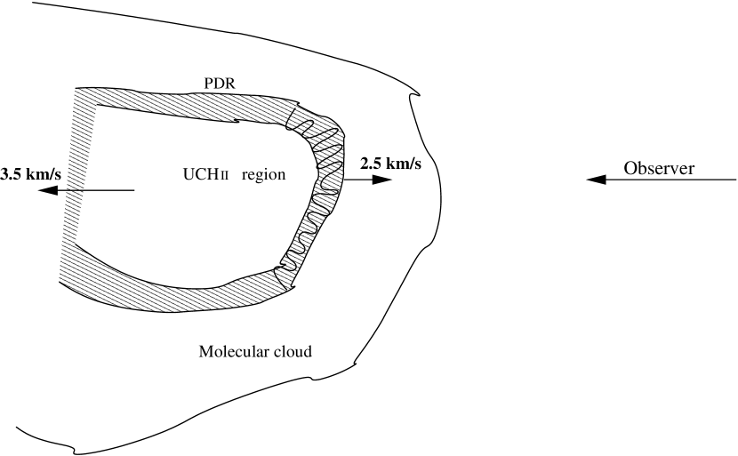
Figure 5: Schematic of the UCH ii region G35.20$-$1.74, the associated PDR and the molecular cloud. The hydrogen RL at 14.6 GHz originates from the UCH ii region. The central velocity of the H76$\alpha$ transition ($+$47.9$\pm$1.2 km s^-1) indicates the mean velocity of the ionized gas with respect to the LSR. The carbon RL observed at 14.6 GHz is detected from the region of the PDR marked by the curving line, since the line emission is dominated by stimulated emission. The central velocity of C76$\alpha$ line ($+$41.9$\pm$0.4 km s^-1). The mean LSR velocity of the observed molecular lines is $+$44.4$\pm$1.0 km s^-1. Thus relative to the molecular cloud the PDR is moving into the cloud at $-$2.5$\pm$1.1 km s^-1 and the ionized gas is moving at $+$3.5$\pm$1.6 km s^-1.

The UCH ii region G35.20$-$1.74 is located in the molecular cloud complex W48. The carbon line emission originates from PDR formed at the interface between the molecular cloud and the H ii region. The PDR resides within the molecular cloud. The relative motion along the line-of-sight between the three components (ionized gas, material in the PDR and molecular gas) can be determined by examining the central velocities of tracers of the different components (see Fig. 5). The central velocities of high density tracers of molecular gas observed toward G35.20$-$1.74 and the angular resolution of these observations are given in Table 6. The measured velocities with respect to the Local Standard of Rest (LSR) ranges from $+$42.8 to $+$46.1 km s^-1. (The errors in the central velocities are not given in the literature except for NH₃ (2,2), which is 0.1 km s^-1.) A variety of causes such as turbulence, shocks, complex excitation and chemistry in the vicinity of the UCH ii region contribute to the spread in the central velocity. Moreover, the different angular resolutions of the molecular line observations may also contribute to the velocity difference. Molecular line observations with higher angular resolution may help to precisely determine the LSR velocity of the cloud associated with the UCH ii region. Here we take the mean value ($+$44.4$\pm$1.0 km s^-1) of the central velocities listed in Table 6 as the LSR velocity of the molecular cloud.

The H76$\alpha$ line (Wood & Churchwell 1989b), which originates from the ionized gas in the UCH ii region (see §4.3), has a LSR velocity of $+$47.9$\pm$1.2 km s^-1. Since the UCH ii region is optically thin at 2 cm, this velocity provides the mean velocity of the ionized gas with respect to the LSR. As discussed in §4.2, the carbon RL flux density at 2 cm is dominated by stimulated emission and hence we preferentially observe the emission from the PDR in front (ie toward the observer; see Fig. 5) of the UCH ii region. The carbon RL at 2 cm has a central velocity of $+$41.9$\pm$0.4 km s^-1.

Translating the measured radial velocities to a reference frame at rest with respect to the molecular cloud gives the picture of the PDR moving into the molecular cloud at $-$2.5$\pm$1.1 km s^-1 and the ionized gas moving at $+$3.5$\pm$1.6 km s^-1 relative to the molecular cloud (see Fig. 5).

5.3 Discussion

Modeling the multi-wavelength ($\lambda=$ 0.7, 2, 3.6 & 6 cm) carbon recombination line and continuum data toward the UCH ii region G35.20$-$1.74 has provided the physical properties of the ionized gas and the PDR associated with the H ii region. These physical properties were then used to determine the pressure in the UCH ii region and the PDR in order to investigate whether the UCH ii region is pressure confined. Our calculations have shown that the pressure in the PDR is at least four times larger than that in the UCH ii region. Does this large pressure in the PDR indicate that the UCH ii region is pressure confined ? As shown in §5.2, the PDR moves relative to the molecular cloud at $-$2.5$\pm$1.1 km s^-1. This relative motion is inconsistent with a ‘stationary’ pressure-confined nebula where the H ii region is confined within the molecular cloud and the massive star ionizing the nebula is stationary with respect to the molecular cloud.

Garcia-Segura & Franco (2004) have considered the effects due to the natal molecular cloud gravity and stellar motion in their recent gas dynamical simulations. These simulations were done to study the evolution of pressure-confined H ii regions. They show that a plethora of structures for the ionized gas can be produced due to the stellar motion. In such models relative motions between the PDR, ionized gas and molecular cloud are expected both due to stellar motion and re-adjustments necessary for the ionized gas to be in hydrostatic equilibrium in the presence of cloud gravity. The PDR may reside in the shock formed as a result of stellar motion, which also explains the high pressure calculated in the PDR compared to the ionized gas. If the extended H ii region W48A is directly associated with G35.20$-$1.74 (Kurtz & Franco 2002), then, in this picture, the star has already moved into a density ramp in the molecular cloud which has resulted in the formation of the blister type region (Garcia-Segura & Franco 2004). However, other models that are proposed to explain the extended lifetime of UCH ii regions cannot be ruled out using the present data. For example, in the model by Kim & Koo (2001), where they combine the champagne flow model with the hierarchical structure of molecular cloud, relative motion of ionized gas with respect to the molecular cloud is expected due to the flow. It is possible that the PDR is moving with respect to the molecular cloud either because of stellar motion or due to increased pressure inside the H ii region caused by a stellar wind.

Table 1: Observational Parameters

	6 cm	3.6 cm	2 cm	0.7 cm
Date of observations	21-OCT-2001	21-OCT-2001	13-OCT-2001	13/17-AUG-2004
Field center RA (J2000)	19h01m47s.1	19h01m47s.1	19h01m46s.4	19h01m46s.4
Field center DEC (J2000)	+01o13${}^{{}^{\prime}}$00${}^{{}^{\prime\prime}}$	+01o13${}^{{}^{\prime}}$00${}^{{}^{\prime\prime}}$	+01o13${}^{{}^{\prime}}$24${}^{{}^{\prime\prime}}$	+01o13${}^{{}^{\prime}}$24${}^{{}^{\prime\prime}}$
RLs observed – IF1	C110$\alpha$	C92$\alpha$	C76$\alpha$, He76$\alpha$	C53$\alpha$
– IF2	C111$\alpha$
Center freq (GHz) – IF1	4.8754	8.3121	14.6927	42.9638
– IF2	4.7458
Bandwidth (MHz) – IF1	0.78	1.56	3.13	3.13
– IF2	0.78
Velocity range (km s-1) – IF1	48	56	64	42
– IF2	49
Channel separation (km s-1)
– IF1	0.75	0.88	1.0	1.4
– IF2	0.77
Phase calibrator	J1851+005	J1851+005	J1851+005	J1851+005
Bandpass calibrator	J1229+020	J1229+020	J1924$-$292	J1733$-$130
			J1733$-$130
Flux calibrator	3C 286	3C 286	3C 286	3C 286
On-source observing time (hrs)	1.6	1.8	4.0	2 $\times$ 3.3
Synthesized beam (arcsec)	14.3 $\times$ 13.0	8.4 $\times$ 7.6	4.9 $\times$ 4.5	2.1 $\times$ 2.0
Position angle of
synthesized beam (deg)	$-$0o.8	$-$17o.2	17o.7	$-$89o.9
Largest angular size (arcmin)	5	3	1.5	0.7
RMS noise in the spectral
cube (mJy/beam)	1.9	1.1	1.9	1.4
RMS noise in the
continuum images (mJy/beam)	2.0	1.4	2.9	0.7

Table 2: Parameters of G35.20$-$1.74 obtained from the continuum images

Obs. $\lambda$	Angular Size	Flux density
(cm)	(″)	(Jy)
0.7	3.7	2.21 (0.02)
2	3.6	2.49 (0.02)
4	$<$ 7.4	2.41 (0.02)
6	$<$ 15.7	1.95 (0.03)

Table 3: Physical properties of G35.20$-$1.74

Distance	size	Te	EM ($\times$ 107)	ne ($\times$ 104)	$U$	Log($N_{c}$)	Spectral Type
(kpc)	(pc)	(K)	(pc cm-6)	(cm-3)	(pc cm-2)	(s-1)
3.2	0.1	9900 (1400)	6.4 (0.3)	2.6	42.4	48.4	O8 – O7.5

Table 4: Parameters of the observed recombination lines

Obs. $\lambda$	Line	$S_{L}$	$\Delta V$	$V_{LSR}$	$V_{res}\tablenotemark{f}$	Effective Beam
(cm)		(mJy)	(km s-1)	(km s-1)	(km s-1)	(″$\times$ ″)
Toward G35.20$-$1.72
0.7	C53$\alpha$	14.7 (5.1)	5.5(2.2)	42.0(0.9)	1.4	6.3 $\times$ 6.3
	X53$\alpha$	80.0 (6.8)	3.1(0.3)	43.4(0.1)	—	—
2	C76$\alpha$	10.7 (1.6)	4.5(0.8)	41.9(0.4)	1.0	6.3 $\times$ 6.3
	He76$\alpha$	26.9(0.8)	21.2(1.3)	42.0(0.5)	—	—
3.6	C92$\alpha$	(5.2)			0.9	8.4 $\times$ 7.6 ($-$17o.26)
6	C110$\alpha$ &	(2.1)			0.8	14.4 $\times$ 13.0 ($-$0o.33)
	C111$\alpha$
Toward W48A
2	He76$\alpha$	1.4 (0.2)	14.8(1.1)	47.4(0.5)	1.0
3.6		(0.3)			0.9
6		(1.0)			0.8

Table 5: Physical properties of the PDR toward G35.20$-$1.74

TPDR	n${}_{e}^{PDR}$	$l$	$n_{H}$	PPDR
(K)	(cm-3)	($\times$ 10-4 pc)	($\times$ 106 cm-3)	($\times$ 10-7 dyne cm${}^{-2}~{}$)
Models with PDR slabs in front and back of the UCH ii region
150	1500 – 2000	0.8 – 0.5	5.1 – 6.8	5.3 – 7.1
200	1500 – 2500	1.2 – 0.6	5.1 – 8.6	5.6 – 9.4
300	1500 – 3000	2.6 – 0.8	5.1 – 10.3	6.2 – 12.5
500	1500 – 4000	5.3 – 1.0	5.1 – 13.7	7.5 – 20.0
1000	1500 – 4000	17.0 – 2.9	5.1 – 13.7	10.6 – 28.4
Models with a PDR slab in front of the UCH ii region
200	2000 – 2500	1.3 – 1.0	6.8 – 8.6	7.5 – 9.4
300	2000 – 4000	2.2 – 1.0	6.8 – 13.7	8.3 – 16.6
500	2000 – 5500	4.5 – 1.0	6.8 – 18.8	10.0 – 27.5
1000	2000 – 6000	14.0 – 2.6	6.8 – 20.5	14.2 – 42.6

Table 6: LSR velocity of high-density tracers observed toward G35.20$-$1.74

Molecular	$V_{LSR}$	$\theta_{res}$	References
transition	(km s-1)	(″)
13CO(1 $\rightarrow$ 0)	45.0	25	Churchwell et al. (1992)
13CO(2 $\rightarrow$ 1)	46.1	12	Churchwell et al. (1992)
NH3(1,1)	44.5	40	Churchwell et al. (1990)
NH3(2,2)	44.3	40	Churchwell et al. (1990)
CS (2 $\rightarrow$ 1)	42.8	25	Churchwell et al. (1992)
CS (5 $\rightarrow$ 4)	43.7	12	Churchwell et al. (1992)

Figure 2: Flux density vs frequency of the UCH ii region G35.20$-$1.74. The solid curve shows the model flux density as a function of frequency for $T_{e}=9900K$ and $EM=6.4\times 10^{7}$ pc cm^-6. The measured flux density at the four frequencies along with $\pm 3\sigma$ error bars are also marked.

Figure 3: Spectra of the 53$\alpha$ and 76$\alpha$ recombination line transitions observed near 2 (bottom) and 0.7 (top) cm toward G35.20$-$1.74. The spectra are obtained by averaging over a 6″.3 $\times$ 6″.3 region near the continuum peak (RA = 19^h01^m46^s.4, DEC = +01^o13${}^{{}^{\prime}}$24${}^{{}^{\prime\prime}}$, J2000) in the 2 and 0.7 cm images. The line features near $+$42 km s^-1 are the carbon lines. The He76$\alpha$ with an LSR velocity of $+$42.0$\pm$0.5 km s^-1 is the second feature in the spectrum shown on the bottom panel. Only part of the helium line profile is detected due to limited bandwidth of the observation. The line feature near $+$30 km s^-1 in the top spectrum is presumably a heavy ion (ion massive that C⁺) recombination line. The LSR velocity is with respect to the carbon lines. The result of a two component Gaussian fit to the line features is shown by the solid line.

Figure 4: Carbon line flux density as a function of frequency for class (a) and (b) models (see §4.2) are shown on Figs. (a) and (b) respectively. The solid and dashed curve corresponds to gas temperatures of 500 and 200 K respectively. The electron density used to obtain all curves are 2500 cm${}^{-3}~{}$. The upper limits at 6 and 3.6 cm wavelengths and the line flux densities of C53$\alpha$ and C76$\alpha$ transitions with $\pm$ 1$\sigma$ error are also marked. At frequencies below $\sim$ 10 GHz, the 200 K model predicts the carbon RLs in absorption. The parameters of such models are constrained by using the 6 cm spectral uncertainty (3$\sigma$) as a lower limit for the model flux densities at this wavelength, which is also shown in the figure. At 3.6 cm the upper limit obtained from off source spectra (3.3 mJy) is shown with a circle. Note that the 200 K model flux densities are consistent with this upper limit.

References

- (1) Akeson, R. L., Carlstrom, J. E., 1996, ApJ, 470, 528
- (2) Brocklehurst, M., Salem, M. 1977, Computer Phys. Commun., 13, 39
- (3) Churchwell, E., Walmsley, C. M., Wood, D. O. S., 1992, A&A, 253, 541
- (4) Churchwell, E., Walmsley, C. M., Cesaroni, R., 1990, A&AS, 83, 119
- (5) De Pree, C. G., Rodríguez, L. F., Goss, W. M., 1995, Rev. Mex. Astron. Astrofis, 31, 39
- (6) Garay, G., Lizano, S., 1999, PASP, 111, 1049
- (7) Garcia-Segura, G., Franco, J., 1996, ApJ, 469, 171
- (8) Garcia-Segura, G., Franco, J., 2004, Rev. Mex. Astron. Astrofis, 22, 131
- (9) Habing, H. J., 1968. Bull. Astron. Inst. Netherlands, 19, 421
- (10) Heiles, C., Chu, Y. H., 1980, ApJ, 235L, 105
- (11) Hollenbach, D. J., Tielens, A. G. G. M., 1997, ARA&A, 35, 179
- (12) Kim, K.-T., Koo, B.-C., 2001, ApJ, 549, 979
- (13) Kurtz, S. , Franco, J. , 2002, Rev. Mex. Astron. Astrofis, 12, 16
- (14) Mezger, P. G., Henderson, A. P., 1967, ApJ, 147, 471
- (15) Morton, D. C, 1974, ApJL 193, L35
- (16) Natta, A.; Walmsley, C. M.; Tielens, A. G. G. M. 1994, ApJ, 428, 209
- (17) Onello, J. S., Phillips, J. A., Benaglia, P., Goss, W. M., Terzian, Y., 1994, ApJ, 426, 249
- (18) Panagia, N., 1973, AJ, 78, 929
- (19) Payne H. E., Anantharamaiah K. R., Erickson W. C., 1994, ApJ, 430, 690
- (20) Roshi, D. A., et al. 2005, ApJ, in press
- (21) Shaver, P. A., 1975, Parmana, 5, 1
- (22) Vallee, J. P., 1987, ApJ, 317, 693
- (23) Walmsley C. M., Watson W. D., 1982, ApJ, 260, 317
- (24) Wood, D. O. S., Churchwell, E., 1989a, ApJ, 340, 265
- (25) Wood, D. O. S., Churchwell, E., 1989b, ApJS, 69, 831
- (26) Woodward, C. E., Helfer, H. L., Pipher, J. L., 1985, A&A, 147, 84
- (27) Xie, T., Mundy, L. G., Vogel, S. N., Hofner, P., 1996, ApJ, 473, L131