TASI Lectures on AstroParticle Physics

Abstract

astro-ph/0503065

UMN–TH–2346/05

FTPI–MINN–05/05

March 2005

Selected topics in Astroparticle Physics including the CMB, dark matter, BBN, and the variations of fundamental couplings are discussed.

1 Introduction

The background for all of the topics to be discussed in these lectures is the Big bang model. The observed homogeneity and isotropy enable us to describe the overall geometry and evolution of the Universe in terms of two cosmological parameters accounting for the spatial curvature and the overall expansion (or contraction) of the Universe. These two quantities appear in the most general expression for a space-time metric which has a (3D) maximally symmetric subspace of a 4D space-time, known as the Robertson-Walker metric:

$$ds^{2}=dt^{2}-R^{2}(t)\left[\frac{dr^{2}}{1-kr^{2}}+r^{2}(d\theta^{2}+\sin^{2}\theta d\phi^{2})\right]$$ (1)

where $R(t)$ is the cosmological scale factor and $k$ is the curvature constant. By rescaling the radial coordinate, we can choose $k$ to take only the discrete values $+1$, $-1$, or 0 corresponding to closed, open, or spatially flat geometries.

The cosmological equations of motion are derived from Einstein’s equations

$${\mathcal{R}}_{\mu\nu}-{1\over 2}g_{\mu\nu}{\mathcal{R}}=8\pi G_{\rm N}T_{\mu\nu}+\Lambda g_{\mu\nu}$$ (2)

where $\Lambda$ is the cosmological constant. It is common to assume that the matter content of the Universe is a perfect fluid, for which

$$T_{\mu\nu}=-pg_{\mu\nu}+\left(p+\rho\right)u_{\mu}u_{\nu}$$ (3)

where $g_{\mu\nu}$ is the space-time metric described by (1), $p$ is the isotropic pressure, $\rho$ is the energy density and $u=(1,0,0,0)$ is the velocity vector for the isotropic fluid in co-moving coordinates. With the perfect fluid source, Einstein’s equations lead to the Friedmann-Lemaître equations

$$H^{2}={{\dot{R}}^{2}\over R^{2}}={8\pi G_{\rm N}\rho\over 3}-{k\over R^{2}}+{\Lambda\over 3}$$ (4)

and

$$\frac{\ddot{R}}{R}=\frac{\Lambda}{3}-\frac{4\pi G_{\rm N}}{3}\;\;(\rho+3p)$$ (5)

where $H(t)$ is the Hubble parameter. Energy conservation via $T^{\mu\nu}_{~{};\mu}=0$, leads to a third useful equation [which can also be derived from Eqs. (4) and (5)]

$$\dot{\rho}=-3H\left(\rho+p\right)$$ (6)

The Friedmann equation can be rewritten as

$$(\Omega-1)H^{2}={k\over R^{2}}$$ (7)

so that $k=0,+1,-1$ corresponds to $\Omega=1,\Omega>1$ and $\Omega<1$. However, the value of $\Omega$ appearing in Eq. (7) represents the sum $\Omega=\Omega_{m}+\Omega_{\Lambda}$ of contributions from the matter density ($\Omega_{m}$) and the cosmological constant $(\Omega_{\Lambda}=\Lambda/3H^{2})$.

2 The CMB

There has been a great deal of progress in the last several years concerning the determination of both $\Omega_{m}$ and $\Omega_{\Lambda}$. Cosmic Microwave Background (CMB) anisotropy experiments have been able to determine the curvature (i.e. the sum of $\Omega_{m}$ and $\Omega_{\Lambda}$) to within a few percent, while observations of type Ia supernovae at high redshift provide information on a (nearly) orthogonal combination of the two density parameters.

The CMB is of course deeply rooted in the development and verification of the big bang model and big bang nucleosynthesis (BBN)[1]. Indeed, it was the formulation of BBN that led to the prediction of the microwave background. The argument is rather simple. BBN requires temperatures greater than 100 keV, which according to the standard model time-temperature relation, $t_{\rm s}T^{2}_{\rm MeV}=2.4/\sqrt{N}$, where $N$ is the number of relativistic degrees of freedom at temperature $T$, and corresponds to timescales less than about 200 s. The typical cross section for the first link in the nucleosynthetic chain is

$$\sigma v(p+n\rightarrow D+\gamma)\simeq 5\times 10^{-20}{\rm cm}^{3}/{\rm s}$$ (8)

This implies that it was necessary to achieve a density

$$n\sim{1\over\sigma vt}\sim 10^{17}{\rm cm}^{-3}$$ (9)

for nucleosynthesis to begin. The density in baryons today is known approximately from the density of visible matter to be ${n_{B}}_{o}\sim 10^{-7}$ cm^-3 and since we know that that the density $n$ scales as $R^{-3}\sim T^{3}$, the temperature today must be

$$T_{o}=({n_{B}}_{o}/n)^{1/3}T_{\rm BBN}\sim 10{\rm K}$$ (10)

thus linking two of the most important tests of the big bang theory.

An enormous amount of cosmological information is encoded in the angular expansion of the CMB temperature

$$T(\theta,\phi)=\sum_{\ell m}a_{\ell m}Y_{\ell m}(\theta,\phi).$$ (11)

The monopole term characterizes the mean background temperature of $T_{\gamma}=2.725\pm 0.001$ K as determined by COBE[2], whereas the dipole term can be associated with the Doppler shift produced by our peculiar motion with respect to the CMB. In contrast, the higher order multipoles, are directly related to energy density perturbations in the early Universe. When compared with theoretical models, the higher order anisotropies can be used to constrain several key cosmological parameters. In the context of simple adiabatic cold dark matter (CDM) models, there are nine of these: the cold dark matter density, $\Omega_{\chi}h^{2}$; the baryon density, $\Omega_{B}h^{2}$; the curvature - characterized by $\Omega_{\rm total}$; the hubble parameter, $h$; the optical depth, $\tau$; the spectral indices of scalar and tensor perturbations, $n_{s}$ and $n_{t}$; the ratio of tensor to scalar perturbations, $r$; and the overall amplitude of fluctuations, $Q$.

Microwave background anisotropy measurements have made tremendous advances in the last few years. The power spectrum[3, 4, 5, 6, 7, 8, 9, 10] has been measured relatively accurately out to multipole moments corresponding to $\ell\sim 2000$. A compilation of recent data is shown in Fig. 1 [11], where the power in at each ${\ell}$ is given by $(2{\ell}+1)C_{\ell}/(4\pi)$, and $C_{\ell}=<|a_{\ell m}|^{2}>$.

Figure 1: The power in the microwave background anisotropy spectrum as measured by WMAP[9], CBI[6], and ACBAR[10]. Taken from [11].

As indicated above, the details of this spectrum enable one to make accurate predictions of a large number of fundamental cosmological parameters. The results of the WMAP data (with other information concerning the power spectrum) is shown in Table 1. For details see ref. [9].

	WMAP alone	WMAPext $+$ 2dFGRS	WMAPext $+$ 2dFGRS $+$ Lyman $\alpha$
	power-law	power-law	running
$\Omega_{{\rm m}}h^{2}$	$0.14\pm 0.02$	$0.134\pm 0.006$	$0.135^{+0.008}_{-0.009}$
$\Omega_{{\rm B}}h^{2}$	$0.024\pm 0.001$	$0.023\pm 0.001$	$0.0224\pm 0.0009$
$h$	$0.72\pm 0.05$	$0.73\pm 0.03$	$0.71^{+0.04}_{-0.03}$
$n_{s}$	$0.99\pm 0.04$	$0.97\pm 0.03$	$0.93\pm 0.03$
$\tau$	$0.166^{+0.076}_{-0.071}$	$0.148^{+0.073}_{-0.071}$	$0.17\pm 0.06$

Of particular interest to us here is the CMB determination of the total density, $\Omega_{\rm tot}$, as well as the matter density $\Omega_{m}$. There is strong evidence that the Universe is flat or very close to it. The best constraint on $\Omega_{\rm total}$ is $1.02\pm 0.02$. Furthermore, the matter density is significantly larger than the baryon density implying the existence of cold dark matter and the baryon density, as we will see below, is consistent with the BBN production of D/H and its abundance in quasar absorption systems. The apparent discrepancy between the CMB value of $\Omega_{\rm tot}$ and $\Omega_{m}$, though not conclusive on its own, is a sign that a contribution from the vacuum energy density or cosmological constant, is also required. The preferred region in the $\Omega_{m}-\Omega_{\Lambda}$ plane is shown in Fig. 2 under four different assumptions[9].

Figure 2: Two-dimensional confidence regions in the ($\Omega_{\rm M},\Omega_{\Lambda}$) plane[9].

The presence or absence of a cosmological constant is a long standing problem in cosmology. We know that the cosmological term is at most a factor of a few times larger than the current mass density. Thus from Eq. (4), we see that the dimensionless combination, $G_{N}\Lambda\mathrel{\raise 1.29167pt\hbox{$<$\kern-7.5pt\lower 4.30554pt\hbox{$\sim$}}}10^{-121}$. Nevertheless, even a small non-zero value for $\Lambda$ could greatly affect the future history of the Universe: allowing open Universes to recollapse (if $\Lambda<0$), or closed Universes to expand forever (if $\Lambda>0$ and sufficiently large).

When the SN 1a results[12] are included (see the last panel of Fig. 2) we are led to a seemingly conclusive picture. The Universe is nearly flat with $\Omega_{\rm tot}\simeq 1$. However the density in matter makes up only 23% of this total, with the remainder in a cosmological constant or some other form of dark energy.

3 Dark Matter

3.1 Observational Evidence

Direct observational evidence for dark matter is found from a variety of sources. On the scale of galactic halos, the observed flatness of the rotation curves of spiral galaxies is a clear indicator for dark matter. There is also evidence for dark matter in elliptical galaxies, as well as clusters of galaxies coming from the X-ray observations of these objects. Also, direct evidence has been obtained through the study of gravitational lenses.

For example, assuming that galaxies are in virial equilibrium, one expects that one can relate the mass at a given distance $r$, from the center of a galaxy to its rotational velocity by

$$M(r)\propto v^{2}r/G_{N}$$ (12)

The rotational velocity, $v$, is measured[13, 14] by observing 21 cm emission lines in HI regions (neutral hydrogen) beyond the point where most of the light in the galaxy ceases. A subset of a compilation[15] of nearly 1000 rotation curves of spiral galaxies is shown in Fig. 3. The subset shown is restricted to a narrow range in brightness, but is characteristic for a wide range of spiral galaxies. Shown is the rotational velocity as a function of $r$ in units of the optical radius. If the bulk of the mass is associated with light, then beyond the point where most of the light stops, $M$ would be constant and $v^{2}\propto 1/r$. This is not the case, as the rotation curves appear to be flat, i.e., $v\sim$ constant outside the core of the galaxy. This implies that $M\propto r$ beyond the point where the light stops. This is one of the strongest pieces of evidence for the existence of dark matter on galactic scales. Velocity measurements indicate dark matter in elliptical galaxies as well[16]. For a more complete discussion see [17].

Figure 3: Synthetic rotation curve[15] for galaxies with $\langle M\rangle=-21.2$. The dotted curve shows the disk contribution, whereas the dashed curve shows the halo contribution.

3.2 Theory

Theoretically, there is no lack of support for the dark matter hypothesis. The standard big bang model including inflation almost requires $\Omega_{\rm tot}=1~{}$[18]. This can be seen from the following simple solution to the curvature problem. The unfortunate fact that at present we do not even know whether $\Omega$ is larger or smaller than one, indicates that we do not know the sign of the curvature term further implying that it is subdominant in Eq. (4)

$${k\over R^{2}}<{8\pi G\over 3}\rho$$ (13)

In an adiabatically expanding Universe, $R\sim T^{-1}$ where $T$ is the temperature of the thermal photon background. Therefore the quantity

$$\hat{k}={k\over R^{2}T^{2}}<{8\pi G\over 3T_{o}^{2}}<2\times 10^{-58}$$ (14)

is dimensionless and constant in the standard model. This is known as the curvature problem and can be resolved by a period of inflation. Before inflation, let us write $R=R_{i}$, $T=T_{i}$ and $R\sim T^{-1}$. During inflation, $R\sim T^{-1}\sim e^{Ht}$, where $H$ is constant. After inflation, $R=R_{f}\gg R_{i}$ but $T=T_{f}=T_{R}\mathrel{\raise 1.29167pt\hbox{$<$\kern-7.5pt\lower 4.30554pt\hbox{$\sim$}}}T_{i}$ where $T_{R}$ is the temperature to which the Universe reheats. Thus $R\not\sim T$ and $\hat{k}\rightarrow 0$ is not constant. But from Eqs. (7) and (14) if $\hat{k}\rightarrow 0$ then $\Omega\rightarrow 1$, and since typical inflationary models contain much more expansion than is necessary, $\Omega$ becomes exponentially close to one.

The existence of non-baryonic dark matter can be immediately inferred from the determination of the cosmological parameters through the microwave background anisotropy as described above. If $\Omega_{m}h^{2}\simeq 0.13$ and $\Omega_{B}h^{2}\simeq 0.02$, then the difference must be dark matter which contributes to the total density $\Omega_{\rm DM}h^{2}\simeq 0.11$. In addition, because the amplitude of fluctuations is relatively small, dark matter is necessary to have sufficient time to grow primordial perturbations into galaxies (for a more complete discussion see [17]).

3.3 Candidates

3.3.1 Baryons

Accepting the dark matter hypothesis, the first choice for a candidate should be something we know to exist, baryons. Though baryonic dark matter can not be the whole story if $\Omega_{m}>0.1$, the identity of the dark matter in galactic halos, which appear to contribute at the level of $\Omega\sim 0.05$, remains an important question needing to be resolved. A baryon density of this magnitude is not excluded by nucleosynthesis. Indeed we know some of the baryons are dark since $\Omega\mathrel{\raise 1.29167pt\hbox{$<$\kern-7.5pt\lower 4.30554pt\hbox{$\sim$}}}0.01$ in the disk of the galaxy.

It is interesting to note that until recently, there seemed to be some difficulty in reconciling the baryon budget of the Universe. By counting the visible contribution to $\Omega$ in stellar populations and the X-ray producing hot gas, Persic and Salucci[19] found only $\Omega_{\rm vis}\simeq 0.003$. A subsequent accounting by Fukugita, Hogan and Peebles[20] found slightly more ($\Omega\sim 0.02$) by including the contribution from plasmas in groups and clusters. At high redshift on the other hand, all of the baryons can be accounted for. The observed opacity of the Ly $\alpha$ forest in QSO absorption spectra requires a large baryon density consistent with the determinations by the CMB and BBN[21].

In galactic halos, however, it is quite difficult to hide large amounts of baryonic matter. Sites for halo baryons that have been discussed include Hydrogen (frozen, cold or hot gas), low mass stars/Jupiters, remnants of massive stars such as white dwarfs, neutron stars or black holes. In almost every case, a serious theoretical or observational problem is encountered[22].

3.3.2 Neutrinos

Light neutrinos ($m\leq 30eV$) are a long-time standard when it comes to non-baryonic dark matter[23]. Light neutrinos are, however, ruled out as a dominant form of dark matter because they produce too much large scale structure[24]. Because the smallest non-linear structures have mass scale $M_{J}\approx 3\times 10^{18}M_{\odot}/m_{\nu}^{2}({\rm eV})$ and the typical galactic mass scale is $\simeq 10^{12}M_{\odot}$, galaxies must fragment out of the larger pancake-like objects. The problem with such a scenario is that galaxies form late[25, 26] ($z\leq 1$) whereas quasars and galaxies are seen out to redshifts $z\mathrel{\raise 1.29167pt\hbox{$>$\kern-7.5pt\lower 4.30554pt\hbox{$\sim$}}}6$.

The neutrino decoupling scale of ${\mathcal{O}}(1)$ MeV has an important consequence on the final relic density of massive neutrinos. Neutrinos more massive than 1 MeV will begin to annihilate prior to decoupling, and while in equilibrium, their number density will become exponentially suppressed. Lighter neutrinos decouple as radiation on the other hand, and hence do not experience the suppression due to annihilation. Therefore, the calculations of the number density of light ($m_{\nu}\mathrel{\raise 1.29167pt\hbox{$<$\kern-7.5pt\lower 4.30554pt\hbox{$\sim$}}}1$ MeV) and heavy ($m_{\nu}\mathrel{\raise 1.29167pt\hbox{$>$\kern-7.5pt\lower 4.30554pt\hbox{$\sim$}}}1$ MeV) neutrinos differ substantially.

The energy of density of light neutrinos with $m_{\nu}\mathrel{\raise 1.29167pt\hbox{$<$\kern-7.5pt\lower 4.30554pt\hbox{$\sim$}}}1$ MeV can be expressed at late times as $\rho_{\nu}=m_{\nu}Y_{\nu}n_{\gamma}$ where $Y_{\nu}=n_{\nu}/n_{\gamma}$ is the number density of $\nu$’s relative to the density of photons, which today is 411 photons per cm³. It is easy to show that in an adiabatically expanding universe $Y_{\nu}=3/11$. This suppression is a result of the $e^{+}e^{-}$ annihilation which occurs after neutrino decoupling and heats the photon bath relative to the neutrinos. Imposing the constraint $\Omega_{\nu}h^{2}\mathrel{\raise 1.29167pt\hbox{$<$\kern-7.5pt\lower 4.30554pt\hbox{$\sim$}}}0.13$, translates into a strong constraint (upper bound) on Majorana neutrino masses[27]:

$$m_{\rm tot}=\sum_{\nu}m_{\nu}\mathrel{\raise 1.29167pt\hbox{$<$\kern-7.5pt\lower 4.30554pt\hbox{$\sim$}}}12{\rm eV}.$$ (15)

where the sum runs over neutrino mass eigenstates. The limit for Dirac neutrinos depends on the interactions of the right-handed states. The limit (15) and the corresponding initial rise in $\Omega_{\nu}h^{2}$ as a function of $m_{\nu}$ is displayed in the Figure 4.

Figure 4: Summary plot[28] of the relic density of Dirac neutrinos (solid) including a possible neutrino asymmetry of $\eta_{\nu}=5\times 10^{-11}$ (dotted).

Combining the rapidly improving data on key cosmological parameters with the better statistics from large redshift surveys has made it possible to go a step forward along this path. It is now possible to set stringent limits on the light neutrino mass density $\Omega_{\nu}h^{2}$, and hence on the neutrino mass based on the power spectrum of the Ly $\alpha$ forest[29], $m_{\rm tot}<5.5$ eV, and the limit is even stronger if the total matter density, $\Omega_{m}$ is less than 0.5. Adding additional observation constraints from the CMB and galaxy clusters drops this limit[30] to 4.2 eV. This limit has recently been improved by the 2dF Galaxy redshift[31] survey by comparing the derived power spectrum of fluctuations with structure formation models. Focussing on the the presently favoured $\Lambda$CDM model, the neutrino mass bound becomes $m_{\rm tot}<1.8$ eV for $\Omega_{m}<0.5$. When even more constraints such as HST Key project data, supernovae type Ia data, and BBN are included[32] the limit can be pushed to $m_{\rm tot}<0.9$ eV. With WMAP data, an upper limit of $m_{\rm tot}<0.7$ eV has been derived[9].

The calculation of the relic density for neutrinos more massive than $\sim 1$ MeV, is substantially more involved. The relic density is now determined by the freeze-out of neutrino annihilations which occur at $T\mathrel{\raise 1.29167pt\hbox{$<$\kern-7.5pt\lower 4.30554pt\hbox{$\sim$}}}m_{\nu}$, after annihilations have begun to seriously reduce their number density[33]. For particles which annihilate through approximate weak scale interactions, annihilations freeze out when $T\sim m_{\chi}/20$.

Roughly, the solution to the Boltzmann equation, which tracks the neutrino abundance, goes as $Y_{\nu}\sim f\sim(m\langle\sigma v\rangle_{ann})^{-1}$ and hence $\Omega_{\nu}h^{2}\sim{\langle\sigma v\rangle_{ann}}^{-1}$, so that parametrically $\Omega_{\nu}h^{2}\sim 1/{m_{\nu}^{2}}$. As a result, the constraint on $\Omega$ now leads to a lower bound[33, 34, 35] on the neutrino mass, of about $m_{\nu}\mathrel{\raise 1.29167pt\hbox{$>$\kern-7.5pt\lower 4.30554pt\hbox{$\sim$}}}3-7$ GeV, depending on whether it is a Dirac or Majorana neutrino. This bound and the corresponding downward trend $\Omega_{\nu}h^{2}\sim 1/m^{2}_{\nu}$ can again be seen in Figure 4. The result of a more detailed calculation is shown in Figure 5 [35] for the case of a Dirac neutrino. The two curves show the slight sensitivity on the temperature scale associated with the quark-hadron transition. The result for a Majorana mass neutrino is qualitatively similar. Indeed, any particle with roughly weak scale cross-sections will tend to give an interesting value of $\Omega h^{2}\sim 1$.

Figure 5: The relic density of heavy Dirac neutrinos due to annihilations[35]. The curves are labeled by the assumed quark-hadron phase transition temperature in MeV.

The deep drop in $\Omega_{\nu}h^{2}$, visible in Figure 4 at around $m_{\nu}=M_{Z}/2$, is due to a very strong annihilation cross section at $Z$-boson pole. For yet higher neutrino masses the $Z$-annihilation channel cross section drops as $\sim 1/m_{\nu}^{2}$, leading to a brief period of an increasing trend in $\Omega_{\nu}h^{2}$. However, for $m_{\nu}\mathrel{\raise 1.29167pt\hbox{$>$\kern-7.5pt\lower 4.30554pt\hbox{$\sim$}}}m_{W}$ the cross section regains its parametric form $\langle\sigma v\rangle_{ann}\sim m_{\nu}^{2}$ due to the opening up of a new annihilation channel to $W$-boson pairs[36], and the density drops again as $\Omega_{\nu}h^{2}\sim 1/m^{2}_{\nu}$. The tree level $W$-channel cross section breaks the unitarity at around ${\mathcal{O}}({\rm few})$ TeV [37] however, and the full cross section must be bound by the unitarity limit[38]. This behaves again as $1/m_{\nu}^{2}$, whereby $\Omega_{\nu}h^{2}$ has to start increasing again, until it becomes too large again at 200-400 TeV [38, 37].

If neutrinos are Dirac particles, and have a nonzero asymmetry the relic density could be governed by the asymmetry rather than by the annihilation cross section. Indeed, it is easy to see that the neutrino mass density corresponding to the asymmetry $\eta_{\nu}\equiv(n_{\nu}-n_{\bar{\nu}})/n_{\gamma}$ is given by[39] $\rho=m_{\nu}\eta_{\nu}n_{\gamma}$, which implies

$$\Omega_{\nu}h^{2}\simeq 0.004\,\eta_{\nu 10}\,(m_{\nu}/{\rm GeV}).$$ (16)

where $\eta_{\nu 10}\equiv 10^{10}\eta_{\nu}$. The behaviour of the energy density of neutrinos with an asymmetry is shown by the dotted line in the Figure 4. In the figure, we have assumed an asymmetry of $\eta_{\nu}\sim 5\times 10^{-11}$ for neutrinos with standard weak interaction strength.

Based on the leptonic and invisible width of the $Z$ boson, experiments at LEP have determined that the number of neutrinos is $N_{\nu}=2.994\pm 0.012$ [40]. Conversely, any new physics must fit within these brackets, and thus LEP excludes additional neutrinos (with standard weak interactions) with masses $m_{\nu}\mathrel{\raise 1.29167pt\hbox{$<$\kern-7.5pt\lower 4.30554pt\hbox{$\sim$}}}45$ GeV. Combined with the limits displayed in Figures 4 and 5, we see that the mass density of ordinary heavy neutrinos is bound to be very small, $\Omega_{\nu}{h}^{2}<0.001$ for masses $m_{\nu}>45$ GeV up to $m_{\nu}\sim{\mathcal{O}}(100)$ TeV. Lab constraints for Dirac neutrinos are available[41], excluding neutrinos with masses between 10 GeV and 4.7 TeV. This is significant, since it precludes the possibility of neutrino dark matter based on an asymmetry between $\nu$ and ${\bar{\nu}}$  [39].

3.3.3 Axions

Due to space limitations, the discussion of this candidate will be very brief. Axions are pseudo-Goldstone bosons which arise in solving the strong CP problem[42, 43] via a global U(1) Peccei-Quinn symmetry. The invisible axion[43] is associated with the flat direction of the spontaneously broken PQ symmetry. Because the PQ symmetry is also explicitly broken (the CP violating $\theta F{\widetilde{F}}$ coupling is not PQ invariant) the axion picks up a small mass similar to pion picking up a mass when chiral symmetry is broken. We can expect that $m_{a}\sim m_{\pi}f_{\pi}/f_{a}$ where $f_{a}$, the axion decay constant, is the vacuum expectation value of the PQ current and can be taken to be quite large. If we write the axion field as $a=f_{a}\theta$, near the minimum, the potential produced by QCD instanton effects looks like $V\sim m_{a}^{2}\theta^{2}f_{a}^{2}$. The axion equations of motion lead to a relatively stable oscillating solution. The energy density stored in the oscillations exceeds the critical density[44] unless $f_{a}\mathrel{\raise 1.29167pt\hbox{$<$\kern-7.5pt\lower 4.30554pt\hbox{$\sim$}}}10^{12}$ GeV.

Axions may also be emitted stars and supernova[45]. In supernovae, axions are produced via nucleon-nucleon bremsstrahlung with a coupling $g_{A}N\propto m_{N}/f_{a}$. As was noted above the cosmological density limit requires $f_{a}\mathrel{\raise 1.29167pt\hbox{$<$\kern-7.5pt\lower 4.30554pt\hbox{$\sim$}}}10^{12}$ GeV. Axion emission from red giants imply[46] $f_{a}\mathrel{\raise 1.29167pt\hbox{$>$\kern-7.5pt\lower 4.30554pt\hbox{$\sim$}}}10^{10}$ GeV (though this limit depends on an adjustable axion-electron coupling), the supernova limit requires[47] $f_{a}\mathrel{\raise 1.29167pt\hbox{$>$\kern-7.5pt\lower 4.30554pt\hbox{$\sim$}}}2\times 10^{11}$ GeV for naive quark model couplings of the axion to nucleons. Thus only a narrow window exists for the axion as a viable dark matter candidate.

4 Supersymmetric Dark Matter

For the remaining discussion of dark matter, I will restrict my attention to supersymmetry and in particular, the minimal supersymmetric standard model (MSSM) with R-parity conservation. R-parity is necessary if one wants to forbid all new baryon and lepton number violating interactions at the weak scale. If R-parity, which distinguishes between “normal” matter and the supersymmetric partners and can be defined in terms of baryon, lepton and spin as $R=(-1)^{3B+L+2S}$, is unbroken, there is at least one supersymmetric particle (the lightest supersymmetric particle or LSP) which must be stable. Thus, the minimal model contains the fewest number of new particles and interactions necessary to make a consistent theory.

There are very strong constraints, however, forbidding the existence of stable or long lived particles which are not color and electrically neutral[48]. Strong and electromagnetically interacting LSPs would become bound with normal matter forming anomalously heavy isotopes. Indeed, there are very strong upper limits on the abundances, relative to hydrogen, of nuclear isotopes[49], $n/n_{H}\mathrel{\raise 1.29167pt\hbox{$<$\kern-7.5pt\lower 4.30554pt\hbox{$\sim$}}}10^{-15}~{}~{}{\rm to}~{}~{}10^{-29}$ for 1 GeV $\mathrel{\raise 1.29167pt\hbox{$<$\kern-7.5pt\lower 4.30554pt\hbox{$\sim$}}}m\mathrel{\raise 1.29167pt\hbox{$<$\kern-7.5pt\lower 4.30554pt\hbox{$\sim$}}}$ 1 TeV. A strongly interacting stable relic is expected to have an abundance $n/n_{H}\mathrel{\raise 1.29167pt\hbox{$<$\kern-7.5pt\lower 4.30554pt\hbox{$\sim$}}}10^{-10}$ with a higher abundance for charged particles.

There are relatively few supersymmetric candidates which are not colored and are electrically neutral. The sneutrino[50] is one possibility, but in the MSSM, it has been excluded as a dark matter candidate by direct[41] and indirect[51] searches. In fact, one can set an accelerator based limit on the sneutrino mass from neutrino counting, $m_{\tilde{\nu}}\mathrel{\raise 1.29167pt\hbox{$>$\kern-7.5pt\lower 4.30554pt\hbox{$\sim$}}}$ 44.7 GeV [52]. In this case, the direct relic searches in underground low-background experiments require $m_{\tilde{\nu}}\mathrel{\raise 1.29167pt\hbox{$>$\kern-7.5pt\lower 4.30554pt\hbox{$\sim$}}}$ 20 TeV [41]. Another possibility is the gravitino which is probably the most difficult to exclude. I will concentrate on the remaining possibility in the MSSM, namely the neutralinos but will return to the case of gravitino dark matter as well.

4.1 Parameters

The most general version of the MSSM, despite its minimality in particles and interactions contains well over a hundred new parameters. The study of such a model would be untenable were it not for some (well motivated) assumptions. These have to do with the parameters associated with supersymmetry breaking. It is often assumed that, at some unification scale, all of the gaugino masses receive a common mass, $m_{1/2}$. The gaugino masses at the weak scale are determined by running a set of renormalization group equations. Similarly, one often assumes that all scalars receive a common mass, $m_{0}$, at the GUT scale. These too are run down to the weak scale. The remaining supersymmetry breaking parameters are the trilinear mass terms, $A_{0}$, which I will also assume are unified at the GUT scale, and the bilinear mass term $B$. There are, in addition, two physical CP violating phases which will not be considered here. Finally, there is the Higgs mixing mass parameter, $\mu$, and since there are two Higgs doublets in the MSSM, there are two vacuum expectation values. One combination of these is related to the $Z$ mass, and therefore is not a free parameter, while the other combination, the ratio of the two vevs, $\tan\beta$, is free.

The natural boundary conditions at the GUT scale for the MSSM would include $\mu$ and $B$ in addition to $m_{1/2}$, $m_{0}$, and $A_{0}$. In this case, upon running the RGEs down to a low energy scale and minimizing the Higgs potential, one would predict the values of $M_{Z}$, $\tan\beta$ (in addition to all of the sparticle masses). Since $M_{Z}$ is known, it is more useful to analyze supersymmetric models where $M_{Z}$ is input rather than output. It is also common to treat $\tan\beta$ as an input parameter. This can be done at the expense of shifting $\mu$ (up to a sign) and $B$ from inputs to outputs. This model is often referred to as the constrained MSSM or CMSSM. Once these parameters are set, the entire spectrum of sparticle masses at the weak scale can be calculated.

Figure 6: RG evolution of the mass parameters in the CMSSM.

In Fig. 6, an example of the running of the mass parameters in the CMSSM is shown. Here, we have chosen $m_{1/2}=250$ GeV, $m_{0}=100$ GeV, $\tan\beta=3$, $A_{0}=0$, and $\mu<0$. Indeed, it is rather amazing that from so few input parameters, all of the masses of the supersymmetric particles can be determined. The characteristic features that one sees in the figure, are for example, that the colored sparticles are typically the heaviest in the spectrum. This is due to the large positive correction to the masses due to $\alpha_{3}$ in the RGE’s. Also, one finds that the ${\widetilde{B}}$ (the partner of the $U(1)_{Y}$ gauge boson), is typically the lightest sparticle. But most importantly, notice that one of the Higgs mass², goes negative triggering electroweak symmetry breaking[53]. (The negative sign in the figure refers to the sign of the mass², even though it is the mass of the sparticles which are depicted.)

4.2 Neutralinos

There are four neutralinos, each of which is a linear combination of the $R=-1$ neutral fermions[48]: the wino $\tilde{W}^{3}$, the partner of the 3rd component of the $SU(2)_{L}$ gauge boson; the bino, $\tilde{B}$; and the two neutral Higgsinos, $\tilde{H}_{1}$ and $\tilde{H}_{2}$. Assuming gaugino mass universality at the GUT scale, the identity and mass of the LSP are determined by the gaugino mass $m_{1/2}$, $\mu$, and $\tan\beta$. In general, neutralinos can be expressed as a linear combination

$$\chi=\alpha\tilde{B}+\beta\tilde{W}^{3}+\gamma\tilde{H}_{1}+\delta\tilde{H}_{2}$$ (17)

The solution for the coefficients $\alpha,\beta,\gamma$ and $\delta$ for neutralinos that make up the LSP can be found by diagonalizing the mass matrix

$$({\tilde{W}}^{3},{\tilde{B}},{{\tilde{H}}^{0}}_{1},{{\tilde{H}}^{0}}_{2})\left(\begin{array}[]{cccc}M_{2}&0&{-g_{2}v_{1}\over\sqrt{2}}&{g_{2}v_{2}\over\sqrt{2}}\\ 0&M_{1}&{g_{1}v_{1}\over\sqrt{2}}&{-g_{1}v_{2}\over\sqrt{2}}\\ {-g_{2}v_{1}\over\sqrt{2}}&{g_{1}v_{1}\over\sqrt{2}}&0&-\mu\\ {g_{2}v_{2}\over\sqrt{2}}&{-g_{1}v_{2}\over\sqrt{2}}&-\mu&0\end{array}\right)\left(\begin{array}[]{c}{\tilde{W}}^{3}\\ {\tilde{B}}\\ {{\tilde{H}}^{0}}_{1}\\ {{\tilde{H}}^{0}}_{2}\end{array}\right)$$ (18)

where $M_{1}(M_{2})$ is a soft supersymmetry breaking term giving mass to the U(1) (SU(2)) gaugino(s). In a unified theory $M_{1}=M_{2}=m_{1/2}$ at the unification scale (at the weak scale, $M_{1}\simeq{5\over 3}{\alpha_{1}\over\alpha_{2}}M_{2}$). As one can see, the coefficients $\alpha,\beta,\gamma,$ and $\delta$ depend only on $m_{1/2}$, $\mu$, and $\tan\beta$. In the CMSSM, the solutions for $\mu$ generally lead to a lightest neutralino which is very nearly a pure $\tilde{B}$.

4.3 The Relic Density

The relic abundance of LSP’s is determined by solving the Boltzmann equation for the LSP number density in an expanding Universe. The technique[35] used is similar to that for computing the relic abundance of massive neutrinos[33] with the appropriate substitution of the cross section. The relic density depends on additional parameters in the MSSM beyond $m_{1/2},\mu$, and $\tan\beta$. These include the sfermion masses, $m_{\tilde{f}}$ and the Higgs pseudo-scalar mass, $m_{A}$, derived from $m_{0}$ (and $m_{1/2}$). To determine the relic density it is necessary to obtain the general annihilation cross-section for neutralinos. In much of the parameter space of interest, the LSP is a bino and the annihilation proceeds mainly through sfermion exchange. Because of the p-wave suppression associated with Majorana fermions, the s-wave part of the annihilation cross-section is suppressed by the outgoing fermion masses. This means that it is necessary to expand the cross-section to include p-wave corrections which can be expressed as a term proportional to the temperature if neutralinos are in equilibrium. Unless the neutralino mass happens to lie near near a pole, such as $m_{\chi}\simeq$ $m_{Z}/2$ or $m_{h}/2$, in which case there are large contributions to the annihilation through direct $s$-channel resonance exchange, the dominant contribution to the $\tilde{B}\tilde{B}$ annihilation cross section comes from crossed $t$-channel sfermion exchange.

Annihilations in the early Universe continue until the annihilation rate $\Gamma\simeq\sigma vn_{\chi}$ drops below the expansion rate. The final neutralino relic density expressed as a fraction of the critical energy density can be written as[48]

$$\Omega_{\chi}h^{2}\simeq 1.9\times 10^{-11}\left({T_{\chi}\over T_{\gamma}}\right)^{3}N_{f}^{1/2}\left({{\rm GeV}\over ax_{f}+{1\over 2}bx_{f}^{2}}\right)$$ (19)

where $(T_{\chi}/T_{\gamma})^{3}$ accounts for the subsequent reheating of the photon temperature with respect to $\chi$, due to the annihilations of particles with mass $m<x_{f}m_{\chi}$ [54] and $x_{f}=T_{f}/m_{\chi}$ is proportional to the freeze-out temperature. The coefficients $a$ and $b$ are related to the partial wave expansion of the cross-section, $\sigma v=a+bx+\dots$. Eq. (19 ) results in a very good approximation to the relic density expect near s-channel annihilation poles, thresholds and in regions where the LSP is nearly degenerate with the next lightest supersymmetric particle[55].

4.4 The CMSSM after WMAP

For a given value of $\tan\beta$, $A_{0}$, and $sgn(\mu)$, the resulting regions of acceptable relic density and which satisfy the phenomenological constraints can be displayed on the $m_{1/2}-m_{0}$ plane. In Fig. 7a, the light shaded region corresponds to that portion of the CMSSM plane with $\tan\beta=10$, $A_{0}=0$, and $\mu>0$ such that the computed relic density yields $0.1<\Omega_{\chi}h^{2}<0.3$. At relatively low values of $m_{1/2}$ and $m_{0}$, there is a large ‘bulk’ region which tapers off as $m_{1\!/2}$ is increased. At higher values of $m_{0}$, annihilation cross sections are too small to maintain an acceptable relic density and $\Omega_{\chi}h^{2}>0.3$. Although sfermion masses are also enhanced at large $m_{1\!/2}$ (due to RGE running), co-annihilation processes between the LSP and the next lightest sparticle (in this case the ${\widetilde{\tau}}_{\scriptscriptstyle\rm 1}$) enhance the annihilation cross section and reduce the relic density. This occurs when the LSP and NLSP are nearly degenerate in mass. The dark shaded region has $m_{{\widetilde{\tau}}_{\scriptscriptstyle\rm 1}}<m_{\chi}$ and is excluded. Neglecting coannihilations, one would find an upper bound of $\sim 450{\rm\,Ge\kern-1.25ptV}$ on $m_{1\!/2}$, corresponding to an upper bound of roughly $200{\rm\,Ge\kern-1.25ptV}$ on $m_{\tilde{B}}$. The effect of coannihilations is to create an allowed band about 25-50 ${\rm\,Ge\kern-1.25ptV}$ wide in $m_{0}$ for $m_{1\!/2}\mathrel{\raise 1.29167pt\hbox{$<$\kern-7.5pt\lower 4.30554pt\hbox{$\sim$}}}1400{\rm\,Ge\kern-1.25ptV}$, which tracks above the $m_{\tilde{\tau}_{1}}=m_{\chi}$ contour[56].

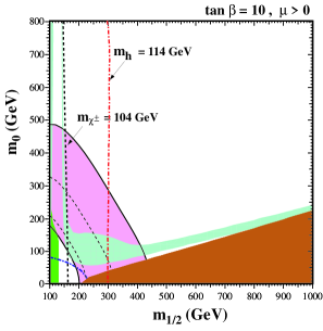
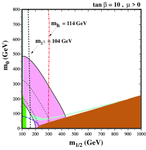
Figure 7: The $(m_{1/2},m_{0})$ planes for (a) $\tan\beta=10$ and $\mu>0$, assuming $A_{0}=0,m_{t}=175$ GeV and $m_{b}(m_{b})^{\overline{MS}}_{SM}=4.25$ GeV. The near-vertical (red) dot-dashed lines are the contours $m_{h}=114$ GeV, and the near-vertical (black) dashed line is the contour $m_{\chi^{\pm}}=104$ GeV. Also shown by the dot-dashed curve in the lower left is the corner excluded by the LEP bound of $m_{\tilde{e}}>99$ GeV. The medium (dark green) shaded region is excluded by $b\to s\gamma$, and the light (turquoise) shaded area is the cosmologically preferred regions with $0.1\leq\Omega_{\chi}h^{2}\leq 0.3$. In the dark (brick red) shaded region, the LSP is the charged ${\tilde{\tau}}_{1}$. The region allowed by the E821 measurement of $a_{\mu}$ at the 2-$\sigma$ level, is shaded (pink) and bounded by solid black lines, with dashed lines indicating the 1-$\sigma$ ranges. In (b), the relic density is restricted to the range $0.094<\Omega_{\chi}h^{2}<0.129$.

Also shown in Fig. 7a are the relevant phenomenological constraints. These include the limit on the chargino mass: $m_{\chi^{\pm}}>104$ GeV [57], on the selectron mass: $m_{\tilde{e}}>99$ GeV  [58] and on the Higgs mass: $m_{h}>114$ GeV [59]. The former two constrain $m_{1/2}$ and $m_{0}$ directly via the sparticle masses, and the latter indirectly via the sensitivity of radiative corrections to the Higgs mass to the sparticle masses, principally $m_{\tilde{t},\tilde{b}}$. FeynHiggs [60] is used for the calculation of $m_{h}$. The Higgs limit imposes important constraints principally on $m_{1/2}$ particularly at low $\tan\beta$. Another constraint is the requirement that the branching ratio for $b\rightarrow s\gamma$ is consistent with the experimental measurements[61]. These measurements agree with the Standard Model, and therefore provide bounds on MSSM particles[62, 63], such as the chargino and charged Higgs masses, in particular. Typically, the $b\rightarrow s\gamma$ constraint is more important for $\mu<0$, but it is also relevant for $\mu>0$, particularly when $\tan\beta$ is large. The constraint imposed by measurements of $b\rightarrow s\gamma$ also excludes small values of $m_{1/2}$. Finally, there are regions of the $(m_{1/2},m_{0})$ plane that are favoured by the BNL measurement[64] of $g_{\mu}-2$ at the 2-$\sigma$ level, corresponding to a deviation from the Standard Model calculation[65] using $e^{+}e^{-}$ data. One should be however aware that this constraint is still under active discussion.

The preferred range of the relic LSP density has been altered significantly by the recent improved determination of the allowable range of the cold dark matter density obtained by combining WMAP and other cosmological data: $0.094<\Omega_{CDM}<0.129$ at the 2-$\sigma$ level[9]. In the second panel of Fig. 7, we see the effect of imposing the WMAP range on the neutralino density[66, 67, 68]. We see immediately that (i) the cosmological regions are generally much narrower, and (ii) the ‘bulk’ regions at small $m_{1/2}$ and $m_{0}$ have almost disappeared, in particular when the laboratory constraints are imposed. Looking more closely at the coannihilation regions, we see that (iii) they are significantly truncated as well as becoming much narrower, since the reduced upper bound on $\Omega_{\chi}h^{2}$ moves the tip where $m_{\chi}=m_{\tilde{\tau}}$ to smaller $m_{1/2}$ so that the upper limit is now $m_{1/2}\mathrel{\raise 1.29167pt\hbox{$<$\kern-7.5pt\lower 4.30554pt\hbox{$\sim$}}}950$ GeV or $m_{\chi}\mathrel{\raise 1.29167pt\hbox{$<$\kern-7.5pt\lower 4.30554pt\hbox{$\sim$}}}400$ GeV.

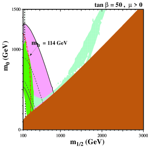
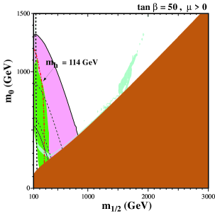
Figure 8: As in Fig. 7 for $\tan\beta=50$.

Another mechanism for extending the allowed CMSSM region to large $m_{\chi}$ is rapid annihilation via a direct-channel pole when $m_{\chi}\sim{1\over 2}m_{A}$ [69, 70]. Since the heavy scalar and pseudoscalar Higgs masses decrease as $\tan\beta$ increases, eventually $2m_{\chi}\simeq m_{A}$ yielding a ‘funnel’ extending to large $m_{1/2}$ and $m_{0}$ at large $\tan\beta$, as seen in the high $\tan\beta$ strips of Fig. 8. As one can see, the impact of the Higgs mass constraint is reduced (relative to the case with $\tan\beta=10$) while that of $b\to s\gamma$ is enhanced.

Shown in Fig. 9 are the WMAP lines[66] of the $(m_{1/2},m_{0})$ plane allowed by the new cosmological constraint $0.094<\Omega_{\chi}h^{2}<0.129$ and the laboratory constraints listed above, for $\mu>0$ and values of $\tan\beta$ from 5 to 55, in steps $\Delta(\tan\beta)=5$. We notice immediately that the strips are considerably narrower than the spacing between them, though any intermediate point in the $(m_{1/2},m_{0})$ plane would be compatible with some intermediate value of $\tan\beta$. The right (left) ends of the strips correspond to the maximal (minimal) allowed values of $m_{1/2}$ and hence $m_{\chi}$. The lower bounds on $m_{1/2}$ are due to the Higgs mass constraint for $\tan\beta\leq 23$, but are determined by the $b\to s\gamma$ constraint for higher values of $\tan\beta$.

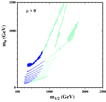
Figure 9: The strips display the regions of the $(m_{1/2},m_{0})$ plane that are compatible with $0.094<\Omega_{\chi}h^{2}<0.129$ and the laboratory constraints for $\mu>0$ and $\tan\beta=5,10,15,20,25,30,35,40,45,50,55$. The parts of the strips compatible with $g_{\mu}-2$ at the 2-$\sigma$ level have darker shading.

Finally, there is one additional region of acceptable relic density known as the focus-point region[71], which is found at very high values of $m_{0}$. An example showing this region is found in Fig. 10, plotted for $\tan\beta=10$, $\mu>0$, and $m_{t}=175$ TeV. As $m_{0}$ is increased, the solution for $\mu$ at low energies as determined by the electroweak symmetry breaking conditions eventually begins to drop. When $\mu\mathrel{\raise 1.29167pt\hbox{$<$\kern-7.5pt\lower 4.30554pt\hbox{$\sim$}}}m_{1/2}$, the composition of the LSP gains a strong Higgsino component and as such the relic density begins to drop precipitously. These effects are both shown in Fig. 11 where the value of $\mu$ and $\Omega h^{2}$ are plotted as a function of $m_{0}$ for fixed $m_{1/2}=300$ GeV and $\tan\beta=10$. As $m_{0}$ is increased further, there are no longer any solutions for $\mu$. This occurs in the shaded region in the upper left corner of Fig. 10.

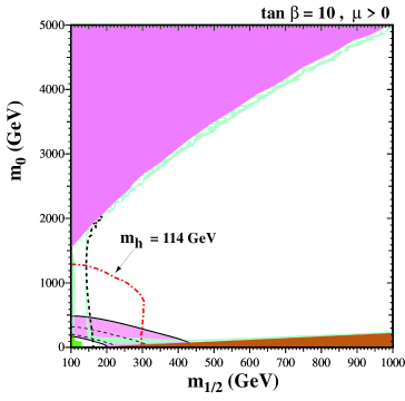
Figure 10: As in Fig. 7a, where the range in $m_{0}$ is extended to 5 TeV. In the shaded region at very high $m_{0}$, there are no solutions for $\mu$ which respect the low energy electroweak symmetry breaking conditions.

Fig. 11 also exemplifies the degree of fine tuning associated with the focus-point region. While the position of the focus-point region in the $m_{0},m_{1/2}$ plane is not overly sensitive to supersymmetric parameters, it is highly sensitive to the top quark Yukawa coupling which contributes to the evolution of $\mu$ [72, 73]. As one can see in the figure, a change in $m_{t}$ of 3 GeV produces a shift of about 2.5 TeV in $m_{0}$. Note that the position of the focus-point region is also highly sensitive to the value of $A_{0}/m_{0}$. In Fig. 11, $A_{0}=0$ was chosen. For $A_{0}/m_{0}=0.5$, the focus point shifts from 2.5 to 4.5 TeV and moves to larger $m_{0}$ as $A_{0}/m_{0}$ is increased.

Figure 11: The value of $\mu$ as a function of $m_{0}$ for fixed $m_{1/2}=300$ GeV and $\tan\beta=10$ for two choices of $m_{t}$ as indicated. The scale on the right gives the value of $\Omega h^{2}$. The curves corresponding to this is scale rise sharply at low $m_{0}$ to values much larger than 1. For $m_{t}=175$ GeV and $m_{0}\approx 2500$ GeV, the value of $\Omega h^{2}$ drops to acceptable values when $\mu$ becomes small. When the $m_{t}=178$ GeV, $\Omega h^{2}$ drops at $m_{0}\approx 5000$ GeV.

4.5 A Likelihood analysis of the CMSSM

In displaying acceptable regions of cosmological density in the $m_{0},m_{1/2}$ plane, it has been assumed that the input parameters are known with perfect accuracy so that the relic density can be calculated precisely. While all of the beyond the standard model parameters are completely unknown and therefore carry no formal uncertainties, standard model parameters such as the top and bottom Yukawa couplings are known but do carry significant uncertainties.

The optimal way to combine the various constraints (both phenomenological and cosmological) is via a likelihood analysis. When performing such an analysis, in addition to the formal experimental errors, it is also essential to take into account theoretical errors, which introduce systematic uncertainties that are frequently non-negligible. Recently, we have preformed an extensive likelihood analysis of the CMSSM[74].

The interpretation of the combined Higgs likelihood, ${L}_{exp}$, in the $(m_{1/2},m_{0})$ plane depends on uncertainties in the theoretical calculation of $m_{h}$. These include the experimental error in $m_{t}$ and (particularly at large $\tan\beta$) $m_{b}$, and theoretical uncertainties associated with higher-order corrections to $m_{h}$. Our default assumptions are that $m_{t}=175\pm 5$ GeV for the pole mass, and $m_{b}=4.25\pm 0.25$ GeV for the running $\overline{MS}$ mass evaluated at $m_{b}$ itself. The theoretical uncertainty in $m_{h}$, $\sigma_{th}$, is dominated by the experimental uncertainties in $m_{t,b}$, which are treated as uncorrelated Gaussian errors:

$${\sigma_{th}}^{2}=\left(\frac{\partial m_{h}}{\partial m_{t}}\right)^{2}\Delta m_{t}^{2}+\left(\frac{\partial m_{h}}{\partial m_{b}}\right)^{2}\Delta m_{b}^{2}\,.$$ (20)

Typically, we find that $(\partial m_{h}/\partial m_{t})\sim 0.5$, so that $\sigma_{th}$ is roughly 2-3 GeV.

The combined experimental likelihood, ${\mathcal{L}}_{exp}$, from direct searches at LEP 2 and a global electroweak fit is then convolved with a theoretical likelihood (taken as a Gaussian) with uncertainty given by $\sigma_{th}$ from (20) above. Thus, we define the total Higgs likelihood function, ${\mathcal{L}}_{h}$, as

$${\mathcal{L}}_{h}(m_{h})={{\mathcal{N}}\over{\sqrt{2\pi}\,\sigma_{th}}}\int dm^{\prime}_{h}\,\,{\mathcal{L}}_{exp}(m^{\prime}_{h})\,\,e^{-(m^{\prime}_{h}-m_{h})^{2}/2\sigma_{th}^{2}}\,,$$ (21)

where ${\mathcal{N}}$ is a factor that normalizes the experimental likelihood distribution. In addition to the Higgs likelihood function, we have included the likelihood function based on $b\to s\gamma$. While the likelihood function based on the measurements of the anomalous magnetic moment of the muon was considered in [74], it will not be discussed here.

Finally, in calculating the likelihood of the CDM density, we take into account the contribution of the uncertainties in $m_{t,b}$. We will see that the theoretical uncertainty plays a very significant role in this analysis. The likelihood for $\Omega h^{2}$ is therefore,

$${\mathcal{L}}_{\Omega h^{2}}=\frac{1}{\sqrt{2\pi}\sigma}e^{-({\Omega h^{2}}^{th}-{\Omega h^{2}}^{exp})^{2}/2\sigma^{2}}\,,$$ (22)

where $\sigma^{2}=\sigma_{exp}^{2}+\sigma_{th}^{2}$, with $\sigma_{exp}$ taken from the WMAP[9] result and $\sigma_{th}^{2}$ from (20), replacing $m_{h}$ by $\Omega h^{2}$.

The total likelihood function is computed by combining all the components described above:

$${\mathcal{L}}_{tot}={\mathcal{L}}_{h}\times{\mathcal{L}}_{bs\gamma}\times{\mathcal{L}}_{\Omega_{\chi}h^{2}}(\times{\mathcal{L}}_{a_{\mu}})$$ (23)

The likelihood function in the CMSSM can be considered a function of two variables, ${\mathcal{L}}_{tot}(m_{1/2},m_{0})$, where $m_{1/2}$ and $m_{0}$ are the unified GUT-scale gaugino and scalar masses respectively.

Using a fully normalized likelihood function ${\mathcal{L}}_{tot}$ obtained by combining both signs of $\mu$ for each value of $\tan\beta$, we can determine the regions in the $(m_{1/2},m_{0})$ planes which correspond to specific CLs as shown in Fig. 12. The darkest (blue), intermediate (red) and lightest (green) shaded regions are, respectively, those where the likelihood is above 68%, above 90%, and above 95%.

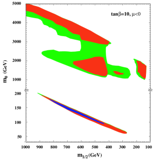
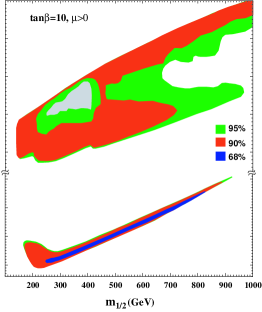
Figure 12: Contours of the likelihood at the 68%, 90% and 95% levels for $\tan\beta=10$, $A_{0}=0$ and $\mu>0$ (left panel) or $\mu<0$ (right panel), calculated using information of $m_{h}$, $b\to s\gamma$ and $\Omega_{CDM}h^{2}$ and the current uncertainties in $m_{t}$ and $m_{b}$.

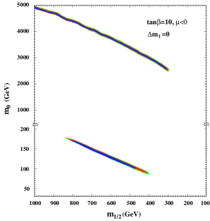
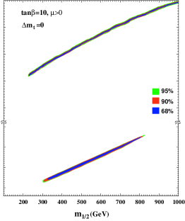
Figure 13: As in Fig. 12 but assuming zero uncertainty in $m_{t}$.

The bulk region is more apparent in the right panel of Fig. 12 for $\mu>0$ than it would be if the experimental error in $m_{t}$ and the theoretical error in $m_{h}$ were neglected. Fig. 13 complements the previous figures by showing the likelihood functions as they would appear if there were no uncertainty in $m_{t}$, keeping the other inputs the same. We see that, in this case, both the coannihilation and focus-point strips rise above the 68% CL.

4.6 Beyond the CMSSM

The results of the CMSSM described in the previous sections are based heavily on the assumptions of universality of the supersymmetry breaking parameters. One of the simplest generalizations of this model relaxes the assumption of universality of the Higgs soft masses and is known as the NUHM[75] In this case, the input parameters include $\mu$ and $m_{A},$ in addition to the standard CMSSM inputs. In order to switch $\mu$ and $m_{A}$ from outputs to inputs, the two soft Higgs masses, $m_{1},m_{2}$ can no longer be set equal to $m_{0}$ and instead are calculated from the electroweak symmetry breaking conditions. The NUHM parameter space was recently analyzed[75] and a sample of the results are shown in Fig. 14.

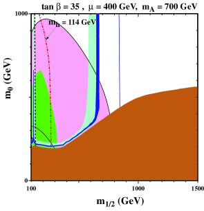
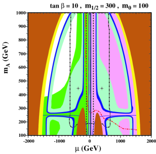
Figure 14: a) The NUHM $(m_{1/2},m_{0})$ plane for $\tan\beta=35$, (a) $\mu=400$ GeV and $m_{A}=700$ GeV b)the NUHM $(\mu,m_{A})$ plane for $\tan\beta=10$, $m_{0}=100$ GeV and $m_{1/2}=300$ GeV, with $A_{0}=0$. The (red) dot-dashed lines are the contours $m_{h}=114$ GeV, and the near-vertical (black) dashed lines are the contours $m_{\chi^{\pm}}=103.5$ GeV. The dark (black) dot-dashed lines indicate the GUT stability constraint. Only the areas inside these curves (small $\mu$) are allowed by this constraint. The light (turquoise) shaded areas are the cosmologically preferred regions with $0.1\leq\Omega_{\chi}h^{2}\leq 0.3$. The darker (blue) portion of this region corresponds to the WMAP densities. The dark (brick red) shaded regions is excluded because the stau is the LSP, and the lighter (yellow) shaded regions is excluded because the LSP is a sneutrino. The medium (green) shaded region is excluded by $b\to s\gamma$. The regions allowed by the $g-2$ constraint are shaded (pink) and bounded by solid black lines. The solid (blue) curves correspond to $m_{\chi}=m_{A}/2$.

In the left panel of Fig. 14, we see a $m_{1/2},m_{0}$ plane with a relative low value of $\mu$. In this case, an allowed region is found when the LSP contains a non-negligible Higgsino component which moderates the relic density independent of $m_{0}$. To the right of this region, the relic density is too small. In the right panel, we see an example of the $m_{A},\mu$ plane. The crosses correspond to CMSSM points. In this single pane, we see examples of acceptable cosmological regions corresponding to the bulk region, co-annihilation region and s-channel annihilation through the Higgs pseudo scalar.

Rather than relax the CMSSM, it is in fact possible to further constrain the model. While the CMSSM models described above are certainly mSUGRA inspired, minimal supergravity models can be argued to be still more predictive. In the simplest version of the theory[76] where supersymmetry is broken in a hidden sector, the universal trilinear soft supersymmetry-breaking terms are $A=(3-\sqrt{3})m_{0}$ and bilinear soft supersymmetry-breaking term is $B=(2-\sqrt{3})m_{0}$, i.e., a special case of a general relation between $B$ and $A$, $B_{0}=A_{0}-m_{0}$.

Given a relation between $B_{0}$ and $A_{0}$, we can no longer use the standard CMSSM boundary conditions, in which $m_{1/2}$, $m_{0}$, $A_{0}$, $\tan\beta$, and $sgn(\mu)$ are input at the GUT scale with $\mu$ and $B$ determined by the electroweak symmetry breaking condition. Now, one is forced to input $B_{0}$ and instead $\tan\beta$ is calculated from the minimization of the Higgs potential[77]. In Fig. 15, the contours of $\tan\beta$ (solid blue lines) in the $(m_{1/2},m_{0})$ planes for two values of ${\hat{A}}=A_{0}/m_{0}$, ${\hat{B}}=B_{0}/m_{0}={\hat{A}}-1$ and the sign of $\mu$ are displayed[77].

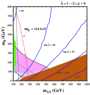
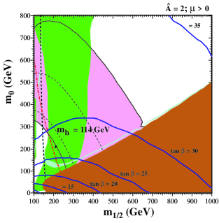
Figure 15: Examples of $(m_{1/2},m_{0})$ planes with contours of $\tan\beta$ superposed, for $\mu>0$ and (a) the simplest Polonyi model with ${\hat{A}}=3-\sqrt{3},{\hat{B}}={\hat{A}}-1$ and (b) ${\hat{A}}=2.0,{\hat{B}}={\hat{A}}-1$. In each panel, we show the regions excluded by the LEP lower limits on MSSM particles, those ruled out by $b\to s\gamma$ decay (medium green shading), and those excluded because the LSP would be charged (dark red shading). The region favoured by the WMAP range has light turquoise shading. The region suggested by $g_{\mu}-2$ is medium (pink) shaded.

In panel (a) of Fig. 15, we see that the Higgs constraint combined with the relic density requires $\tan\beta\mathrel{\raise 1.29167pt\hbox{$>$\kern-7.5pt\lower 4.30554pt\hbox{$\sim$}}}11$, whilst the relic density also enforces $\tan\beta\mathrel{\raise 1.29167pt\hbox{$<$\kern-7.5pt\lower 4.30554pt\hbox{$\sim$}}}20$. For a given point in the $m_{1/2}-m_{0}$ plane, the calculated value of $\tan\beta$ increases as ${\hat{A}}$ increases. This is seen in panel (b) of Fig. 15, when ${\hat{A}}=2.0$, close to its maximal value for $\mu>0$, the $\tan\beta$ contours turn over towards smaller $m_{1/2}$, and only relatively large values $25\mathrel{\raise 1.29167pt\hbox{$<$\kern-7.5pt\lower 4.30554pt\hbox{$\sim$}}}\tan\beta\mathrel{\raise 1.29167pt\hbox{$<$\kern-7.5pt\lower 4.30554pt\hbox{$\sim$}}}35$ are allowed by the $b\to s\gamma$ and $\Omega_{CDM}h^{2}$ constraints, respectively. For any given value of ${\hat{A}}$, there is only a relatively narrow range allowed for $\tan\beta$.

4.7 Detectability

Direct detection techniques rely on an ample neutralino-nucleon scattering cross-section. In Fig. 16, we display the allowed ranges of the spin-independent cross sections in the NUHM when we sample randomly $\tan\beta$ as well as the other NUHM parameters[78]. The raggedness of the boundaries of the shaded regions reflects the finite sample size. The dark shaded regions includes all sample points after the constraints discussed above (including the relic density constraint) have been applied. In a random sample, one often hits points which are are perfectly acceptable at low energy scales but when the parameters are run to high energies approaching the GUT scale, one or several of the sparticles mass squared runs negative. This has been referred to as the GUT constraint here. The medium shaded region embodies those points after the GUT constraint has been applied. After incorporating all the cuts, including that motivated by $g_{\mu}-2$, we find that the light shaded region where the scalar cross section has the range $10^{-6}$ pb $\mathrel{\raise 1.29167pt\hbox{$>$\kern-7.5pt\lower 4.30554pt\hbox{$\sim$}}}\sigma_{SI}\mathrel{\raise 1.29167pt\hbox{$>$\kern-7.5pt\lower 4.30554pt\hbox{$\sim$}}}10^{-10}$ pb, with somewhat larger (smaller) values being possible in exceptional cases.

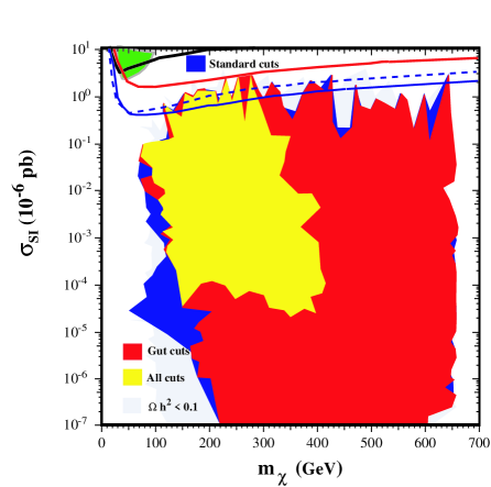
Figure 16: Ranges of the spin-independent cross section in the NUHM. The ranges allowed by the cuts on $\Omega_{\chi}h^{2}$, $m_{h}$ and $b\to s\gamma$ have dark shading, those still allowed by the GUT stability cut have medium shading, and those still allowed after applying all the cuts including $g_{\mu}-2$ have light shading. The pale shaded region corresponds to the extra area of points with low relic densities, whose cross sections have been rescaled appropriately. Also shown are the limits from the CDMS[79] and Edelweiss[80] experiments as well as the recent CDMSII result [81] on the neutralino-proton elastic scattering cross section as a function of the neutralino mass. The CDMSII limit is stronger than the Edelweiss limit which is stronger than the previous CDMS limit at higher $m_{\chi}$. The result reported by DAMA [82] is found in the upper left.

The results from this analysis[78] for the scattering cross section in the NUHM (which by definition includes all CMSSM results) are compared with the previous CDMS[79] and Edelweiss[80] bounds as well as the recent CDMSII results[81] in Fig. 16. While previous experimental sensitivities were not strong enough to probe predictions of the NUHM, the current CDMSII bound has begun to exclude realistic models and it is expected that these bounds improve by a factor of about 20. See ref. [83] for updated direct detection calculations in the MSSM.

5 Big Bang Nucleosynthesis

The standard model[84] of big bang nucleosynthesis (BBN) is based on the relatively simple idea of including an extended nuclear network into a homogeneous and isotropic cosmology. Apart from the input nuclear cross sections, the theory contains only a single parameter, namely the baryon-to-photon ratio, $\eta$. Other factors, such as the uncertainties in reaction rates, and the neutron mean-life can be treated by standard statistical and Monte Carlo techniques[85, 86, 87, 88, 89]. The theory then allows one to make predictions (with well-defined uncertainties) of the abundances of the light elements, D, ${}^{3}{\rm He}$, ${}^{4}{\rm He}$, and ${}^{7}{\rm Li}$.

5.1 Theory

Conditions for the synthesis of the light elements were attained in the early Universe at temperatures $T\mathrel{\raise 1.29167pt\hbox{$>$\kern-7.5pt\lower 4.30554pt\hbox{$\sim$}}}$ 1 MeV. In the early Universe, the energy density was dominated by radiation with

$$\rho={\pi^{2}\over 30}(2+{7\over 2}+{7\over 4}N_{\nu})T^{4}$$ (24)

from the contributions of photons, electrons and positrons, and $N_{\nu}$ neutrino flavors (at higher temperatures, other particle degrees of freedom should be included as well). At these temperatures, weak interaction rates were in equilibrium. In particular, the processes

$$n+e^{+} \leftrightarrow p+{\bar{\nu}_{e}}$$

$$n+\nu_{e} \leftrightarrow p+e^{-}$$

$$n \leftrightarrow p+e^{-}+{\bar{\nu}_{e}}$$ (25)

fix the ratio of number densities of neutrons to protons. At $T\gg 1$ MeV, $(n/p)\simeq 1$.

The weak interactions do not remain in equilibrium at lower temperatures. Freeze-out occurs when the weak interaction rate, $\Gamma_{wk}\sim G_{F}^{2}T^{5}$ falls below the expansion rate which is given by the Hubble parameter, $H\sim\sqrt{G_{N}\rho}\sim T^{2}/M_{P}$, where $M_{P}=1/\sqrt{G_{N}}\simeq 1.2\times 10^{19}$ GeV. The $\beta$-interactions in eq. (25) freeze-out at about 0.8 MeV. As the temperature falls and approaches the point where the weak interaction rates are no longer fast enough to maintain equilibrium, the neutron to proton ratio is given approximately by the Boltzmann factor, $(n/p)\simeq e^{-\Delta m/T}\sim 1/6$, where $\Delta m$ is the neutron-proton mass difference. After freeze-out, free neutron decays drop the ratio slightly to about 1/7 before nucleosynthesis begins.

The nucleosynthesis chain begins with the formation of deuterium by the process, $p+n\rightarrow$ D $+~{}\gamma$. However, because of the large number of photons relative to nucleons, $\eta^{-1}=n_{\gamma}/n_{B}\sim 10^{10}$, deuterium production is delayed past the point where the temperature has fallen below the deuterium binding energy, $E_{B}=2.2$ MeV (the average photon energy in a blackbody is ${\bar{E}}_{\gamma}\simeq 2.7T$). This is because there are many photons in the exponential tail of the photon energy distribution with energies $E>E_{B}$ despite the fact that the temperature or ${\bar{E}}_{\gamma}$ is less than $E_{B}$. The degree to which deuterium production is delayed can be found by comparing the qualitative expressions for the deuterium production and destruction rates,

$$\Gamma_{p} \approx n_{B}\sigma v$$ (26)

$$\Gamma_{d} \approx n_{\gamma}\sigma ve^{-E_{B}/T}$$

When the quantity $\eta^{-1}{\rm exp}(-E_{B}/T)\sim 1$, the rate for deuterium destruction (D $+~{}\gamma\rightarrow p+n$) finally falls below the deuterium production rate and the nuclear chain begins at a temperature $T\sim 0.1MeV$.

The dominant product of big bang nucleosynthesis is ${}^{4}{\rm He}$ and its abundance is very sensitive to the $(n/p)$ ratio

$$Y_{p}={2(n/p)\over\left[1+(n/p)\right]}\approx 0.25$$ (27)

i.e., an abundance of close to 25% by mass. Lesser amounts of the other light elements are produced: D and ${}^{3}{\rm He}$ at the level of about $10^{-5}$ by number, and ${}^{7}{\rm Li}$ at the level of $10^{-10}$ by number.

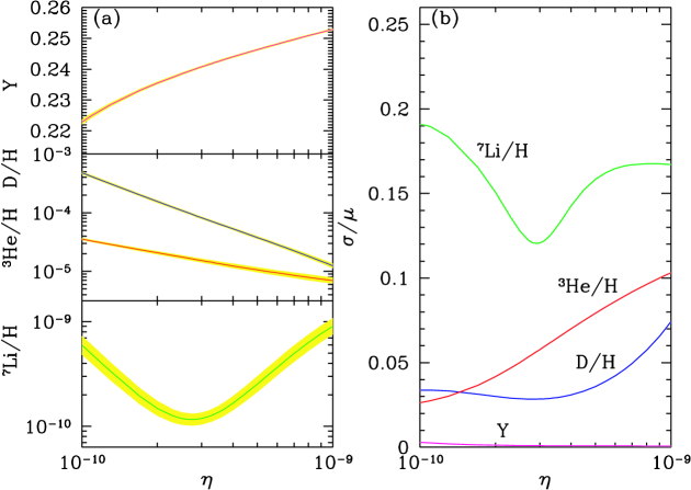
Figure 17: The light element abundances from big bang nucleosynthesis as a function of $\eta_{10}$.

Recently the input nuclear data have been carefully reassessed[87, 88, 89, 90, 91], leading to improved precision in the abundance predictions. The NACRE collaboration presented an updated nuclear compilation [90]. For example, notable improvements include a reduction in the uncertainty in the rate for ${}^{3}{\rm He}$$(n,p)$T from 10% [86] to 3.5% and for T$(\alpha,\gamma)$${}^{7}{\rm Li}$ from $\sim 23-30\%$ [86] to $\sim 4\%$. Since then, new data and techniques have become available, motivating new compilations. Within the last year, several new BBN compilations have been presented[92, 93, 94].

The resulting elemental abundances predicted by standard BBN are shown in Fig. 17 as a function of $\eta$ [88]. The left plot shows the abundance of ${}^{4}{\rm He}$ by mass, $Y$, and the abundances of the other three isotopes by number. The curves indicate the central predictions from BBN, while the bands correspond to the uncertainty in the predicted abundances. This theoretical uncertainty is shown explicitly in the right panel as a function of $\eta$.

In the standard model with $N_{\nu}=3$, the only free parameter is the density of baryons which sets the rates of the strong reactions. Thus, any abundance measurement determines $\eta$, while additional measurements overconstrain the theory and thereby provide a consistency check. BBN has thus historically been the premier means of determining the cosmic baryon density. With the increased precision of microwave background anisotropy measurements, it is now possible to use the the CMB to independently determine the baryon density. The WMAP value for $\Omega_{B}h^{2}=0.0224$ translates into

$$\eta_{10}=6.14\pm 0.25$$ (28)

With $\eta$ fixed by the CMB, precision comparisons to the observations can now be attempted[95].

5.2 Light Element Observations and Comparison with Theory

BBN theory predicts the universal abundances of D, ${}^{3}{\rm He}$, ${}^{4}{\rm He}$, and ${}^{7}{\rm Li}$, which are essentially determined by $t\sim 180$ s. Abundances are however observed at much later epochs, after stellar nucleosynthesis has commenced. The ejected remains of this stellar processing can alter the light element abundances from their primordial values, and produce heavy elements such as C, N, O, and Fe (“metals”). Thus one seeks astrophysical sites with low metal abundances, in order to measure light element abundances which are closer to primordial. For all of the light elements, systematic errors are an important and often dominant limitation to the precision of derived primordial abundances.

5.2.1 D/H

In recent years, high-resolution spectra have revealed the presence of D in high-redshift, low-metallicity quasar absorption systems (QAS), via its isotope-shifted Lyman-$\alpha$ absorption. These are the first measurements of light element abundances at cosmological distances. It is believed that there are no astrophysical sources of deuterium[96], so any measurement of D/H provides a lower limit to primordial D/H and thus an upper limit on $\eta$; for example, the local interstellar value of D/H=$(1.5\pm 0.1)\times 10^{-5}$ citelin requires that $\eta_{10}\leq 9$. In fact, local interstellar D may have been depleted by a factor of 2 or more due to stellar processing; however, for the high-redshift systems, conventional models of galactic nucleosynthesis (chemical evolution) do not predict significant D/H depletion[98].

The five most precise observations of deuterium[99, 100, 101, 102] in QAS give D/H = $(2.78\pm 0.29)\times 10^{-5}$, where the error is statistical only. These are shown in Fig. 18 along with some other recent measurements[103, 104, 105]. Inspection of the data shown in the figure clearly indicates the need for concern over systematic errors. We thus conservatively bracket the observed values with a range D/H = $2-5\times 10^{-5}$ which corresponds to a range in $\eta_{10}$ of 4 – 8 which easily brackets the CMB determined value.

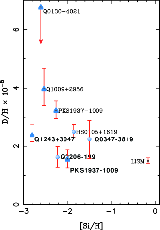
Figure 18: D/H abundances shown as a function of [Si/H].

Using the WMAP value for the baryon density (28) the primordial D/H abundance is predicted to be[88, 92]:

$$({\rm D/H})_{p}=2.55^{+0.21}_{-0.20}\times 10^{-5}$$ (29)

As one can see, this value is in very good agreement with the observational value.

5.3 ${}^{4}{\rm He}$

We observe ${}^{4}{\rm He}$ in clouds of ionized hydrogen (HII regions), the most metal-poor of which are in dwarf galaxies. There is now a large body of data on ${}^{4}{\rm He}$ and CNO in these systems[106]. Of the modern ${}^{4}{\rm He}$ determinations, the work of Pagel et al.[107] established the analysis techniques that were soon to follow[108]. Their value of $Y_{p}$ $=$ 0.228 $\pm$ 0.005 was significantly lower than that of a sample of 45 low metallicity HII regions, observed and analyzed in a uniform manner[106], with a derived value of $Y_{p}$ $=$ 0.244 $\pm$ 0.002. An analysis based on the combined available data as well as unpublished data yielded an intermediate value of 0.238 $\pm$ 0.002 with an estimated systematic uncertainty of 0.005 [109]. An extended data set including 89 HII regions obtained $Y_{p}$ $=$ 0.2429 $\pm$ 0.0009 [110]. However, the recommended value is based on the much smaller subset of 7 HII regions, finding $Y_{p}$ $=$ 0.2421 $\pm$ 0.0021.

${}^{4}{\rm He}$ abundance determinations depend on a number of physical parameters associated with the HII region in addition to the overall intensity of the He emission line. These include, the temperature, electron density, optical depth and degree of underlying absorption. A self-consistent analysis may use multiple ${}^{4}{\rm He}$ emission lines to determine the He abundance, the electron density and the optical depth. In [106], five He lines were used, underlying He absorption was assumed to be negligible and used temperatures based on OIII data.

The question of systematic uncertainties was addressed in some detail in [111]. It was shown that there exist severe degeneracies inherent in the self-consistent method, particularly when the effects of underlying absorption are taken into account. The results of a Monte-Carlo reanalysis[112] of NCG 346[113] is shown in Fig. 19. In the left panel, solutions for the ${}^{4}{\rm He}$ abundance and electron density are shown (symbols are described in the caption). In the right panel, a similar plot with the ${}^{4}{\rm He}$ abundance and the equivalent width for underlying absorption is shown. As one can see, solutions with no absorption and high density are often indistinguishable (i.e., in a statistical sense they are equally well represented by the data) from solutions with underlying absorption and a lower density. In the latter case, the He abundance is systematically higher. These degeneracies are markedly apparent when the data is analyzed using Monte-Carlo methods which generate statistically viable representations of the observations as shown in Fig. 19. When this is done, not only are the He abundances found to be higher, but the uncertainties are also found to be significantly larger than in a direct self-consistent approach.

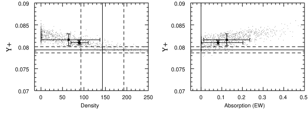
Figure 19: Results of modeling of 6 He I line observations of NGC 346[113]. The solid lines show the original derived values and the dashed lines show the 1 $\sigma$ errors on those values. The solid circles (with error bars) show the results of the $\chi^{2}$ minimization solution (with calculated errors)[112]. The small points show the results of Monte Carlo realizations of the original input spectrum. The solid squares (with error bars) show the means and dispersions of the output values for the $\chi^{2}$ minimization solutions of the Monte Carlo realizations.

Recently a careful study of the systematic uncertainties in ${}^{4}{\rm He}$, particularly the role of underlying absorption has been performed using a subset of the highest quality from the data of Izotov and Thuan[106]. All of the physical parameters listed above including the ${}^{4}{\rm He}$ abundance were determined self-consistently with Monte Carlo methods[111]. Note that the ${}^{4}{\rm He}$ abundances are systematically higher, and the uncertainties are several times larger than quoted in [106]. In fact this study has shown that the determined value of $Y_{p}$ is highly sensitive to the method of analysis used. The result is shown in Fig. 20 together with a comparison of the previous result. The extrapolated ${}^{4}{\rm He}$ abundance was determined to be $Y_{p}=0.2495\pm 0.0092$. The value of $\eta$ corresponding to this abundance is $\eta_{10}=6.9^{+11.8}_{-4.0}$ and clearly overlaps with $\eta_{CMB}$. Conservatively, it would be difficult at this time to exclude any value of $Y_{p}$ inside the range 0.232 – 0.258.

At the WMAP value for $\eta$, the ${}^{4}{\rm He}$ abundance is predicted to be[88, 92]:

$$Y_{p}=0.2485\pm 0.0005$$ (30)

This value is considerably higher than any prior determination of the primordial ${}^{4}{\rm He}$ abundance, it is in excellent agreement with the most recent analysis of the ${}^{4}{\rm He}$ abundance[112]. Note also that the large uncertainty ascribed to this value indicates that the while ${}^{4}{\rm He}$ is certainly consistent with the WMAP determination of the baryon density, it does not provide for a highly discriminatory test of the theory at this time.

Figure 20: A comparison of the results for the best targets[106] and a re-analysis of the spectra for those targets[112].

5.4 ${}^{7}{\rm Li}$/H

The systems best suited for Li observations are metal-poor halo stars in our Galaxy. Observations have long shown[114] that Li does not vary significantly in Pop II stars with metallicities $\mathrel{\raise 1.29167pt\hbox{$<$\kern-7.5pt\lower 4.30554pt\hbox{$\sim$}}}1/30$ of solar — the “Spite plateau”. Recent precision data suggest a small but significant correlation between Li and Fe [115] which can be understood as the result of Li production from Galactic cosmic rays[116]. Extrapolating to zero metallicity one arrives at a primordial value[117] ${\rm Li/H}|_{p}=(1.23^{+0.34}_{-0.16})\times 10^{-10}$.

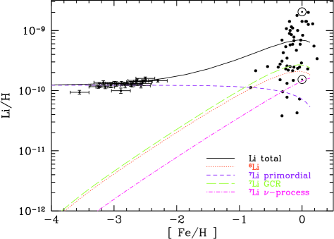
Figure 21: Contributions to the total predicted lithium abundance from the adopted GCE model of [118], compared with low metallicity stars and a sample of high metallicity stars. The solid curve is the sum of all components.

Figure 21 shows the different Li components for a model with (${}^{7}{\rm Li}$/H)${}_{p}=1.23\times 10^{-10}$. The linear slope produced by the model is independent of the input primordial value. The model of ref. [118] includes in addition to primordial ${}^{7}{\rm Li}$, lithium produced in galactic cosmic ray nucleosynthesis (primarily $\alpha+\alpha$ fusion), and ${}^{7}{\rm Li}$ produced by the $\nu$-process during type II supernovae. As one can see, these processes are not sufficient to reproduce the population I abundance of ${}^{7}{\rm Li}$, and additional production sources are needed.

Recent data[119] with temperatures based on H$\alpha$ lines (considered to give systematically high temperatures) yields ${}^{7}{\rm Li}$/H = $(2.19\pm 0.28)\times 10^{-10}$. These results are based on a globular cluster sample (NGC 6397). This result is consistent with previous Li measurements of the same cluster which gave ${}^{7}{\rm Li}$/H = $(1.91\pm 0.44)\times 10^{-10}$ [120] and ${}^{7}{\rm Li}$/H = $(1.69\pm 0.27)\times 10^{-10}$ [121]. A related study (also of globular cluster stars) gives ${}^{7}{\rm Li}$/H = $(2.29\pm 0.94)\times 10^{-10}$ [122].

The ${}^{7}{\rm Li}$ abundance based on the WMAP baryon density is predicted to be[88, 92]:

$${\rm\mbox{${}^{7}{\rm Li}$}/H}=4.26^{+0.73}_{-0.60}\times 10^{-10}$$ (31)

This value is in clear contradiction with most estimates of the primordial Li abundance. It is a factor of $\sim 3$ higher than the value observed in most halo stars, and just about 0.2 dex over the globular cluster value.

5.5 Concordance

In Fig. 22, we show the direct comparison between the BBN predicted abundances given in eqs. (29), (30), and (31), using the WMAP value of $\eta_{10}=6.25\pm 0.25$ with the observations[123]. As one can see, there is very good agreement between theory and observation for both D/H and ${}^{4}{\rm He}$. Of course, in the case of ${}^{4}{\rm He}$, concordance is almost guaranteed by the large errors associated to the observed abundance. In contrast, as was just noted above, there is a marked discrepancy in the case of ${}^{7}{\rm Li}$.

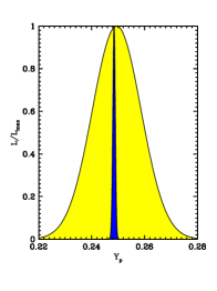
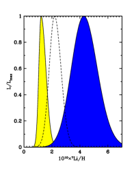
Figure 22: Primordial light element abundances as predicted by BBN and WMAP (dark shaded regions)[123]. Different observational assessments of primordial abundances are plotted as follows: (a) the light shaded region shows ${\rm D/H}=(2.78\pm 0.29)\times 10^{-5}$; (b) the light shaded region shows $Y_{p}=0.249\pm 0.009$; (c) the light shaded region shows ${}^{7}{\rm Li}$/H = $1.23^{+0.34}_{-0.16}\times 10^{-10}$, while the dashed curve shows ${}^{7}{\rm Li}$/H = $(2.19\pm 0.28)\times 10^{-10}$.

The quoted value for the ${}^{7}{\rm Li}$ abundance assumes that the Li abundance in the stellar sample reflects the initial abundance at the birth of the star. However, an important source of systematic uncertainty comes from the possible depletion of Li over the $\mathrel{\raise 1.29167pt\hbox{$>$\kern-7.5pt\lower 4.30554pt\hbox{$\sim$}}}10$ Gyr age of the Pop II stars. The atmospheric Li abundance will suffer depletion if the outer layers of the stars have been transported deep enough into the interior, and/or mixed with material from the hot interior; this may occur due to convection, rotational mixing, or diffusion. Standard stellar evolution models predict Li depletion factors which are very small ($<$0.05 dex) in very metal-poor turnoff stars[124]. However, there is no reason to believe that such simple models incorporate all effects which lead to depletion such as rotationally-induced mixing and/or diffusion. Current estimates for possible depletion factors are in the range $\sim$ 0.2–0.4 dex [125]. As noted above, this data sample[115] shows a negligible intrinsic spread in Li leading to the conclusion that depletion in these stars is as low as 0.1 dex.

Another important source for potential systematic uncertainty stems from the fact that the Li abundance is not directly observed but rather, inferred from an absorption line strength and a model stellar atmosphere. Its determination depends on a set of physical parameters and a model-dependent analysis of a stellar spectrum. Among these parameters, are the metallicity characterized by the iron abundance (though this is a small effect), the surface gravity which for hot stars can lead to an underestimate of up to 0.09 dex if $\log g$ is overestimated by 0.5, though this effect is negligible in cooler stars. Typical uncertainties in $\log g$ are $\pm 0.1-0.3$. The most important source for error is the surface temperature. Effective-temperature calibrations for stellar atmospheres can differ by up to 150–200 K, with higher temperatures resulting in estimated Li abundances which are higher by $\sim 0.08$ dex per 100 K. Thus accounting for a difference of 0.5 dex between BBN and the observations, would require a serious offset of the stellar parameters. While there has been a recent analysis[126] which does support higher temperatures, the consequences of the higher temperatures on the inferred abundances of related elements such as Be, B, and O observed in the same stars is somewhat negative[127].

Finally a potential source for systematic uncertainty lies in the BBN calculation of the ${}^{7}{\rm Li}$ abundance. As one can see from Fig. 17, the predictions for ${}^{7}{\rm Li}$ carry the largest uncertainty of the 4 light elements which stem from uncertainties in the nuclear rates. The effect of changing the yields of certain BBN reactions was recently considered by Coc et al.[91]. In particular, they concentrated on the set of cross sections which affect ${}^{7}{\rm Li}$ and are poorly determined both experimentally and theoretically. In many cases however, the required change in cross section far exceeded any reasonable uncertainty. Nevertheless, it may be possible that certain cross sections have been poorly determined. In [91], it was found for example, that an increase of either the $\mbox{${}^{7}{\rm Li}$}(d,n)2\mbox{${}^{4}{\rm He}$}$ or $\mbox{${}^{7}{\rm Be}$}(d,p)2\mbox{${}^{4}{\rm He}$}$ reactions by a factor of 100 would reduce the ${}^{7}{\rm Li}$ abundance by a factor of about 3.

The possibility of systematic errors in the $\mbox{${}^{3}{\rm He}$}(\alpha,\gamma)\mbox{${}^{7}{\rm Be}$}$ reaction, which is the only important ${}^{7}{\rm Li}$ production channel in BBN, was considered in detail in [128]. The absolute value of the cross section for this key reaction is known relatively poorly both experimentally and theoretically. However, the agreement between the standard solar model and solar neutrino data thus provides additional constraints on variations in this cross section. Using the standard solar model of Bahcall[129], and recent solar neutrino data[130], one can exclude systematic variations of the magnitude needed to resolve the BBN ${}^{7}{\rm Li}$ problem at the $\mathrel{\raise 1.29167pt\hbox{$>$\kern-7.5pt\lower 4.30554pt\hbox{$\sim$}}}95\%$ CL [128]. Thus the “nuclear fix” to the ${}^{7}{\rm Li}$ BBN problem is unlikely.

Finally, we turn to ${}^{3}{\rm He}$. Here, the only observations available are in the solar system and (high-metallicity) HII regions in our Galaxy[131]. This makes inference of the primordial abundance difficult, a problem compounded by the fact that stellar nucleosynthesis models for ${}^{3}{\rm He}$ are in conflict with observations[132]. Consequently, it is not appropriate to use ${}^{3}{\rm He}$ as a cosmological probe[133]; instead, one might hope to turn the problem around and constrain stellar astrophysics using the predicted primordial ${}^{3}{\rm He}$ abundance[134]. For completeness, we note that the ${}^{3}{\rm He}$ abundance is predicted to be:

$${\rm\mbox{${}^{3}{\rm He}$}/H}=9.28^{+0.55}_{-0.54}\times 10^{-6}$$ (32)

at the WMAP value of $\eta$.

6 Constraints on Decaying Particles and Gravitino Dark Matter from BBN

As an example of constraints on particle properties from BBN, I will concentrate here on life-time and abundance limits on decaying particles as it ties in well with the previous discussion on supersymmetric dark matter. There are of course many other constraints on particle properties which can be derived from BBN, most notably the limit on the number of relativistic degrees of freedom. For a recent update on these limits, see [123].

Because there is good overall agreement between the theoretical predictions of the light element abundances and their observational determination, any departure from the standard model (or either particle physics, cosmology, or BBN) generally leads to serious inconsistencies among the element abundances.

Gravitinos have long been known to be potentially problematic in cosmology[135]. If gravitinos are present with equilibrium number densities, we can write their energy density as

$$\rho_{3/2}=m_{3/2}n_{3/2}=m_{3/2}\left(3\zeta(3)\over\pi^{2}\right)T_{3/2}^{2}$$ (33)

where today one expects that the gravitino temperature $T_{3/2}$ is reduced relative to the photon temperature due to the annihilations of particles dating back to the Planck time[54]. Typically one can expect the gravitino abundance $Y_{3/2}\equiv n_{3/2}/n_{\gamma}\sim(T_{3/2}/T_{\gamma})^{3}\sim 10^{-2}$. Then for $\Omega_{3/2}h^{2}\mathrel{\raise 1.29167pt\hbox{$<$\kern-7.5pt\lower 4.30554pt\hbox{$\sim$}}}1$, we obtain the limit that $m_{3/2}\mathrel{\raise 1.29167pt\hbox{$<$\kern-7.5pt\lower 4.30554pt\hbox{$\sim$}}}1$ keV.

Of course, the above mass limit assumes a stable gravitino, the problem persists however, even if the gravitino decays, since its gravitational decay rate is very slow. Gravitinos decay when their decay rate, $\Gamma_{3/2}\simeq m_{3/2}^{3}/M_{P}^{2}$, becomes comparable to the expansion rate of the Universe (which becomes dominated by the mass density of gravitinos), $H\simeq m_{3/2}^{1/2}T_{3/2}^{3/2}/M_{P}$. Thus decays occur at $T_{d}\simeq m_{3/2}^{5/3}/M_{P}^{2/3}$. After the decay, the Universe is “reheated” to a temperature

$$T_{R}\simeq\rho(T_{d})^{1/4}\simeq m_{3/2}^{3/2}/M_{P}^{1/2}$$ (34)

The Universe must reheat sufficiently so that big bang nucleosynthesis occurs in a standard radiation dominated Universe. For $T_{R}\mathrel{\raise 1.29167pt\hbox{$>$\kern-7.5pt\lower 4.30554pt\hbox{$\sim$}}}1$ MeV, we must require $m_{3/2}\mathrel{\raise 1.29167pt\hbox{$>$\kern-7.5pt\lower 4.30554pt\hbox{$\sim$}}}20$ TeV. This large value threatens the solution of the hierarchy problem.

Inflation could alleviate the gravitino problem by diluting the gravitino abundance to safe levels[136]. If gravitinos satisfy the noninflationary bounds, then their reproduction after inflation is never a problem. For gravitinos with mass of order 100 GeV, dilution without over-regeneration will also solve the problem, but there are several factors one must contend with in order to be cosmologically safe. Gravitino decay products can also upset the successful predictions of Big Bang nucleosynthesis, and decays into LSPs (if R-parity is conserved) can also yield too large a mass density in the now-decoupled LSPs[48]. For unstable gravitinos, the most restrictive bound on their number density comes form the photo-destruction of the light elements produced during nucleosynthesis[137, 138, 139].

Here, we will consider electromagnetic decays, meaning that the decays inject electromagnetic radiation into the early universe. If the decaying particle is abundant enough or massive enough, the injection of electromagnetic radiation can photo-erode the light elements created during primordial nucleosynthesis. The theories we have in mind are generally supersymmetric, in which the gravitino and neutralino are the next-to-lightest and lightest supersymmetric particles, respectively (or vice versa), but the constraints hold for any decay producing electromagnetic radiation. We thus constrain the abundance of such a particle given its mean lifetime $\tau_{X}$. The abundance is constrained through the parameter $\zeta_{X}\equiv m_{X}n_{X}/n_{\gamma}$.

The BBN limits in the $(\zeta_{X},\tau_{X})$ plane is shown in Fig. 23[140]. The constraint placed by the ${}^{4}{\rm He}$ abundance comes from its lower limit, as this scenario destroys ${}^{4}{\rm He}$. Shown are the limits assuming $Y_{min}=0.232$ and 0.227 [138, 123, 140]. The area above these curves are excluded. The deuterium lines correspond to the contours $(1.3\;{\rm or}\;2.2)\times 10^{-5}\;<\;{{\rm D}/{\rm H}}\;<\;5.3\times 10^{-5}$. The first of the lower bounds is the higher line to the left of the cleft, and represents the very conservative lower limit on D/H assumed in [138]. The range 1.3 – 5.3 $\times 10^{-5}$ effectively brackets all recent observations of D/H in quasar absorption systems as discussed above. The second of the lower bounds is the lower line on the left side and represents the 2-$\sigma$ lower limit in the best set of D/H observations. The upper bound is the line to the right of the cleft. A priori, there is also a narrow strip at larger $\zeta_{X}$ and $\tau_{X}$ where the D/H ratio also falls within the acceptable range but this is excluded by the observed ⁴He abundance.

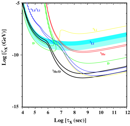
Figure 23: The constraints imposed by the astrophysical observations of ⁴He (red lines), $D/H$ (green lines), ⁶Li (yellow line), ⁶Li/⁷Li (blue lines), ⁷Li (blue band) and ³He (black lines).

The constraint imposed by the ⁶Li abundance is shown [138] as a solid yellow line in Fig. 23. Also shown, as solid blue lines, are two contours representing upper limits on the ⁶Li/⁷Li ratio: ${{}^{6}{\rm Li}/^{7}{\rm Li}}\;<\;0.07\;{\rm or}\;0.15$. The lower number was used in [138] and represented the upper limit available at the time, which was essentially based on multiple observations of a single star. The most recent data[141] includes observations of several stars. The Li isotope ratio for most metal-poor stars in the sample is as high as 0.15, and we display that upper limit here[140]. The main effect of this constraint is to disallow a region in the near-vertical cleft between the upper and lower limits on D/H, as seen in Fig. 23.

The blue shaded band in Fig. 23 corresponds to a ${}^{7}{\rm Li}$ abundance of $0.9\times 10^{-10}\;<\;{{}^{7}{\rm Li}/{\rm H}}\;<\;(2\;{\rm or}\;3)\times 10^{-10},$ with the ⁷Li abundance decreasing as $\zeta_{X}$ increases and the intensity of the shading changing at the intermediate value. In [138], only the lower bound was used due the existing discrepancy between the primordial and observationally determined values. It is apparent that ⁷Li abundances in the lower part of the range are possible only high in the Deuterium cleft, and even then only if one uses the recent and more relaxed limit on the ⁶Li/⁷Li ratio. Values of the ⁷Li abundance in the upper part of the range are possible, however, even if one uses the more stringent constraint on ⁶Li/⁷Li. In this case, the allowed region of parameter space would also extend to lower $\tau_{X}$, if one could tolerate values of D/H between 1.3 and $2.2\times 10^{-5}$.

Finally, we show the impact of the ${}^{3}{\rm He}$ constraint[139, 140]. Since Deuterium is more fragile than ³He, whose abundance is thought to have remained roughly constant since primordial nucleosynthesis when comparing the BBN value to it proto-solar abundance, one would expect, in principle, the ³He/D ratio to have been increased by stellar processing. Since D is totally destroyed in stars, the ratio of ${}^{3}{\rm He}$/D can only increase in time or remain constant if ${}^{3}{\rm He}$ is also completely destroyed in stars. The present or proto-solar value of ³He/D can therefore be used to set an upper limit on the primordial value. Fig. 23 displays the upper limits ${{}^{3}{\rm He}/D}\;<\;1\;{\rm or}\;2$ as solid black lines. Above these contours, the value of ³He/D increases very rapidly, and points high in the Deuterium cleft of Fig. 23 have absurdly high values of ³He/D, exceeding the limit by an order of magnitude or more.

The previous upper limit on $\eta_{X}$ [138] corresponded to the constraint $m_{X}n_{X}/n_{\gamma}<5.0\times 10^{-12}$ GeV for $\tau_{X}=10^{8}$ s. The weaker (stronger) version of the ³He constraint adopted corresponds[140] to

$$m_{X}{n_{X}\over n_{\gamma}}\;<\;2.0(0.8)\times 10^{-12}~{}{\rm GeV}$$ (35)

for $\tau_{X}=10^{8}$ s.

Returning to the case of a decaying gravitino, recall that thermal reactions are estimated to produce an abundance of gravitinos given by [142, 138]:

$${n_{m_{3/2}}\over n_{\gamma}}\;=\;(0.7-2.7)\times 10^{-11}\times\left({T_{R}\over 10^{10}~{}{\rm GeV}}\right).$$ (36)

Assuming that $m_{3/2}=100$ GeV and $\tau_{X}=10^{8}$ s, and imposing the constraints (35), we now find

$$T_{R}\;<\;(0.8-2.8)\times 10^{7}~{}{\rm GeV},\;((0.3-1.1)\times 10^{7}~{}{\rm GeV})$$ (37)

for the weaker (stronger) version of the ³He constraint.

Finally, we consider the possibility that gravitinos are stable and the LSP[143, 144]. In this case, in the CMSSM, the next lightest supersymmetric particle (NSP) is either the neutralino or the stau. In Fig. 24, we fix the ratio of supersymmetric Higgs vacuum expectation values $\tan\beta=10$ (left panel), and $\tan\beta=57$ (right panel), and assume $m_{3/2}=100$ GeV. In each panel of Fig. 24, we display accelerator, astrophysical and cosmological constraints in the corresponding $(m_{1/2},m_{0})$ planes as discussed above for the CMSSM, concentrating on the regions to the right of the near-vertical black lines, where the gravitino is the LSP. The NSP is the $\tau$ lepton below the (red) dotted line.

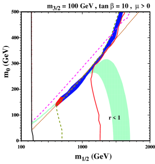
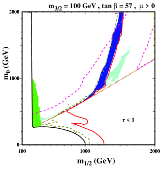
Figure 24: The $(m_{1/2},m_{0})$ planes for $\mu>0$, $m_{3/2}=100$ GeV and (a) $\tan\beta=10$ (b) $\tan\beta=57$. We restrict our attention to the regions between the solid black lines, where the gravitino is the LSP and the NSP lifetime exceeds $10^{4}$ s. In each panel, the near-vertical dashed black (dash-dotted red) line is the constraint $m_{\chi^{\pm}}>104$ GeV ($m_{h}>114$ GeV), the upper (purple) dashed line is the constraint $\Omega_{3/2}h^{2}<0.129$, and the light green shaded region is that where the NSP would have had $0.094\leq\Omega h^{2}\leq 0.129$ if it had not decayed. The solid red (dashed grey-green) line is the region now (previously) allowed by the light-element abundances: $r<1$ as described in the text. The red (blue) shaded region is that where the ${}^{7}{\rm Li}$ abundance could have been improved by NSP decays, but which is now excluded by the ${}^{3}{\rm He}$ (D) constraint.

Below and to the right of the upper (purple) dashed lines, the density of relic gravitinos produced in the decays of other supersymmetric particles is always below the WMAP upper limit: $\Omega_{3/2}h^{2}\leq 0.129$. The code used in [138], when combined with the observational constraints used in [138], yielded the astrophysical constraint represented by the dashed grey-green lines in both panels of Fig. 24 and did not include the constraint due to ${}^{3}{\rm He}$/D. These constraints on the CMSSM parameter plane were computed in [144]. For each point in the $(m_{1/2},m_{0})$, the relic density of either $\chi$ or ${\tilde{\tau}}$ is computed and $\zeta_{X}$ is determined using $\Omega_{X}h^{2}=3.9\times 10^{7}$ GeV $\zeta_{X}$. When $X={\tilde{\tau}}$, $\zeta_{X}$ is reduced by a factor of 0.3, as only 30% of stau decays result in electromagnetic showers which affect the element abundances at these lifetimes. In addition, at each point, the lifetime of the NSP is computed. Then for each $\tau_{X}$, the limit on $\zeta_{X}$ is found from the results shown in Fig. 23. The region to the right of this curve where $r=\zeta_{X}/\zeta_{X}^{limit}<1$ is allowed.

The astrophysical constraints obtained with the newer abundance limits[140] yields the solid red lines in Fig. 24. The examples where $\tau_{X}$ and $\zeta_{X}$ for the NSP decays fall within the ranges shown by the blue band of Fig. 23, and hence are suitable for modifying the ⁷Li abundance[145, 146], are shown as red and blue shaded regions in each panel of Fig. 24. If we had been able to allow a Deuterium abundance as low as D/H $\sim(1-2)\times 10^{-5}$, the blue shaded region would have been able to resolve the Li discrepancy in the context of the CMSSM with gravitino dark matter. The blue region that we now regard as excluded by the lower limit on D/H, which is stronger than that used in [138], extends to large $m_{1/2}$. The red shaded region, which is consistent even with this limit on D/H, but yields very large ³He/D. Fig. 24 show as solid red lines the additional restrictions these constraints impose on the $(m_{1/2},m_{0})$ planes[140].

7 The variation of fundamental constants

There has been considerable interest of late in the possible variation of the fundamental constants. The construction of theories with variable “constants” is straightforward. Consider for example a gravitational Lagrangian which contains the term

$${\mathcal{L}}\sim\phi R,$$ (38)

where $\phi$ is some scalar field and $R$ is the Einstein curvature scalar. The gravitational constant is determined if the dynamics of the theory fix the expectation value of the scalar field so that

$$G_{N}={1\over 16\pi\langle\phi\rangle}.$$ (39)

Similarly a coupling in the Lagrangian of a scalar to the Maxwell term $F^{2}$, fixes the fine-structure constant

$${\mathcal{L}}\sim\phi F^{2},\qquad\alpha={1\over 16\pi\langle\phi\rangle}.$$ (40)

Indeed, gravitational theories of the Jordan-Brans-Dicke type do contain the possibility for a time-varying gravitational constant. However, these theories can always be re-expressed such that $G_{N}$ is fixed and other mass scales in the theory become time dependent (i.e., dependent on the scalar field). For example, the JBD action can be written as

$$S=\int d^{4}x\sqrt{g}\left[\phi R-{\omega\over\phi}\partial_{\mu}\phi\partial^{\mu}\phi+\Lambda+{\mathcal{L}}_{m}(\psi_{matter},g_{\mu\nu})\right],$$ (41)

where $\omega$ is a number which characterizes the degree of departure from general relativity (GR is recovered as $\omega\to\infty$), $\Lambda$ is the cosmological constant, and the matter action for electromagnetism and a single massive fermion can be written as

$${\mathcal{L}}_{m}=-{1\over 4e^{2}}F^{2}-{\overline{\Psi}}\not\!\!D\Psi-m{\overline{\Psi}}\Psi.$$ (42)

Written this way, if the scalar field $\phi$ evolves, then $G_{N}$ does as well. In another conformal frame, the JBD action can be rewritten as

$$S=\int d^{4}x\sqrt{\overline{g}}\left[{\overline{R}}-(\omega+{3\over 2}){(\partial_{\mu}\phi)^{2}\over\phi^{2}}-{{\overline{\Psi}}\not\!\!D\Psi\over\phi^{3/2}}-{m{\overline{\Psi}\Psi}\over\phi^{2}}-{1\over 4e^{2}}F^{2}+{\Lambda\over\phi^{2}}\right].$$ (43)

In this frame, Newton’s constant is constant, but the fermion mass (after $\Psi$ is rescaled) varies as $\phi^{-1/2}$ and the cosmological constant varies as $1/\phi^{2}$. The physics described by either of these two actions is identical and the two frames can not be distinguished as the measurable dimensionless quantity $Gm^{2}\propto\phi^{-1}$ in both frames. While the fine-structure constant remains constant in this construction, it is straight forward to consider theories where it is not. In what follows, I will restrict attention to variations in the fine-structure constant.

In any unified theory in which the gauge fields have a common origin, variations in the fine structure constant will be accompanied by similar variations in the other gauge couplings[147] (see also, [148]). In other words, variations of the gauge coupling at the unified scale will induce variations in all of the gauge couplings at the low energy scale.

It is easy to see that the running of the strong coupling constant has dramatic consequences for the low energy hadronic parameters, including the masses of nucleons[147]. Indeed the masses are determined by the QCD scale, $\Lambda$, which is related to the ultraviolet scale, $M_{UV}$, by dimensional transmutation:

$$\alpha_{s}(M_{UV}^{2})\equiv{g_{s}^{2}(M_{UV}^{2})\over 4\pi}={4\pi\over b_{3}\ln(M_{UV}^{2}/\Lambda^{2})},$$ (44)

where $b_{3}$ is a usual renormalization group coefficient that depends on the number of massless degrees of freedom, running in the loop. Clearly, changes in $g_{s}$ will induce (exponentially) large changes in $\Lambda$:

$${\Delta\Lambda\over\Lambda}={2\pi\over 9\alpha_{s}(M_{UV})}{\Delta\alpha_{s}(M_{UV})\over\alpha_{s}(M_{UV})}\gg{\Delta\alpha_{s}(M_{UV})\over\alpha_{s}(M_{UV})},$$ (45)

where for illustrative purposes we took the beta function of QCD with three fermions. On the other hand, the electromagnetic coupling $\alpha$ never experiences significant running from $M_{UV}$ to $\Lambda$ and thus $\Delta\Lambda/\Lambda\gg\Delta\alpha/\alpha$. A more elaborate treatment of the renormalization group equations above $M_{Z}$ [149] leads to the result that is in perfect agreement with [147]:

$${\Delta\Lambda\over\Lambda}\simeq 30{\Delta\alpha\over\alpha}.$$ (46)

In addition, we expect that not only the gauge couplings will vary, but all Yukawa couplings are expected to vary as well. In [147], the string motivated dependence was found to be

$${\Delta h\over h}={\Delta\alpha_{U}\over\alpha_{U}}$$ (47)

where $\alpha_{U}$ is the gauge coupling at the unification scale and $h$ is the Yukawa coupling at the same scale. However in theories in which the electroweak scale is derived by dimensional transmutation, changes in the Yukawa couplings (particularly the top Yukawa) leads to exponentially large changes in the Higgs vev. In such theories, the Higgs expectation value corresponds to the renormalization point and is given qualitatively by

$$v\sim M_{P}\exp(-2\pi c/\alpha_{t})$$ (48)

where $c$ is a constant of order 1, and $\alpha_{t}=h_{t}^{2}/4\pi$. Thus small changes in $h_{t}$ will induce large changes in $v$. For $c\sim h_{t}\sim 1$,

$${\Delta v\over v}\sim 80{\Delta\alpha_{U}\over\alpha_{U}}$$ (49)

This dependence gets translated into a variation in all low energy particle masses. In short, once we allow $\alpha$ to vary, virtually all masses and couplings are expected to vary as well, typically much more strongly than the variation induced by the Coulomb interaction alone. Unfortunately, it is very hard to make a quantitative prediction for $\Delta v/v$ simply because we do not know exactly how the dimensional transmutation happens in the Higgs sector, and the answer will depend, for example, on such things as the dilaton dependence of the supersymmetry breaking parameters. This uncertainty is characterized in Eq. (48) by the parameter $c$. For the purpose of the present discussion it is reasonable to assume that $\Delta v/v$ is comparable but not exactly equal to $\Delta\Lambda/\Lambda$. That is, although they are both $O(10-100)\Delta\alpha/\alpha$, their difference $|\Delta\Lambda/\Lambda-\Delta v/v|$ is of the same order of magnitude which we will take as $\sim 50\Delta\alpha/\alpha$.

Much of the recent excitement over the possibility of a time variation in the fine structure constant stems from a series of recent observations of quasar absorption systems and a detailed fit of positions of the absorption lines for several heavy elements using the “many-multiplet” method[150, 151]. A related though less sensitive method for testing the variability of $\alpha$, is the alkali doublet method, which neatly describes the physics involved.

Absorption clouds are prevalent along the lines of sight towards distant, high redshift quasars. As such, the quasar acts as a bright source, and the absorption features seen in these clouds reflect their chemical abundances. Consider an absorption feature in a doublet system involving for example, $S_{1/2}\to P_{3/2}$ and $S_{1/2}\to P_{1/2}$ transitions. While the overall wavelength position of the doublet is a measure of the redshift of the absorption cloud, the separation of the two lines is a measure of the fine structure constant. This is easily seen by recalling the energy splitting due to the spin-orbit coupling,

$$\Delta E\sim{e^{2}\over m^{2}r^{3}}S\cdot L\sim me^{8},\qquad{\Delta E\over E}\sim e^{4}\sim\alpha^{2}.$$ (50)

Since the line splitting $\Delta\lambda/\lambda\sim\Delta E/E$, the relative change in the line splitting is directly proportional to $\Delta\alpha/\alpha$. The many multiplet method compares transitions from different multiplets and different atoms and utilizes the effects of relativistic corrections on the spectra. The alkali doublet method[152] has been applied to quasar absorption spectra, but the sensitivity of the method only limits the variation in $\alpha$ within an of order $10^{-5}$. Similarly, at present, considerations based on OIII emission line systems[153] are also only able to set limits on the variation of $\alpha$ at the level of $10^{-4}$.

In contrast, the many multiplet method based on the relativistic corrections to atomic transitions using several transition lines from several elemental species allows for sensitivities which approach the level of $10^{-6}$ [150, 151, 154]. This method compares the line shifts of elements which are particularly sensitive to changes in $\alpha$ with those that are not. At relatively low redshift ($z<1.8$), the method relies on the comparison of Fe lines to Mg lines. At higher redshift, the comparison is mainly between Fe and Si. At all redshifts, other elemental transitions are also included in the analysis. Indeed, when this method is applied to a set of Keck/Hires data, a statistically significant trend for a variation in $\alpha$ was reported: $\Delta\alpha/\alpha=(-0.54\pm 0.12)\times 10^{-5}$ over a redshift range $0.5\mathrel{\raise 1.29167pt\hbox{$<$\kern-7.5pt\lower 4.30554pt\hbox{$\sim$}}}z\mathrel{\raise 1.29167pt\hbox{$<$\kern-7.5pt\lower 4.30554pt\hbox{$\sim$}}}3.0$. The minus sign indicates a smaller value of $\alpha$ in the past.

More recent observations taken at VLT/UVES using the many multiplet method have not been able to duplicate the previous result[154, 155]. The use of Fe lines in [155] on a single absorber found $\Delta\alpha/\alpha=(0.01\pm 0.17)\times 10^{-5}$. However, since the previous result relied on a statistical average of over 100 absorbers, it is not clear that these two results are in contradiction. In [154], the use of Mg and Fe lines in a set of 23 high signal-to-noise systems yielded the result $\Delta\alpha/\alpha=(-0.06\pm 0.06)\times 10^{-5}$ and therefore represents a more significant disagreement and can be used to set very stringent limits on the possible variation in $\alpha$.

There exist various sensitive experimental checks that constrain the variation of coupling constants (see e.g., [156]). Limits can be derived from cosmology (from both big bang nucleosynthesis and the microwave background), the Oklo reactor, long-lived isotopes found in meteoritic samples, and atomic clock measurements.

The most far-reaching limit (in time) on the variation of $\alpha$ comes from BBN. The limit is primarily due to the limit on ${}^{4}{\rm He}$. Changes in the fine structure constant affect directly the neutron-proton mass difference which can be expressed as $\Delta m_{N}\sim a\alpha\Lambda_{QCD}+bv$, where $\Lambda_{QCD}\sim{\mathcal{O}}(100)$ MeV is the mass scale associated with strong interactions, $v\sim{\mathcal{O}}(100)$ GeV determines the weak scale, and $a$ and $b$ are numbers which fix the final contribution to $\Delta m_{N}$ to be $-0.8$ MeV and 2.1 MeV, respectively. From the previous discussion on BBN, changes in $\alpha$ directly induce changes in $\Delta m_{N}$, which affects the neutron to proton ratio. The relatively good agreement between theory and observation, $|\Delta Y/Y|\mathrel{\raise 1.29167pt\hbox{$<$\kern-7.5pt\lower 4.30554pt\hbox{$\sim$}}}3.5\%$ allows one to set a limit $|\Delta\alpha/\alpha|\mathrel{\raise 1.29167pt\hbox{$<$\kern-7.5pt\lower 4.30554pt\hbox{$\sim$}}}0.06$ ($\Delta Y/Y$ scales with $\Delta\alpha/\alpha$) [157, 147, 123]. Since this limit is applied over the age of the Universe, we obtain a limit on the rate of change $|\dot{\alpha}/\alpha|\mathrel{\raise 1.29167pt\hbox{$<$\kern-7.5pt\lower 4.30554pt\hbox{$\sim$}}}4\times 10^{-12}$ yr^-1 over the last 13 Gyr. When coupled variations of the couplings are considered, the above bound is improved by about 2 orders of magnitude to ${\Delta\alpha/\alpha}\mathrel{\raise 1.29167pt\hbox{$<$\kern-7.5pt\lower 4.30554pt\hbox{$\sim$}}}10^{-4}$ as confirmed in a numerical calculation[158].

One can also derive cosmological bounds based on the microwave background. Changes in the fine-structure constant lead directly to changes in the hydrogen binding energy, $E_{b}$. As the Universe expands, its radiation cools to a temperature, $T_{dec}$, at which protons and electrons can combine to form neutral hydrogen atoms, allowing the photons to decouple and free stream. Measurements of the microwave background can determine this temperature to reasonably high accuracy (a few percent)[9]. At decoupling $\eta^{-1}\exp(-E_{b}/T_{dec})\sim 1$. Thus, changes in $\alpha$ of at most a few percent can be tolerated over the time scale associated with decoupling (a redshift of $z\sim 1100$)[159].

Interesting constraints on the variation of $\alpha$ can be obtained from the Oklo phenomenon concerning the operation of a natural reactor in a rich uranium deposit in Gabon approximately two billion years ago. The observed isotopic abundance distribution at Oklo can be related to the cross section for neutron capture on ¹⁴⁹Sm [160]. This cross section depends sensitively on the neutron resonance energy $E_{r}$ for radiative capture by ¹⁴⁹Sm into an excited state of ¹⁵⁰Sm. The observed isotopic ratios only allow a small shift of $|\Delta E_{r}|\mathrel{\raise 1.29167pt\hbox{$<$\kern-7.5pt\lower 4.30554pt\hbox{$\sim$}}}E_{r}$ from the present value of $E_{r}=0.0973$ eV. This then constrains the possible variations in the energy difference between the excited state of ¹⁵⁰Sm and the ground state of ¹⁴⁹Sm over the last two billion years. A contribution to this energy difference comes from the Coulomb energy $E_{C}=(3/5)(e^{2}/r_{0})Z^{2}/A^{1/3}$ ($r_{0}=1.2$ fm) for a nucleus with $Z$ protons and $(A-Z)$ neutrons. This contribution clearly scales with $\alpha$ and is $E_{C}({{}^{150}{\rm Sm}})-E_{C}({{}^{149}{\rm Sm}})=1.16(\alpha/\alpha_{0})$ MeV, where $\alpha_{0}$ is the present value of $\alpha$. Considering the time variation of $\alpha$ alone, $|\Delta E_{r}|\sim 1.16|\Delta\alpha/\alpha|$ MeV and a limit $|\Delta\alpha/\alpha|\mathrel{\raise 1.29167pt\hbox{$<$\kern-7.5pt\lower 4.30554pt\hbox{$\sim$}}}10^{-7}$ can be obtained[160]. However, if all fundamental couplings are allowed to vary interdependently, a much more stringent limit $|\Delta\alpha/\alpha|<(1-5)\times 10^{-10}$ may be obtained[161].

Bounds on the variation of the fundamental couplings can also be obtained from our knowledge of the lifetimes of certain long-lived nuclei. In particular, it is possible to use precise meteoritic data to constrain nuclear decay rates back to the time of solar system formation (about 4.6 Gyr ago). Thus, we can derive a constraint on possible variations at a redshift $z\simeq 0.45$ bordering the range ($z=0.5$–3.0) over which such variations are claimed to be observed. The pioneering study on the effect of variations of fundamental constants on radioactive decay rates was performed by Peebles and Dicke and by Dyson[162]. The $\beta$-decay rate, $\lambda_{\beta}$, depends on some power $n$ of the energy $Q_{\beta}$ released during the decay, $\lambda_{\beta}\propto Q_{\beta}^{n}$. A contribution to $Q_{\beta}$ again comes from the Coulomb energy $E_{C}\propto\alpha$. Isotopes with the lowest $Q_{\beta}$ are typically most sensitive to changes in $\alpha$ as $\Delta\lambda_{\beta}/\lambda_{\beta}=n(\Delta Q_{\beta}/Q_{\beta})$ is large for small $Q_{\beta}$. The isotope with the smallest $Q_{\beta}$ ($2.66\pm 0.02$ keV) is ¹⁸⁷Re, which decays into ¹⁸⁷Os. If some radioactive ¹⁸⁷Re was incorporated into a meteorite formed in the early solar system, the present abundance of ¹⁸⁷Os in the meteorite is $({{}^{187}{\rm Os}})_{0}=({{}^{187}{\rm Os}})_{i}+({{}^{187}{\rm Re}})_{0}[\exp(\lambda_{187}t_{a})-1]$, where the subscripts “$i$” and “0” denote the initial and present abundances, respectively, $\lambda_{187}$ is $\lambda_{\beta}$ for ¹⁸⁷Re, and $t_{a}$ is the age of the meteorite. The above correlation between the present meteoritic abundances of ¹⁸⁷Os (daughter) and ¹⁸⁷Re (parent) can be generalized to other daughter-parent pairs. All these correlations can be used to derive the product of the relevant decay rate and the meteoritic age. Using the decay rates of ²³⁸U and ²³⁵U from laboratory measurements, the correlations for the ²⁰⁶Pb-²³⁸U and ²⁰⁷Pb-²³⁵U pairs give a precise age of $t_{a}=4.558$ Gyr for angrite meteorites[163]. This determination of $t_{a}$ has the advantage that the decay rates of ²³⁸U and ²³⁵U, and hence $t_{a}$, are rather insensitive to the variation of fundamental couplings[162]. The above age for angrite meteorites allows for a precise determination of $\lambda_{187}$ from the correlation for the ¹⁸⁷Os-¹⁸⁷Re pair in iron meteorites formed within 5 Myr of the angrite meteorites[164]. Comparing this value of $\lambda_{187}$, which covers the decay over the past 4.6 Gyr, with the present value from a laboratory measurement[165] limits the possible variation of $\alpha$ to $\Delta\alpha/\alpha=(8\pm 8)\times 10^{-7}$ [166]. Once again, if all fundamental couplings are allowed to vary interdependently, a more stringent limit $\Delta\alpha/\alpha=(2.7\pm 2.7)\times 10^{-8}$ may be obtained.

Finally, there are a number of present-day laboratory limits on the variability of the fine-structure constant using two kinds of atomic clocks: one based on hyperfine transitions involving changes only in the total spin of electrons and the nucleus and the other based on electronic transitions involving changes in the spatial wavefunction of electrons. The electronic transition frequency $\nu_{el}$ depends on a relativistic correction $F_{rel}(\alpha)$, which is a function of $\alpha$ and is different for different atoms. Relative to $\nu_{el}$, the hyperfine transition frequency $\nu_{hf}$ has an extra dependence on $(\mu_{nucl}/\mu_{B})\alpha^{2}$, where $\mu_{nucl}$ is the magnetic moment of the relevant nucleus and $\mu_{B}$ is the atomic Bohr magneton. For atoms A and B, $\nu_{hf,A}/\nu_{hf,B}\propto(\mu_{nucl,A}/\mu_{nucl,B})F_{rel,A}(\alpha)/F_{rel,B}(\alpha)$ and $\nu_{hf,A}/\nu_{el,B}\propto(\mu_{nucl}/\mu_{B})\alpha^{2}F_{rel,A}(\alpha)/F_{rel,B}(\alpha)$. If only the variation of $\alpha$ is considered, this can be tested by comparing $\nu_{hf,A}$ with $\nu_{hf,B}$ or $\nu_{hf,A}$ with $\nu_{el,B}$ over a period of time. Three recent experiments have led to marked improvement in the limit on the variation of $\alpha$: $\Delta\alpha/\alpha<6\times 10^{-15}$ from comparing hyperfine transitions in ⁸⁷Rb and ¹³³Cs over a period of about 4 years[167], $\Delta\alpha/\alpha<4\times 10^{-15}$ from comparing an electric quadrupole transition in ¹⁹⁹Hg⁺ to the ground-state hyperfine transition in ¹³³Cs over a 3 year period[168], and $\Delta\alpha/\alpha=(1.1\pm 2.3)\times 10^{-15}$ from comparing the 1S-2S transition in atomic hydrogen to the hyperfine transition in ¹³³Cs over a 4 year period[169]. If both $\alpha$ and $\mu_{nucl}/\mu_{B}$ are allowed to vary, then constraints on these two distinct variations can be obtained by combining the latter two experiments, which give $\Delta\alpha/\alpha=(-0.9\pm 4.2)\times 10^{-15}$ or $\dot{\alpha}/\alpha\mathrel{\raise 1.29167pt\hbox{$<$\kern-7.5pt\lower 4.30554pt\hbox{$\sim$}}}10^{-15}$ yr^-1 [169].

A summary of the constraints on $\alpha$ is found in Fig. 25, taken from ref. [170].

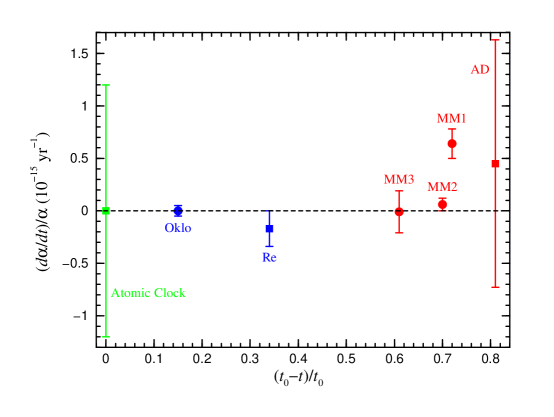
Figure 25: Constraints on the rate of variation $(d\alpha/dt)/\alpha$ as a function of the fractional “look-back” time $(t_{0}-t)/t_{0}$, where $t_{0}\approx 13$ Gyr is the present age of the Universe. The results shown are taken from data on atomic clocks [168], considerations of the Oklo phenomenon [160], meteoritic data on ¹⁸⁷Re decay [164, 166], and many-multiplet (MM1[151], MM2 [154], MM3 [155]) and alkali-doublet (AD [152]) analyses of quasar absorption spectra. For convenience, the results for MM1, MM2, MM3, and AD are shown at the mean redshift for the data used and then converted to $(t_{0}-t)/t_{0}$. Note that the result for MM1 actually covers $(t_{0}-t)/t_{0}=0.37$–0.84. Except for this result, all others are consistent with no time variation of $\alpha$.

The result found in [154] and in the statistically dominant subsample of 74 out of the 128 low redshift absorbers used in [151] are sensitive to the assumed isotopic abundance ratio of Mg. In both analyses, a solar ratio of ²⁴Mg:²⁵Mg:²⁶Mg = 79:10:11 was adopted. However, the resulting shift in $\alpha$ is very sensitive to this ratio. Furthermore, it is commonly assumed that the heavy Mg isotopes are absent in low metallicity environments characteristic of quasar absorption systems. Indeed, had the analyses assumed only pure ²⁴Mg is present in the quasar absorbers, a much more significant result would have been obtained. The Keck/Hires data[151] would have yielded $\Delta\alpha/\alpha=(-0.98\pm 0.13)\times 10^{-5}$ for the low redshift subsample and $\Delta\alpha/\alpha=(-0.36\pm 0.06)\times 10^{-5}$ for the VLT/UVES data[154].

The sensitivity to the Mg isotopic ratio has led to a new interpretation of the many multiplet results[171]. The apparent variation in $\alpha$ in the Fe-Mg systems can be explained by the early nucleosynthesis of ^25,26Mg. The heavy Mg isotopes are efficiently produced in intermediate mass stars, particular in stars with masses 4-6 times the mass of the sun, when He and H are burning in shells outside the C and O core. There may even be evidence for enhanced populations of intermediate mass stars at very low metallicity.

Recall the dispersion seen in D/H observations in quasar absorption systems as seen in Fig. 18. Is there a real dispersion in D/H in these high redshift systems? The data may show an inverse correlation of D/H abundance with Si [100, 102]. This may be an artifact of poorly determined Si abundances, or (as yet unknown) systematics affecting the D/H determination in high-column density (damped Lyman-$\alpha$, hereafter DLA) or low-column density (Lyman limit systems) absorbers. On the other hand, if the correlation is real it would indicate that chemical evolution processes have occurred in these systems and that some processing of D/H must have occurred even at high redshift.

It is interesting to speculate[172] that the possible high redshift destruction of D/H is real and related to the chemical evolutionary history of high red shift systems. For example, these observations could be signatures of an early population of intermediate-mass stars characterized by an initial mass function different from that of the solar neighborhood. An example of such an IMF is shown in Fig. 26 [173].

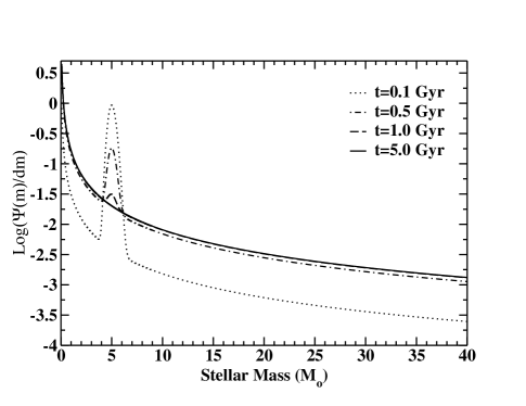
Figure 26: An IMF with an early enhancement of intermediate mass stars[173].

There are a number of immediate consequences of an IMF of the type shown in Fig. 26. In addition to the destruction of D/H at low metallicity, one expects observable C and N enhancements in high redshift absorption systems. In addition, one also expects an enhancement of the heavy Mg isotopes, ^25,26Mg, which may account[171, 173] for the apparent variation of the fine-structure constant in quasar absorption systems. In this sense, the many multiplet method can be used to trace the chemical history of primitive absorption clouds[171]. This hypothesis will be tested by future observations and examinations of correlation among other heavy elements produced in intermediate mass stars[174].

References

- [1] R. A. Alpher and R. C. Herman, Phys. Rev. 74, 1737 (1948); Phys. Rev. 75, 1089 (1949).
- [2] J. C. Mather, et al., Ap.J. 512 (1999) 511.
- [3] A. T. Lee et al., Ap. J. 561 (2001) L1 [arXiv:astro-ph/0104459]; R. Stompor et al., Ap.J. 561 (2001) L7 [arXiv:astro-ph/0105062].
- [4] C. B. Netterfield et al. [Boomerang Collaboration], Ap. J. 571 (2002) 604 [arXiv:astro-ph/0104460]; J. e. Ruhl et al., Astrophys. J. 599 (2003) 786 [arXiv:astro-ph/0212229].
- [5] N. W. Halverson et al. MNRAS 568 (2002) 38 [arXiv:astro-ph/0104489]; C. Pryke, N. W. Halverson, E. M. Leitch, J. Kovac, J. E. Carlstrom, W. L. Holzapfel and M. Dragovan, Ap. J. 568 (2002) 46 [arXiv:astro-ph/0104490].
- [6] S. Padin, et al. Ap.J. 549 (2001) L1; T.J. Pearson et al. Ap.J. 591 (2003) 556.
- [7] . A. Rubino-Martin et al., Mon. Not. Roy. Astron. Soc. 341 (2003) 1084 [arXiv:astro-ph/0205367].
- [8] A. Benoit et al. [the Archeops Collaboration], Astron. Astrophys. 399 (2003) L25 [arXiv:astro-ph/0210306].
- [9] C. L. Bennett et al., Astrophys. J. Suppl. 148 (2003) 1; D. N. Spergel et al., Astrophys. J. Suppl. 148 (2003) 175.
- [10] C. l. Kuo et al. [ACBAR collaboration], Astrophys. J. 600 (2004) 32 [arXiv:astro-ph/0212289].
- [11] D. Scott and G. F. Smoot, Phys. Lett. B 592 (2004) 1.
- [12] A. G. Riess et al., A. J. 116 (1998) 1009; S. Perlmutter et al., Ap. J. 517 (1999) 565; A. G. Riess et al., Ap. J. 560 (2001) 49.
- [13] S. M. Faber and J. J. Gallagher, Ann. Rev. Astron. Astrophys. 17 (1979) 135.
- [14] A. Bosma, Ap. J. 86 (1981) 1825; V. C. Rubin, W. K. Ford and N. Thonnard, Ap. J. 238 (1980) 471; V. C. Rubin, D. Burstein, W. K. Ford and N. Thonnard, Ap. J. 289 (1985) 81; T. S. Van Albada and R. Sancisi, Phil. Trans. R. Soc. Land. A320 (1986) 447.
- [15] M. Persic and P. Salucci, Ap. J. Supp. 99 (1995) 501; M. Persic, P. Salucci, and F. Stel, MNRAS 281 (1996) 27P.
- [16] R. P. Saglia et al., Ap. J. 403 (1993) 567; C. M. Carollo et al., Ap. J. 411 (1995) 25; A. Borriello, P. Salucci, and L. Danese, MNRAS 341 (2003) 1109; A. Dekel, F. Stoehr, G. A. Mamon, T. J. Cox and J. R. Primack, arXiv:astro-ph/0501622.
- [17] K. A. Olive, arXiv:astro-ph/0301505.
- [18] for reviews see: A. D. Linde, Particle Physics And Inflationary Cosmology Harwood (1990); K. A. Olive, Phys. Rep. 190 (1990) 307; D. H. Lyth and A. Riotto, Phys. Rept. 314 (1999) 1 [arXiv:hep-ph/9807278].
- [19] M. Persic and P. Salucci, MNRAS 258 (1992) 14p.
- [20] M. Fukugita, C. J. Hogan, and P. J. E. Peebles, Ap. J. 503 (1998) 518.
- [21] M. G. Haehnelt, P. Madau, R. Kudritzki, and F. Haardt, Ap. J. 549 (2001) L151; D. Reimers, Sp. Sci. Rev. 100 (2002) 89.
- [22] D. J. Hegyi and K. A. Olive, Phys. Lett. 126B (1983) 28; Ap. J. 303 (1986) 56.
- [23] D. N. Schramm and G. Steigman, Ap. J. 243 (1981) 1.
- [24] S. D. M. White, C. S. Frenk and M. Davis, Ap. J. 274 (1983) 61.
- [25] C. S. Frenk, S. D. M. White and M.Davis, Ap. J. 271 (1983) 417.
- [26] J. R. Bond, J. Centrella, A. S. Szalay and J. Wilson, in Formation and Evolution of Galaxies and Large Structures in the Universe, ed. J. Andouze and J. Tran Thanh Van, (Dordrecht-Reidel 1983) p. 87.
- [27] S. S. Gerstein and Ya. B. Zeldovich, JETP Lett. 4 (1966) 647; R. Cowsik and J. McClelland, Phys. Rev. Lett. 29 (1972) 669; A. S. Szalay and G. Marx, A. A. 49 (1976) 437.
- [28] K. Kainulainen and K. A. Olive, in Neutrino Mass, eds. G. Altarelli and K. Winter, (Springer, Berlin) p. 53 [arXiv:hep-ph/0206163].
- [29] R. A. Croft, W. Hu and R. Dave, Phys. Rev. Lett. 83 (1999) 1092 [arXiv:astro-ph/9903335].
- [30] X. M. Wang, M. Tegmark and M. Zaldarriaga, Phys. Rev. D65 (2002) 123001 [arXiv:astro-ph/0105091].
- [31] Ø. Elgaroy et al., Phys. Rev. Lett. 89 (2002) 061301 [arXiv:astro-ph/0204152].
- [32] A. Lewis and S. Bridle, Phys. Rev. D66 (2002) 103511 [arXiv:astro-ph/0205436].
- [33] P. Hut, Phys. Lett. B69 (1977) 85; B. W. Lee and S. Weinberg, Phys. Rev. Lett. 39 (1977) 165; M. I. Vysotsky, A. D. Dolgov and Y. B. Zeldovich, Pisma Zh. Eksp. Teor. Fiz. 26 (1977) 200.
- [34] E. W. Kolb and K. A. Olive, Phys. Rev. D33 (1986) 1202; E: 34 (1986) 2531; L. M. Krauss, Phys. Lett. 128B (1983) 37.
- [35] R. Watkins, M. Srednicki and K. A. Olive, Nucl. Phys. B310 (1988) 693.
- [36] K. Enqvist, K. Kainulainen and J. Maalampi, Nucl. Phys. B317 (1989) 647.
- [37] K. Enqvist and K. Kainulainen, Phys. Lett. B264 (1991) 367.
- [38] K. Griest and M. Kamionkowski, Phys. Rev. Lett. 64 (1990) 615.
- [39] P. Hut and K. A. Olive, Phys. Lett. B87 (1979) 144.
- [40] S. Eidelman et al. Phys. Lett. B 592 (2004) 1.
- [41] S. Ahlen, et al., Phys. Lett. B195 (1987) 603; D. D. Caldwell, et al., Phys. Rev. Lett. 61 (1988) 510; M. Beck et al., Phys. Lett. B336 (1994) 141.
- [42] R. D. Peccei and H. R. Quinn, Phys. Rev. Lett. 37 (1977) 1440; Phys. Rev. D16 (1977) 1791; S. Weinberg, Phys. Rev. Lett. 40 (1978) 223; F. Wilczek, Phys. Rev. Lett. 40 (1978) 279.
- [43] J. E. Kim, Phys. Rev. Lett. 43 (1979) 103; M. A. Shifman, A. I. Vainshtein, and V. I. Zakharov, Nucl. Phys. B166 (1980) 493; M. Dine, W. Fischler, and M. Srednicki, Phys. Lett. 104B (1981) 199.
- [44] J. Preskill, M. B. Wise, and F. Wilczek, Phys. Lett. 120B (1983) 127; L. F. Abbott and P. Sikivie, Phys. Lett. 120B (1983) 133; M. Dine and W. Fischler, Phys. Lett. 120B (1983) 137.
- [45] G. Raffelt, Phys. Rep. 198 (1990) 1.
- [46] D. Dearborn, D. N. Schramm, and G. Steigman, Phys. Rev. Lett. 56 (1986) 26.
- [47] J. Ellis and K. A. Olive, Phys. Lett. 193B (1987) 525; R. Mayle, J. Wilson, J. Ellis, K. A. Olive, D. N. Schramm, and G. Steigman, Phys. Lett. 203B (1988) 188; 219B (1989) 515; G. Raffelt and D. Seckel, Phys. Rev. Lett. 60 (1988) 1793; 67 (1991) 2605; A. Burrows, T. Ressel, and M. S. Turner, Phys. Rev. D42 (1990) 1020; W. Keil, H. T. Janka, D. N. Schramm, G. Sigl, M. S. Turner and J. R. Ellis, Phys. Rev. D56 (1997) 2419.
- [48] J. Ellis, J.S. Hagelin, D.V. Nanopoulos, K.A. Olive and M. Srednicki, Nucl. Phys. B238 (1984) 453; see also H. Goldberg, Phys. Rev. Lett. 50 (1983) 1419.
- [49] J. Rich, M. Spiro and J. Lloyd-Owen, Phys.Rep. 151 (1987) 239; P. F. Smith, Contemp. Phys. 29 (1998) 159; T. K. Hemmick et al., Phys. Rev. D41 (1990) 2074.
- [50] L. E. Ibanez, Phys. Lett. 137B (1984) 160; J. Hagelin, G. L. Kane, and S. Raby, Nucl., Phys. B241 (1984) 638; T. Falk, K. A. Olive, and M. Srednicki, Phys. Lett. B339 (1994) 248 [arXiv:hep-ph/9409270].
- [51] see e.g. K.A. Olive and M. Srednicki, Phys. Lett. 205B (1988) 553.
- [52] The LEP Collaborations, the LEP Electroweak Working Group, and the SLD Heavy Flavour and Electroweak Groups, CERN-EP-2000-016.
- [53] L. E. Ibáñez and G. G. Ross, Phys. Lett. B110 (1982) 215; L.E. Ibáñez, Phys. Lett. B118 (1982) 73; J. Ellis, D.V. Nanopoulos and K. Tamvakis, Phys. Lett. B121 (1983) 123; J. Ellis, J. Hagelin, D.V. Nanopoulos and K. Tamvakis, Phys. Lett. B125 (1983) 275; L. Alvarez-Gaumé, J. Polchinski, and M. Wise, Nucl. Phys. B221 (1983) 495.
- [54] G. Steigman, K. A. Olive, and D. N. Schramm, Phys. Rev. Lett. 43 (1979) 239; K. A. Olive, D. N. Schramm, and G. Steigman, Nucl. Phys. B180 (1981) 497.
- [55] K. Griest and D. Seckel, Phys. Rev. D43 (1991) 3191.
- [56] J. Ellis, T. Falk, and K.A. Olive, Phys. Lett. B444 (1998) 367 [arXiv:hep-ph/9810360]; J. Ellis, T. Falk, K.A. Olive, and M. Srednicki, Astr. Part. Phys. 13 (2000) 181 [Erratum-ibid. 15 (2001) 413] [arXiv:hep-ph/9905481].
-
[57]
Joint LEP 2 Supersymmetry Working Group,
Combined LEP Chargino Results, up to 208 GeV,
http://lepsusy.web.cern.ch/lepsusy/www/inos_moriond01/charginos_pub.html. -
[58]
Joint LEP 2 Supersymmetry Working Group, Combined LEP
Selectron/Smuon/Stau Results, 183-208 GeV,
http://lepsusy.web.cern.ch/lepsusy/www/sleptons_summer02/slep_2002.html. -
[59]
LEP Higgs Working Group for Higgs boson searches, OPAL Collaboration,
ALEPH Collaboration, DELPHI Collaboration and L3
Collaboration,
Phys. Lett. B 565 (2003) 61 [arXiv:hep-ex/0306033].
Searches for the neutral Higgs bosons of the MSSM: Preliminary
combined results using LEP data collected at energies up to 209 GeV,
LHWG-NOTE-2001-04, ALEPH-2001-057, DELPHI-2001-114, L3-NOTE-2700,
OPAL-TN-699, arXiv:hep-ex/0107030; LHWG Note/2002-01,
http://lephiggs.web.cern.ch/LEPHIGGS/papers/July2002_SM/index.html. - [60] S. Heinemeyer, W. Hollik and G. Weiglein, Comput. Phys. Commun. 124 (2000) 76 [arXiv:hep-ph/9812320]; S. Heinemeyer, W. Hollik and G. Weiglein, Eur. Phys. J. C 9 (1999) 343 [arXiv:hep-ph/9812472].
- [61] S. Chen et al. [CLEO Collaboration], Phys. Rev. Lett. 87 (2001) 251807 [arXiv:hep-ex/0108032]; BELLE Collaboration, BELLE-CONF-0135. See also K. Abe et al. [Belle Collaboration], Phys. Lett. B511 (2001) 151 [arXiv:hep-ex/0103042]; B. Aubert et al. [BaBar Collaboration], arXiv:hep-ex/0207076.
- [62] C. Degrassi, P. Gambino and G. F. Giudice, JHEP 0012 (2000) 009 [arXiv:hep-ph/0009337], as implemented by P. Gambino and G. Ganis.
- [63] M. Carena, D. Garcia, U. Nierste and C. E. Wagner, Phys. Lett. B499 (2001) 141 [arXiv:hep-ph/0010003]; P. Gambino and M. Misiak, Nucl. Phys. B611 (2001) 338; D. A. Demir and K. A. Olive, Phys. Rev. D65 (2002) 034007 [arXiv:hep-ph/0107329]; T. Hurth, arXiv:hep-ph/0106050; Rev. Mod. Phys. 75, 1159 (2003) [arXiv:hep-ph/0212304].
- [64] [The Muon g-2 Collaboration], Phys. Rev. Lett. 92 (2004) 161802, hep-ex/0401008.
- [65] M. Davier, S. Eidelman, A. Höcker and Z. Zhang, Eur. Phys. J. C 31 (2003) 503, hep-ph/0308213; see also K. Hagiwara, A. Martin, D. Nomura and T. Teubner, Phys. Rev. D 69 (2004) 093003, hep-ph/0312250; S. Ghozzi and F. Jegerlehner, Phys. Lett. B 583 (2004) 222, hep-ph/0310181; M. Knecht, hep-ph/0307239; K. Melnikov and A. Vainshtein, Phys. Rev. D70 (2004) 113006 [arXiv:hep-ph/0312226]. J. de Troconiz and F. Yndurain, hep-ph/0402285.
- [66] J. R. Ellis, K. A. Olive, Y. Santoso and V. C. Spanos, Phys. Lett. B565 (2003) 176 [arXiv:hep-ph/0303043].
- [67] H. Baer and C. Balazs, JCAP 0305 (2003) 006 [arXiv:hep-ph/0303114].
- [68] A. B. Lahanas and D. V. Nanopoulos, Phys. Lett. B568 (2003) 55 [arXiv:hep-ph/0303130]; U. Chattopadhyay, A. Corsetti and P. Nath, Phys. Rev. D68 (2003) 035005 [arXiv:hep-ph/0303201]; C. Munoz, Int. J. Mod. Phys. A19, 3093 (2004) [arXiv:hep-ph/0309346] R. Arnowitt, B. Dutta and B. Hu, arXiv:hep-ph/0310103.
- [69] M. Drees and M. M. Nojiri, Phys. Rev. D47 (1993) 376; H. Baer and M. Brhlik, Phys. Rev. D53 (1996) 59; and Phys. Rev. D57 (1998) 567; H. Baer, M. Brhlik, M. A. Diaz, J. Ferrandis, P. Mercadante, P. Quintana and X. Tata, Phys. Rev. D63 (2001) 015007; A. B. Lahanas, D. V. Nanopoulos and V. C. Spanos, Mod. Phys. Lett. A16 (2001) 1229.
- [70] J. R. Ellis, T. Falk, G. Ganis, K. A. Olive and M. Srednicki, Phys. Lett. B510 (2001) 236 [arXiv:hep-ph/0102098].
- [71] J. L. Feng, K. T. Matchev and T. Moroi, Phys. Rev. D 61 (2000) 075005 [arXiv:hep-ph/9909334].
- [72] A. Romanino and A. Strumia, Phys. Lett. B 487 (2000) 165, hep-ph/9912301.
- [73] J. R. Ellis and K. A. Olive, Phys. Lett. B514 (2001) 114 [arXiv:hep-ph/0105004].
- [74] J. R. Ellis, K. A. Olive, Y. Santoso and V. C. Spanos, Phys. Rev. D69 (2004) 095004 [arXiv:hep-ph/0310356].
- [75] J. Ellis, K. Olive and Y. Santoso, Phys. Lett. B539 (2002) 107 [arXiv:hep-ph/0204192].; J. R. Ellis, T. Falk, K. A. Olive and Y. Santoso, Nucl. Phys. B652 (2003) 259 [arXiv:hep-ph/0210205].
- [76] J. Polonyi, Budapest preprint KFKI-1977-93 (1977); R. Barbieri, S. Ferrara and C.A. Savoy, Phys. Lett. 119B (1982) 343.
- [77] J. R. Ellis, K. A. Olive, Y. Santoso and V. C. Spanos, Phys. Lett. B573 (2003) 162 [arXiv:hep-ph/0305212]; Phys. Rev. D70 (2004) 055005 [arXiv:hep-ph/0405110].
- [78] J. R. Ellis, A. Ferstl, K. A. Olive and Y. Santoso, Phys. Rev. D67, 123502 (2003) [arXiv:hep-ph/0302032].
- [79] D. Abrams et al. [CDMS Collaboration], Phys. Rev. D66 (2002) 122003 [arXiv:astro-ph/0203500].
- [80] A. Benoit et al., Phys. Lett. B545 (2002) 43 [arXiv:astro-ph/0206271].
- [81] D. S. Akerib et al. [CDMS Collaboration], Phys. Rev. Lett. 93, 211301 (2004) [arXiv:astro-ph/0405033].
- [82] DAMA Collaboration, R. Bernabei et al., Phys. Lett. B436 (1998) 379.
- [83] J. Ellis, K. A. Olive, Y. Santoso and V. C. Spanos, arXiv:hep-ph/0502001.
- [84] T. P. Walker, G. Steigman, D. N. Schramm, K. A. Olive and K. Kang, Ap.J. 376 (1991) 51; S. Sarkar, Rep. Prog. Phys. 59 (1996) 1493; K. A. Olive, G. Steigman, and T. P. Walker, Phys. Rep. 333 (2000) 389; B. D. Fields and S. Sarkar, Phys. Rev. D66 (2002) 010001.
- [85] L. M. Krauss and P. Romanelli, Ap.J. 358 (1990) 47; N. Hata, R. J. Scherrer, G. Steigman, D. Thomas, and T. P. Walker, Ap.J. 458 (1996) 637.
- [86] M. Smith, L. Kawano, and R. A. Malaney, Ap.J. Supp. 85 (1993) 219.
- [87] K. M. Nollett and S. Burles, Phys. Rev. D61, 123505 (2000) [arXiv:astro-ph/0001440].
- [88] R. H. Cyburt, B. D. Fields and K. A. Olive, New Astron. 6 (1996) 215 [arXiv:astro-ph/0102179].
- [89] A. Coc, E. Vangioni-Flam, M. Cass’e and M. Rabiet, Phys. Rev. D65 (2002) 043510 [arXiv:astro-ph/0111077].
- [90] C. Angulo et al., Nucl. Phys. A656 (1999) 3.
- [91] A. Coc, E. Vangioni-Flam, P. Descouvemont, A. Adahchour and C. Angulo, Ap. J. 600 (2004) 544 [arXiv:astro-ph/0309480].
- [92] R.H. Cyburt Phys. Rev. D70 (2004) 023505 [arXiv:astro-ph/0401091].
- [93] P. Descouvemont, A. Adahchour, C. Angulo, A. Coc and E. Vangioni-Flam, ADNDT 88 (2004) 203 [arXiv:astro-ph/0407101].
- [94] P. D. Serpico, S. Esposito, F. Iocco, G. Mangano, G. Miele and O. Pisanti, Int. J. Mod. Phys. A19 (2004) 4431 [arXiv:astro-ph/0307213].
- [95] R. H. Cyburt, B. D. Fields and K. A. Olive, Astropart. Phys. 17 (2002) 87 [arXiv:astro-ph/0105397].
- [96] R. I. Epstein, J.M. Lattimer, and D.N. Schramm, Nature 263 (1976) 198.
- [97] H. W. Moos et al., Astrophys. J. Suppl. 140 (2002) 3 [arXiv:astro-ph/0112519].
- [98] D.D. Clayton, Ap.J. 290 (1985) 428; B.D. Fields, Ap.J. 456 (1996) 678.
- [99] S. Burles and D. Tytler, Ap.J. 499, 699 (1998); Ap.J. 507, 732 (1998).
- [100] J. M. O’Meara, D. Tytler, D. Kirkman, N. Suzuki, J. X. Prochaska, D. Lubin and A. M. Wolfe, Ap.J. 552, 718 (2001) [arXiv:astro-ph/0011179].
- [101] D. Kirkman, D. Tytler, N. Suzuki, J. M. O’Meara and D. Lubin, Ap. J. Supp. 149 (2003) 1 [arXiv:astro-ph/0302006].
- [102] M. Pettini and D. V. Bowen, Ap.J. 560, 41 (2001) [arXiv:astro-ph/0104474].
- [103] D. Kirkman, D. Tytler, S. Burles, D. Lubin, J.M. O’Meara, Ap.J. 529, 655 (1999).
- [104] S. D’Odorico, M. Dessauges-Zavadsky, and P. Molaro, A.A. 368 (2001) L21
- [105] N.H. Crighton, J.K. Webb, A. Ortiz-Gill, and A. Fernandez-Soto, MNRAS 355 (2004) 1042.
- [106] Y.I. Izotov, T.X. Thuan, and V.A. Lipovetsky, Ap.J. 435, 647 (1994); Ap.J.S. 108, 1 (1997); Y.I. Izotov, and T.X. Thuan, Ap.J. 500, 188 (1998).
- [107] B.E.J. Pagel, E.A. Simonson, R.J. Terlevich and M. Edmunds, MNRAS 255, 325 (1992).
-
[108]
E. Skillman and R.C. Kennicutt, Ap.J. 411, 655 (1993);
E. Skillman, R.J. Terlevich, R.C. Kennicutt, D.R. Garnett, and E. Terlevich, Ap.J. 431,172 (1994). - [109] K. A. Olive and G. Steigman, Ap.J. Supp. 97 (1995) 49 [arXiv:astro-ph/9405022]; K. A. Olive, E. Skillman and G. Steigman, Ap.J. 483 (1997) 788 [arXiv:astro-ph/9611166]; B. D. Fields and K. A. Olive, Ap. J. 506 (1998) 177 [arXiv:astro-ph/9803297].
- [110] Y. I. Izotov and T. X. Thuan, Ap.J. 602 (2004) 200.
- [111] K. A. Olive and E. D. Skillman, New Astron. 6 (2001) 119.
- [112] K. A. Olive and E. D. Skillman, ApJ 617 (2004) 29 [arXiv:astro-ph/0405588].
- [113] M. Peimbert, A. Peimbert, and M.T. Ruiz, Ap.J. 541, 688 (2000); A. Peimbert, M. Peimbert, and V. Luridiana, Ap.J. 565, 668 (2002).
- [114] F. Spite, and M. Spite, A.A. 115, 357 (1982); P. Molaro, F. Primas, and P. Bonifacio, A.A. 295 , L47 (1995); P. Bonifacio and P. Molaro, MNRAS 285, 847 (1997).
- [115] S.G. Ryan, J.E. Norris, and T.C. Beers, Ap.J. 523, 654 (1999).
- [116] B.D.Fields and K.A. Olive, New Astronomy, 4, 255 (1999); E. Vangioni-Flam, M. Cassé, R. Cayrel, J. Audouze, M. Spite, and F. Spite, New Astronomy, 4, 245 (1999).
- [117] S.G. Ryan, T.C. Beers, K.A. Olive, B.D. Fields, and J.E. Norris, Ap.J. Lett. 530, L57 (2000).
- [118] B.D. Fields and K.A. Olive, Ap.J. 516, 797 (1999).
- [119] P. Bonifacio, et al., A.A. 390 (2002) 91.
- [120] L. Pasquini and P. Molaro, A.A. 307 (1996) 761.
- [121] F. Thevenin et al., A.A. 373 (2001) 905.
- [122] P. Bonifacio, A.A. 395 (2002) 515.
- [123] R. H. Cyburt, B. D. Fields, K. A. Olive and E. Skillman, arXiv:astro-ph/0408033.
- [124] C.P. Deliyannis, P. Demarque, and S.D. Kawaler, Ap. J. Supp. 73 (1990) 21.
- [125] S. Vauclair,and C. Charbonnel, Ap. J. 502 (1998) 372; M. H. Pinsonneault, T. P. Walker, G. Steigman and V. K. Narayanan, Ap. J. 527 (1998) 180 [arXiv:astro-ph/9803073]; M. H. Pinsonneault, G. Steigman, T. P. Walker, and V. K. Narayanan, Ap. J. 574 (2002) 398 [arXiv:astro-ph/0105439]; O. Richard, G. Michaud and J. Richer, A.A. 431 (2005) 1 [arXiv:astro-ph/0409672].
- [126] J. Melendez and I. Ramirez, Ap. J. 615 (2004) L33 [arXiv:astro-ph/0409383].
- [127] B. D. Fields, K. A. Olive and E. Vangioni-Flam, arXiv:astro-ph/0411728.
- [128] R. H. Cyburt, B. D. Fields and K. A. Olive, Phys. Rev. D69 (2004) 123519 [arXiv:astro-ph/0312629].
- [129] Bahcall, J.N., Pinsonneault, M.H., & Basu, S. Ap.J. 555 (2001) 990.
- [130] S. N. Ahmed et al. [SNO Collaboration], Phys. Rev. Lett. 92, 181301 (2004) [arXiv:nucl-ex/0309004].
- [131] D.S. Balser, T.M. Bania, R.T. Rood, and T.L. Wilson, Ap.J. 510 (1999) 759.
- [132] K. A. Olive, D. N. Schramm, S. T. Scully and J. W. Truran, Ap.J. 479 (1997) 752 [arXiv:astro-ph/9610039].
- [133] T. M. Bania, R. T. Rood and D. S. Balser, Nature 415 (2002) 54.
- [134] E. Vangioni-Flam, K. A. Olive, B. D. Fields and M. Casse, Ap.J. 585 (2003) 611 [arXiv:astro-ph/0207583].
- [135] S. Weinberg, Phys. Rev. Lett. 48 (1982) 1303.
- [136] J. Ellis, A.D. Linde and D.V. Nanopoulos, Phys. Lett. 118B (1982) 59.
-
[137]
D. Lindley,
Ap.J. 294 (1985) 1;
J. R. Ellis, D. V. Nanopoulos and S. Sarkar,
Nucl. Phys. B259 (1985) 175;
R. Juszkiewicz, J. Silk and A. Stebbins, Phys. Lett. 158B (1985) 463;
D. Lindley, Phys. Lett. B171 (1986) 235; M. Kawasaki and K. Sato, Phys. Lett. B189 (1987) 23. M. H. Reno and D. Seckel, Phys. Rev. D37 (1988) 3441; S. Dimopoulos, R. Esmailzadeh, L. J. Hall and G. D. Starkman, Nucl. Phys. B311 (1989) 699; J. Ellis et al., Nucl. Phys. B337 (1992) 399; M. Kawasaki and T. Moroi, Ap.J. 452 (1995) 506 [arXiv:astro-ph/9412055]; E. Holtmann, M. Kawasaki, K. Kohri and T. Moroi, Phys. Rev. D60 (1999) 023506 [arXiv:hep-ph/9805405]; M. Kawasaki, K. Kohri and T. Moroi, Phys. Rev. D63 (2001) 103502 [arXiv:hep-ph/0012279]; K. Kohri, Phys. Rev. D64 (2001) 043515 [arXiv:astro-ph/0103411]. - [138] R. H. Cyburt, J. R. Ellis, B. D. Fields and K. A. Olive, Phys. Rev. D67 (2003) 103521 [arXiv:astro-ph/0211258].
- [139] G. Sigl, K. Jedamzik, D. N. Schramm and V. S. Berezinsky, Phys. Rev. D 52 (1995) 6682 [arXiv:astro-ph/9503094]. M. Kawasaki, K. Kohri and T. Moroi, arXiv:astro-ph/0402490 and arXiv:astro-ph/0408426.
- [140] J. Ellis, K.A. Olive, and E. Vangioni, astro-ph/0503023.
- [141] M. Asplund et al., (2004) in preparation; D. L. Lambert, AIP Conf. Proc. 743 (2005) 206 [arXiv:astro-ph/0410418].
- [142] J. R. Ellis, J. E. Kim and D. V. Nanopoulos, Phys. Lett. 145B (1984) 181; M. Kawasaki and T. Moroi, Prog. Theor. Phys. 93 (1995) 879 [arXiv:hep-ph/9403364] J. R. Ellis, D. V. Nanopoulos, K. A. Olive and S. J. Rey, Astropart. Phys. 4 (1996) 371 [arXiv:hep-ph/9505438]; M. Bolz, A. Brandenburg and W. Buchmuller, Nucl. Phys. B606 (2001) 518 [arXiv:hep-ph/0012052].
- [143] J. L. Feng, S. f. Su and F. Takayama, Phys. Rev. D 70 (2004) 063514 [arXiv:hep-ph/0404198]; J. L. Feng, S. Su and F. Takayama, Phys. Rev. D 70 (2004) 075019 [arXiv:hep-ph/0404231].
- [144] J. R. Ellis, K. A. Olive, Y. Santoso and V. C. Spanos, Phys. Lett. B 588 (2004) 7 [arXiv:hep-ph/0312262].
- [145] K. Jedamzik, Phys. Rev. D 70 (2004) 063524 [arXiv:astro-ph/0402344]; K. Jedamzik, Phys. Rev. D 70 (2004) 083510 [arXiv:astro-ph/0405583].
- [146] J. L. Feng, A. Rajaraman and F. Takayama, Phys. Rev. D 68 (2003) 063504 [arXiv:hep-ph/0306024].
- [147] B. A. Campbell and K. A. Olive, Phys. Lett. B345, 429 (1995) [arXiv:hep-ph/9411272].
- [148] V.V. Dixit and M. Sher, Phys. Rev. D37 (1988) 1097.
- [149] P. Langacker, G. Segre and M. J. Strassler, Phys. Lett. B528, 121 (2002) [arXiv:hep-ph/0112233].
- [150] J. K. Webb, V. V. Flambaum, C. W. Churchill, M. J. Drinkwater and J. D. Barrow, Phys. Rev. Lett. 82 (1999) 884 [arXiv:astro-ph/9803165]; M. T. Murphy et al., Mon. Not. Roy. Astron. Soc. 327 (2001) 1208 [arXiv:astro-ph/0012419]. J. K. Webb et al., Phys. Rev. Lett. 87 (2001) 091301 [arXiv:astro-ph/0012539]; M. T. Murphy, J. K. Webb, V. V. Flambaum, C. W. Churchill and J. X. Prochaska, Mon. Not. Roy. Astron. Soc. 327 (2001) 1223 [arXiv:astro-ph/0012420].
- [151] M. T. Murphy, J. K. Webb and V. V. Flambaum, arXiv:astro-ph/0306483.
- [152] M. T. Murphy, J. K. Webb, V. V. Flambaum, J. X. Prochaska and A. M. Wolfe, Mon. Not. Roy. Astron. Soc. 327, 1237 (2001) [arXiv:astro-ph/0012421]; A. F. Martinez Fiorenzano, G. Vladilo and P. Bonifacio, arXiv:astro-ph/0312270.
- [153] J. N. Bahcall, C. L. Steinhardt and D. Schlegel, Ap.J. 600, 520 (2004) [arXiv:astro-ph/0301507].
- [154] H. Chand, R. Srianand, P. Petitjean and B. Aracil, A.A. 417, 853 (2004) [arXiv:astro-ph/0401094]; R. Srianand, H. Chand, P. Petitjean and B. Aracil, Phys. Rev. Lett. 92, 121302 (2004) [arXiv:astro-ph/0402177].
- [155] R. Quast, D. Reimers and S. A. Levshakov, A.A. 415 (2004) 7 [arXiv:astro-ph/0311280].
- [156] P. Sisterna and H. Vucetich, Phys. Rev. D41 (1990) 1034; J. P. Uzan, Rev. Mod. Phys. 75 (2003) 403 [arXiv:hep-ph/0205340].
- [157] E. W. Kolb, M. J. Perry and T. P. Walker, Phys. Rev. D33, 869 (1986); R. J. Scherrer and D. N. Spergel, Phys. Rev. D47, 4774 (1993); L. Bergstrom, S. Iguri and H. Rubinstein, Phys. Rev. D60, 045005 (1999) [arXiv:astro-ph/9902157]; K.M. Nollett and R.E. Lopez, Phys. Rev. D66 (2002) 063507 [arXiv:astro-ph/0204325].
- [158] K. Ichikawa and M. Kawasaki, Phys. Rev. D65 (2002) 123511 [arXiv:hep-ph/0203006].
- [159] G. Rocha, R. Trotta, C. J. A. Martins, A. Melchiorri, P. P. Avelino and P. T. P. Viana, New Astron. Rev. 47, 863 (2003) [arXiv:astro-ph/0309205].
- [160] A. I. Shlyakhter, Nature 264 (1976) 340; T. Damour and F. Dyson, Nucl. Phys. B480 (1996) 37; Y. Fujii et al., Nucl. Phys. B573 (2000) 377.
- [161] K. A. Olive, M. Pospelov, Y. Z. Qian, A. Coc, M. Casse and E. Vangioni-Flam, Phys. Rev. D66 (2002) 045022 [arXiv:hep-ph/0205269].
- [162] P.J. Peebles and R.H. Dicke, Phys. Rev., 128, 2006 (1962); F.J. Dyson, in Aspects of Quantum Theory edited by A. Salam and E.P. Wigner (Cambridge U. Press), p. 213 (1972).
- [163] G.W. Lugmair and S.J.G. Galer, Geochim. Cosmochimica Acta 56, (1992) 1673.
- [164] M. I. Smoliar et al., Science 271, 1099 (1996).
- [165] M. Linder et al., Geochim. Cosmochimica Acta 53, 1597 (1989).
- [166] K. A. Olive, M. Pospelov, Y. Z. Qian, G. Manhes, E. Vangioni-Flam, A. Coc, and M. Casse, Phys. Rev. D69 (2004) 027701
- [167] H. Marion et al., Phys. Rev. Lett. 90, 150801 (2003).
- [168] S. Bize et al., Phys. Rev. Lett. 90, 150802 (2003).
- [169] M. Fischer et al., physics/0311128 (2003); and physics/0312086.
- [170] K. A. Olive and Y. Z. Qian, Phys. Today 57, 40 (2004).
- [171] T. Ashenfelter, G. J. Mathews and K. A. Olive, Phys. Rev. Lett. 92 (2004) 041102 [arXiv:astro-ph/0309197].
- [172] B.D. Fields, K.A. Olive, J. Silk, M. Cassé, and E. Vangioni-Flam, Ap.J. 563, 653 (2001).
- [173] T. P. Ashenfelter, G. J. Mathews and K. A. Olive, Ap.J. 615 (2004) 82 [arXiv:astro-ph/0404257.
- [174] M. G. Kozlov, V. A. Korol, J. C. Berengut, V. A. Dzuba and V. V. Flambaum, Phys. Rev. A 70 (2004) 062108 [arXiv:astro-ph/0407579].