The Multipole Vectors of WMAP, and their frames and invariants

Abstract

We investigate the Statistical Isotropy and Gaussianity of the CMB fluctuations, using a set of multipole vector functions capable of separating these two issues. In general a multipole is broken into a frame and $2\ell-3$ ordered invariants. The multipole frame is found to be suitably sensitive to galactic cuts. We then apply our method to real WMAP datasets; a coadded masked map, the Internal Linear Combinations map, and Wiener filtered and cleaned maps. Taken as a whole, multipoles in the range $\ell=2-10$ or $\ell=2-20$ show consistency with statistical isotropy, as proved by the Kolmogorov test applied to the frame’s Euler angles. This result in not inconsistent with previous claims for a preferred direction in the sky for $\ell=2,...5$. The multipole invariants also show overall consistency with Gaussianity apart from a few anomalies of limited significance (98%), listed at the end of this paper.

1 Introduction

The recent WMAP data has enabled analysis of the CMB to much higher precision than ever before. The CMB acts like a curtain on the early universe and a back light on later times. It is also the largest thing we can observe, and therefore is a strong probe of features on cosmological scales. Inflationary theories predict the CMB fluctuations to be Gaussian and Statistically Isotropic (SI); the WMAP data should be the best way to test these predictions. Unfortunately, there have been reports of quite severe anomalies in this respect (Coles & al, 2003; Copi, Huterer, Starkman, 2003; Cruz & al, 2004; Donoghue, Donoghue, 2004; Eriksen & al, 2003, 2004a, 2004b; Hansen & al, 2004a; Hansen, Banday, Gorski, 2004; Ralston, Jain, 2004; Land, Magueijo, 2004a, 2005; Larson, Wandelt, 2004; Oliveira-Costa & al, 2003; Vielva & al, 2003; Park, 2003; Schwarz & al, 2003).

Specifically, significant hemisphere asymmetries have been detected(Eriksen & al, 2003; Hansen, Banday, Gorski, 2004; Land, Magueijo, 2004a), as have multipole alignments(Tegmark, Oliveira-Costa, Hamilton, 2003; Oliveira-Costa & al, 2003; Copi, Huterer, Starkman, 2003; Schwarz & al, 2003; Land, Magueijo, 2005), implying the onset of a preferred direction. Such statistical anisotropy would be in conflict with inflationary theories, in the sense that any inflation model which left the universe just large enough to observe any anisotropy induced by, for example, a non-trivial topology (Weeks & al, 2004; Tegmark, Oliveira-Costa, Hamilton, 2003; Roukema & al, 2004; Cornish & al, 2004), would require extreme fine tuning. This aside, it is interesting to consider possible origins of anisotropy in the universe: primordial magnetic fields, strings or walls (Berera & al, 2003), or an intrinsically inhomogeneous Universe (Moffat, 2005).

In this paper we build on the work of Tegmark, Oliveira-Costa, Hamilton (2003); Copi, Huterer, Starkman (2003); Land, Magueijo (2004b), re-examining the issue of multipole alignment in the light of a formalism based on the Maxwell multipole vectors. These are an elegant way of extracting the extra degrees of freedom beside the power spectrum contained in a given multipole. As explained in Land, Magueijo (2004b), it is important to convert these vectors into $2\ell-3$ invariants (a generalisation of the concept of eigenvalue) and an orthonormal triad of vectors (a generalisation of the concept of eigenvectors of a hermitian matrix). Such an operation neatly separates the issues of non-Gaussianity and of violations of statistical isotropy. We proposed such a scheme in Land, Magueijo (2004b), and a further study appeared in Dennis (2004b), with analytical distributions provided.

The plan of our paper is as follows. In Section 2 we distinguish SI and non-Gaussianity in real and harmonic (Fourier) space. Then in Section 3 we review previous work done with multipole vectors, their invariants and frames, and present our new proposal. In Section 4 we demonstrate the effectiveness of the method with simulations, and we apply these techniques to a variety of renditions of the WMAP data in Section 5. In the face of some concrete problems raised by real life data we conclude with an appraisal of our method, and how it stands in light of recent claims for anomalies in Section 6. This paper is to be seen as a technical companion paper to Land, Magueijo (2005) where the focus is more heavily placed on the analysis of the reported anomalies.

2 Statistical Isotropy and Gaussianity

First we outline the definitions and implications of Statistical Isotropy and Gaussianity in terms of the terminology of Real and Fourier space.

2.1 Real space

We consider the the temperature of the CMB photons received from different directions, $\hat{n}$, in terms of the fluctuation $\Delta T(\hat{n})=T(\hat{n})-\bar{T}$. Due to the random nature of the quantum fluctuations that seeded the initial perturbations (according to current standard cosmological models), our theories of this process can only determine the statistical behaviour of $\Delta T(\hat{n})$. A theory can only make definite predictions for ensemble averages: averages taken over an infinity of universes.

One way to characterise all the statistical information of the $\Delta T$ field is through the n-point correlation functions:

$$\langle\Delta T(\hat{n_{1}})\Delta T(\hat{n_{2}})...\Delta T(\hat{n_{n}})\rangle$$ (1)

Note that without SI, these functions depend on $\hat{n_{1}},\hat{n_{2}},...,\hat{n_{n}}$.

A function, f(r), is statistically isotropic if its statistical properties are invariant under translations ${\bf r}\rightarrow{\bf r}+\delta{\bf r}$, and there is no preferred direction (Hajian, Souradeep, 2005). On the surface of a sphere, this is equivalent to the statistical properties being rotationally invariant. Statistical Isotropy of the temperature fluctuations therefore demands that the n-point correlation functions are invariant under rotations. They now only depend on the magnitude of the separation between the vectors, $|\hat{n_{i}}-\hat{n_{j}}|$. For example, the 2-point function only depends on the distance between the 2 vectors, or equivalently the dot product:

$$\langle\Delta T(\hat{n_{1}})\Delta T(\hat{n_{2}})\rangle=C(\hat{n_{1}}.\hat{n_{2}})$$ (2)

As mentioned, our models of the early universe can make predictions for the statistical properties of the field $\Delta T(\hat{n})$. The simplest models of inflation predict the $\Delta T(\hat{n})$ to be a Gaussian random field. For a Gaussian field the n-point correlation functions are zero for odd n, and can be expressed in terms of the 2-point correlation function for even n. Therefore, the two-point correlation function contains all the statistical information for a Gaussian field.

The combination of SI and Gaussianity means the two point correlation function contains all the information AND it is rotationally invariant.

2.2 Fourier Space

The usual approach to analysing CMB data, is to expand the function $\Delta T(\hat{n})$ in terms of the spherical harmonics, and therefore work with the spherical harmonic coefficients; $a_{\ell m}$.

$$\Delta T(\hat{n})=\sum_{\ell,m}a_{\ell m}Y_{\ell m}(\hat{n})$$ (3)

We can translate properties of the function $\Delta T(\hat{n})$ into properties of the $a_{\ell m}$. As mentioned in Section 2.1, SI of $\Delta T(\hat{n})$ requires the 2-point correlation function of $\Delta T(\hat{n})$ to be rotationally invariant. The consequence for the $a_{\ell m}$ is that the 2-point correlation function be of the form (Hu, 2001):

$$\langle a_{\ell_{1}m_{1}}a_{\ell_{2}m_{2}}\rangle=C_{\ell_{1}}\delta_{{\ell_{1}}{\ell_{2}}}\delta_{{m_{1}}{m_{2}}}$$ (4)

We call $C_{\ell}$ the power spectrum.

Similarly, requiring the 3-point correlation function in real space to be SI demands that the 3-point function of the $a_{\ell m}$s be of the form (Hu, 2001):

$$\langle a_{\ell_{1}m_{1}}a_{\ell_{2}m_{2}}a_{\ell_{3}m_{3}}\rangle=\left(\begin{array}[]{ccc}\ell_{1}&\ell_{2}&\ell_{3}\\ m_{1}&m_{2}&m_{3}\end{array}\right)B_{\ell_{1}\ell_{2}\ell_{3}}$$ (5)

We call $B_{\ell_{1}\ell_{2}\ell_{3}}$ the Bi-spectrum.

Gaussianity of the temperature fluctuations $\Delta T(\hat{n})$ demands that the coefficients, $a_{\ell m}$, are gaussian random variables. Therefore, all the information about the field is contained in the 2-point correlation function $\langle a_{\ell_{1}m_{1}}a_{\ell_{2}m_{2}}\rangle$. All higher n-point correlations functions are to be obtained from the 2-point function by means of Wick’s theorem.

Therefore, in Fourier space terminology, the combination of SI and Gaussianity means the power spectrum $C_{\ell}$ contains all the information of the field.

3 Multipoles and the Multipole Vectors

A multipole, $T_{\ell}$, represents all the fluctuations in $\Delta T$ of a certain scale, $\ell\sim 1/\theta$. That is:

$$\Delta T(\hat{n}) = \sum_{\ell}{T_{\ell}(\hat{n})}$$ (6)

$$T_{\ell}(\hat{n}) = \sum_{m}{a_{\ell m}Y_{\ell m}(\hat{n})}$$ (7)

The reality of $\Delta T$ means $a_{\ell-m}$ is determined by $a_{\ell m}$ and Im$(a_{\ell 0})=0$. There are therefore $2\ell+1$ degrees of freedom in multipole $T_{\ell}$.

As discussed, SI demands that the n-point correlation functions be rotationally invariant, and in Fourier space this has consequences for the form the n-point functions $\langle a_{\ell_{1}m_{1}}....a_{\ell_{n}m_{n}}\rangle$ can take. In Equation 4 we can see that SI demands that the $a_{\ell m}$s depend only on $\ell$ (no m-preference) and are independent for different $\ell$ (no inter-$\ell$ correlations). If we think about it in terms of the p.d.f of each $a_{\ell m}$, the assumption of Gaussianity means that the shape of these p.d.f are Gaussian, and the assumption of SI means that their scaling are the same for the $a_{\ell m}$s of the same multipole, and independent for different multipoles. In fact, one can see that m-preference would indicate a preferred frame because the $a_{\ell m}$s are not frame independent, they depend on the frame of the Fourier Transform. Therefore, any m-preference would be related to a particular frame.

3.1 Separation of degrees of freedom for the quadrupole

A multipole is an irreducible representation of the SO(3) group. Therefore, from its $2\ell+1$ degrees of freedom we should be able to extract 3 rotational degrees of freedom, i.e., an orthonormal frame. SI requires no inter-$\ell$ correlations, and therefore the orthonormal frames of each multipole are independent. Equivalently, SI requires these frames to be uniformly distributed. The remaining $2\ell-2$ degrees of freedom (d.o.f) will be invariants. Of these, one can be the overall power in the multipole $C_{\ell}$ (a Gaussian d.o.f). The remaining $2\ell-3$ invariants would probe m-preference and the Gaussianity of that multipole (these invariants should be independent for different multipoles).

Therefore, if one separates the 3 rotational d.o.f from the invariants one can test SI in the form of no inter-$\ell$ correlations independently from the remaining issues of m-preference and Gaussianity.

For the example of the quadrupole there is a simple way of separating the d.o.f (Magueijo, 1994):

$$\delta T_{2}=Q_{ij}x^{i}x^{j}$$ (8)

where $Q_{ij}$ is a symmetric traceless matrix. From this matrix one may extract three eigenvectors and two independent combinations of invariant eigenvalues $\lambda_{i}$ (they sum to 0). The eigenvalues d.o.fs are essentially the power spectrum $C_{2}$ (related to the sum of the squares of $\lambda_{i}$) and the bispectrum $B_{2,2,2}$ (related to the determinant of the matrix, or the product of $\lambda_{i}$). The eigenvectors provide us with the orthonormal frame.

3.2 A general multipole

In Land, Magueijo (2004b) a new method was proposed that generalises this construction for any multipole. It built on the work of Copi, Huterer, Starkman (2003) who first introduced the Multipole Vector formalism in CMB analysis. They showed that a multipole can be represented in terms of $\ell$ unit vectors and an overall magnitude. The method has received much attention, from mathematicians securing and exploring features of the formalism (Dennis, 2004a, b; Katz, Weeks, 2004; Lachièze-Rey, 2004; Weeks, 2004), and from astrophysicists applying it to the WMAP data (Copi, Huterer, Starkman, 2003; Schwarz & al, 2003). In fact the formalism was first discovered by Maxwell (Maxwell, 1891). He showed that for a real function $f(x,y,z)$ which is an eigenfunction of the Laplacian on the unit sphere with eigenvalue $-\ell(\ell+1)$ (i.e., a spherical harmonic $Y_{\ell m}$), there exists $\ell$ unit vectors ${\bf v}_{1},...,{\bf v}_{\ell}$ such that:

$$f(x,y,z)=\nabla_{{\bf v}_{1}}...\nabla_{{\bf v}_{\ell}}\frac{1}{r}$$ (9)

where $\nabla_{{\bf v}_{1}}={\bf v}_{1}.\nabla$ is the directional derivative operator, and $r=\sqrt{x^{2}+y^{2}+z^{2}}$. A more useful form of the representation is given by (Dennis, 2004a):

$$f({\bf r})=A({\bf r}.{\bf v}_{1})...({\bf r}.{\bf v}_{\ell})+r^{2}R$$ (10)

where is $A$ is a constant, and R is a complicated term fully defined by the components of the ${\bf v}_{i}$.

With the Multipole Vector method, the $2\ell+1$ d.o.f are separated into $\ell$ unit vectors, $v_{i}$, and one invariant, A. In Land, Magueijo (2004b) we proposed a further step of selecting 2 of the vectors as “anchor vectors” (we discuss this step further in Section 3.3). You then use these anchor vectors ($L_{1},L_{2}$) to define an orthonormal frame:

$$x=\widehat{(L_{1}-L_{2})}$$ (11)

$$y=\widehat{(L_{1}+L_{2})}$$ (12)

$$z=\widehat{(L_{1}\times L_{2})}$$ (13)

and $2\ell-3$ invariants:

$$X_{12}=L_{1}.L_{2}$$ (14)

$$X_{1j}=L_{1}.L_{j}$$ (15)

$$X_{2j}=L_{2}.L_{j}$$ (16)

for $j\geq 3$. We also showed how the power spectrum and bispectrum can be written in terms of the $X_{ij}$ and A.

Note that the Multipole Vectors are “headless” vectors: they do not have a defined direction. This can be clearly seen in Equation 10 where any change in the sign of a vector can be absorbed into the scalar $A$. Therefore, we have to be careful in the definition of our orthonormal frame. We impose possible directions on the “anchor vectors” by insisting that their directions satisfy $X_{12}\equiv L_{1}.L_{2}>0$. Therefore, these vectors can still point in either direction but their directions are not independent, and there are only 2 possible combinations. The $z$-axis is now uniquely defined, and the $x$, and $y$-axes are up to a rotation by $\pi$ around the $z$-axis. We simply reduce the allowed range for the Euler angles of the axes.

We now have an orthonormal frame defined by our anchor vectors; we call this the Multipole Frame. The remaining vectors’ information is contained in their angles. The minimum number of dot products needed to contain all the information about the vector positions is the $2\ell-3$ invariants $X_{ij}$. So we see that information about m-preference and Gaussianity are contained in the angles between vectors, i.e. their relative spread.

Gaussianity and SI determine the probability distribution of these angles (see Dennis (2004b) for an analytical expression). Departures from the expected spread would indicate a departure from SI and/or Gaussianity. It is not possible to probe the issues of m-preference and non-Gaussianity separately, however in some extreme cases of m-preference the vectors form clear structures. For pure m-preference there is a frame where $(\ell-m)$ of the vectors will line along the z-axis of this frame, and the remaining m vectors will form a 2m regular polygon in the x-y plane. We refer to this as a “Handle and Disc” structure, with the aligning vectors making the “Handle”, and the planar vectors forming the “Disc”.

Note that this method involves all the information contained in the multipoles, as opposed to methods that explore just one statistic e.g., $B_{\ell\ell\ell}$. This obviously has many advantages as it allows for a much more thorough investigation.

Figure 1: The Euler angles found for the Multipole frames of 1000 simulations, for multipoles $\ell=2-20$. The solid line is for the whole sky, and the dashed line is with the Kp0 masked applied.

3.3 Anchors

We now explain further how to select the anchor vectors essential for our separation of SI and non-Gaussian issues. We need an internal way of selecting these, i.e., a method that does not depend on any outside coordinate frame. However, we want the process to be repeatable so selecting them at random (as we’ve done before) is not satisfactory. For instance we may want to compare results for different frequency channels, so that the algorithm must be unambiguous as well as invertible.

One such way would be to define the vectors as the two most aligned, or most orthogonal. This would select a pair, but would not provide them or the remaining vectors with an order. This is not a problem in defining the frame. However, with no ordering of the ${X_{1j},X_{2j}}$ we cannot assess the agreement of individual values with the simulations; we can only study them as a set. Ideally we want to use every piece of information, and therefore we look for a way to order the vectors.

We achieve this in the following way. From the set of $\ell$ unordered vectors $\{v_{i}\}$, for every vector we sum the square of its dot products with all other vectors:

$$K_{i}=\sum_{j}(X_{i,j})^{2}$$ (17)

where $X_{ij}=v_{i}.v_{j}$. Every vector now has a corresponding value of $K_{i}$, and we can order them. For example let $L_{1}$ be the vector with the maximum $K_{i}$ value, and $L_{2}$ equal the vector with the second highest $K_{i}$ value, etc… so $L_{\ell}$ is the vector with the lowest $K_{i}$ value. We can now calculate the $2\ell-3$ $X_{ij}$ values, and use the vectors $L_{1}$ and $L_{2}$ to define the frame.

4 A simple application

A sky cut (e.g., imposed by the Kp0 mask) induces Anisotropy onto the sky. To investigate the effectiveness of our method we look at how well this Anisotropy is detected. We simulate 1000 Gaussian skies with noise and beam, and we look at the orthonormal frames before and after we apply the Kp0 mask. We find the multipole frame $\{{\bf x},{\bf y},{\bf z}\}$, as defined above, for multipoles $\ell=2-20$, and record the corresponding Euler angles $(\phi,\theta,\psi)$ . As mentioned in Section 3.2, due to the Multipole Vectors having no defined direction, the definition of the orthonormal axes is defined up to $({\bf x},{\bf y})\rightarrow({\bf-x},{\bf-y})$. Therefore there is an equivalence between orthonormal axes $\{{\bf x},{\bf y},{\bf z}\}\sim\{-{\bf x},-{\bf y},{\bf z}\}$, which translates into an equivalence between Euler angles $(\phi,\theta,\psi)\sim(\phi+\pi,\theta,\psi)$. Thus the allowed ranges for the Euler angles of our Multipole Frames are $\phi\in[0,\pi],\theta\in[0,\pi],\psi\in[-\pi,\pi]$.

In Figure 1 we plot histograms of the distributions found for the Euler angles. We see that without any sky-cut the distributions are uniform as expected. However, we also clearly see how the sky-cut then does induce anisotropy. The $\phi$ and $cos(\theta)$ distributions become non-uniform: $\theta$ peaks around $\pi/2$ ($z$-axis in galactic plane), and $\phi$ also around $\pi/2$ ($x$-axis aligns with galactic poles). This is unlike other measures, such as the bispectrum, which doesn’t get largely effected by sky cuts.

In fact, one can predict this result. In terms of the Fourier expansion in spherical harmonics, the effect of the mask is to remove power from the $m\sim\pm\ell$ in galactic coordinates. Therefore we are equivalently inducing m-preference towards the lower $m$’s. As discussed in Section 3.2, pure $m$-preference leads to a particular “Handle and Disc” configuration for the vectors, with $\ell-m$ vectors in the handle and $m$ in the disc. Therefore, for this induced preference towards the lower $m$’s we would expect a handle and disc structure (if only a subtle one) with most of the vectors in the handle. Our method of selecting the anchor vectors will then favour those in this handle as they will maximise $K_{i}$ through their small inter-angles with other handle members. If the anchor vectors belong to the handle, then the $x$-axis will align with this handle and therefore point to the galactic poles, the $y$-axis will not be well defined, and the $z$-axis will be perpendicular to the handle and therefore lying in the galactic plane.

$\ell=2$

$\ell=3$

$\ell=4$

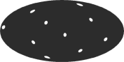
$\ell=5$

$\ell=6$

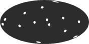
$\ell=7$

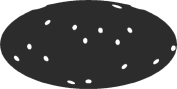
$\ell=8$

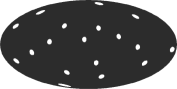
$\ell=9$

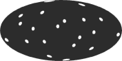
$\ell=10$

Figure 2: The Multipole Vectors for multipoles $\ell=2-10$ of the Kp0 masked Inverse-Noise-Squared coadded WMAP map, coadd. The vectors are headless, so each vector is represented by two white dots, where it intersects with the unit sphere.

$\ell=2$

$\ell=3$

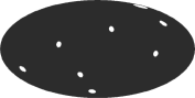
$\ell=4$

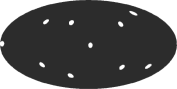
$\ell=5$

$\ell=6$

$\ell=7$

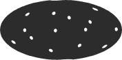
$\ell=8$

$\ell=9$

$\ell=10$

Figure 3: The Multipole Vectors for multipoles $\ell=2-10$ of the ILC WMAP map. The vectors are headless and each vector is represented by two white dots, where it intersects with the unit sphere.

5 Results

5.1 The datasets and methodology

We investigate the multipole vectors of the CMB using the WMAP data. We look at different representations of the data in the form of four different maps:

1. An Inverse-Noise-Squared Coadded map (coadd). We take the 8 foreground cleaned maps in the Q, V, and W bands, provided by WMAP. We combine these 8 data arrays ($DA_{i}$) using coefficients that maximally reduce the noise in the final map:

$$T(n)=\frac{\sum^{8}_{i=1}T_{i}(n)/\sigma^{2}_{i}}{\sum^{10}_{i=3}1/\sigma^{2}_{i}}$$ (18)

where $T_{i}(n)$ is the sky map for the DA $i$ with the foreground galactic signal subtracted, and

$$\sigma^{2}_{i} = {\sum^{Npix}_{n=1}1/\sigma^{2}_{i}(n)}$$ (19)

$$\sigma^{2}_{i}(n) = \sigma^{2}_{0,i}/Nobs_{i}(n)$$ (20)

$\sigma^{2}_{0,i}$ is the noise per observation for DA i, whose values are given by Bennett & al (2003). We apply the Kp0 mask to this map (Bennett & al, 2003) to cut possible remaining galactic contamination near the disk, and then we remove any residual monopole.

2. The Inter-Linear-Combination map (ILC), produced by the WMAP team (Bennett & al, 2003). This map is formed from a combination of smoothed maps, with weights chosen to maintain CMB anisotropy signal while minimizing the Galactic foreground. The WMAP team advise that the ILC map be used as a visual tool, and not used for CMB studies. We include it here for interest, as other groups have claimed interesting detections of anomalies in this map(Copi, Huterer, Starkman, 2003).

3+4. Tegmark, Oliveira-Costa, Hamilton (2003) produced their own foreground cleaned maps . Their approach did not assume a specific power spectrum, and these maps contain less foreground signals and noise than the ILC map. For the lowest multipoles the maps are clean enough that no galactic cut is required (Tegmark, Oliveira-Costa, Hamilton, 2003). Our third map is their cleaned map (TOHcl), and our fourth map is their Wiener filtered map (TOHw).

We will compare findings to those from simulations. Our simulations are of Gaussian fluctuations, with the noise and beam properties of the coadd map. We perform 1000 of these simulations with the Kp0 mask, and 1000 without. In the case of the coadd map we always compare the results to those with the Kp0 mask added, and for the other ILC, TOHcl, and TOHw maps we compare their results to those without the mask. We have only done simulations with the noise and beam properties of the coadd map to simplify matters. We find this acceptable as at the low-$\ell$ multipoles we are concentrating on, the difference in the levels of noise and resolution seen in the four maps are insignificant.

Throughout our analysis we use software produced by the HEALPix collaboration , Górski, Hivon, Wandelt (1999). To compute the Multipole Vectors we use codes produced by Copi, Huterer, Starkman (2003).

5.2 The Multipole vectors

In Figures 2,3 we display in Mollweide projection the multipole vectors for map coadd and ILC, for multipoles $\ell=2-10$ (for these multipoles the vectors for maps TOHcl and TOHw by eye look very similar to the ILC map results). Recall that these vectors are headless, so we show dots at both ends. In Figure 3 one can see the planarity of the $\ell=3$ multipole vectors, and the alignment of this plane with the galactic plane and the plane of the $\ell=2$ multipole vectors, as reported by Oliveira-Costa & al (2003); Copi, Huterer, Starkman (2003); Schwarz & al (2003); Weeks (2004). However, a word of warning, this visual projection can be misleading as other significant features would not be so apparent by eye. In this projection our eye easily picks out any planarity in the galactic plane.

We now use our prescription of defining “anchor vectors” to investigate the multipole-frames and the multipole-dots for each map. Therefore the analysis of CMB data now splits into two areas:

1. The Multipole Frames. We search for inter-$\ell$ correlations by looking for correlations between these frames. SI demands that the frames be uniformly orientated (apart from the effect of sky cuts, noise, etc). Any correlation between frames of different multipoles, apart from that seen in the simulations, would indicate statistical anisotropy. The simplest case would be an alignment of the frames - clearly indicating one preferred frame. We investigate this issue for our four maps in Section 5.3.

2. The Multipole Invariants. For each multipole we extract the $2\ell-3$ invariants, $X_{ij}$. From simulations we can extract their expected distributions assuming SI and Gaussianity taking into account additional factors such as noise and beam. We investigate this in Section 5.4.

5.3 The Multipole Frames

For each of the four maps we do the following. For each multipole in the range $\ell=2-20$ we find the Multipole Vectors, and order them as described in Section 3.3. We define $L_{1}$ and $L_{2}$ as the anchor vectors, and use these anchor vectors to define an orthonormal frame as described in Section 3.2.

Figure 4: The cumulative frequency plot of the Euler angles from the multipole frames of the Coadded WMAP map, for $\ell=2-20$. Dashed line= the corresponding expected distribution returned from simulations.

Under the hypothesis of Statistical Isotropy we expect these multipole frames to be uniformly distributed (except for the anisotropy induced by the galactic cut in the case of the coadd map). One cannot assess how uniformly distributed a frame is one at a time as clearly every orientation is just as likely and so no significance can be assigned to any particular result. One can only ask how probable it is that a number of frames came from a uniform distribution. To do this we use a Kolmogorov-Smirnov test. This provides a goodness of fit test for a statistical distribution. It looks at the discrepancy between the cumulative frequency of observations and the expected cumulative frequency. The maximum discrepancy is called the D-statistic. For large enough sample sizes there is an analytical expression for the critical values of the D-statistic, over which a null hypothesis should be rejected.

We calculate the cumulative frequency over a range of multipoles of the Euler angle observations, $\phi,cos(\theta),\psi$. We do this for two multipole ranges, $\ell=2-10$ and $\ell=2-20$. We compare the distributions we find for the maps to those from simulations. As expected, the distributions the simulations return are near uniform. For example, in Figure 4 we visualise the cumulative frequencies of the coadd map results, accumulated over multipoles $\ell=2-20$. The expected distribution returned by the simulations is also shown. The D-statistic is the maximum discrepancy between the two lines.

	$\phi$	$cos(\theta)$	$\psi$
		$\ell=2-10$
coadd	0.335(9.0)	0.205(51.5)	0.360(12.0)
ILC	0.079(92.3)	0.256(35.5)	0.284(26.2)
TOHcl	0.370(5.1)	0.174(73.8)	0.138(90.3)
TOHw	0.259(25.2)	0.145(87.7)	0.249(40.5)
		$\ell=2-20$
coadd	0.213(7.8)	0.187(25.3)	0.219(17.4)
ILC	0.130(49.0)	0.070(98.4)	0.069(95.9)
TOHcl	0.133(44.5)	0.225(14.8)	0.109(80.6)
TOHw	0.133(44.5)	0.075(94.1)	0.136(57.1)

Table 1: D-statistics from cumulative frequency distributions of the Multipole Frame Euler angles from multipoles $\ell=2-10$ and $\ell=2-20$.

For each of the four maps, and for both the $\ell$ ranges we find the maximum discrepancy, the D-statistic, that the 3 Euler angles find. As our sample sizes are relatively small (9 observations for $\ell=2-10$ range, and 19 for $\ell=2-20$) we do not use analytical expressions for the critical values of the D-statistic: we assess the significance of the D-statistics we observe by comparing them to all those the simulations found. In Table 1 we list the D-statistics found and, in brackets, the percentage of simulations that found larger values. A significant departure from the null hypothesis would result in a high D-statistic, and therefore a low percentage value. We find no significant evidence for any departure from the expected uniform (nearly uniform in the case of the coadd map) distribution for the multipole frames. Therefore, using our Multipole Frames we find no evidence for a departure from SI for multipoles $\ell=2-20$.

5.4 The Multipole Invariants

We now turn our attention to the invariant degrees of freedom. As discussed in Section 3.1, the invariants of one multipole will probe Gaussianity, and the m-preference associated with SI. In terms of the Multipole Vectors this information is stored in their relative spacing - the angles between one and another. Dennis (2004b) computed the analytical expression for the expectation of the general dot product for a given multipole.

For each multipole we will not look at all the dot products between all the vectors as this contains redundant information. We will use our prescription of defining anchor vectors, and observe the $2\ell-3$ invariants $X_{ij}$, as described in Section 3.1.

For each map, and for each multipole $\ell=2-20$ we calculate the $2\ell-3$ invariants $X_{ij}$. We compare their values to those from simulations. In Figure 5 we display the results found for the invariants $X_{12}$, $X_{13}$, and $X_{23}$. We also show the $\bar{X}_{ij}\pm\sigma$ values that the simulations returned.

Figure 5: The $X_{12}$, $X_{13}$, and $X_{23}$ results for the coadd map (bold line), the ILC map (short-dash), the TOHcl map (long-dash), and the TOHw map (dash-dot). Also shown is the mean, $\pm 1\sigma$ for the simulations (dotted), with and without the Kp0 mask added.

In these plots we can observe potentially anomalous features. For example in the $X_{12}$ plot the $\ell=5$ value is very low for the ILC, TOHcl, and TOHw maps, and the $\ell=13$ value is low for the coadd map. The $X_{13}$ plot again shows out-lier values for $\ell-5$ in the ILC map, and $\ell=13$ for the coadd map.

To assess the significance of the outliers, we compare the values of all the invariants $X_{ij}$ for multipoles $\ell=2-20$ to those from simulations: for each value we find the number of simulations that find a lower value. We highlight as anomalous any result where either $>$99% or $<$1% of the simulations found lower values, and we record just these results in Table 2.

$\ell$	i	j	%
coadd
11	1	5	0.8
12	1	6	1.0
13	1	3	0.8
13	2	8	0.6
13	1	9	99.1
14	2	14	99.7
15	2	12	0.4
16	1	11	99.5
ILC
6	1	2	0.9
11	1	9	99.6
13	1	6	99.7
13	2	10	99.5
16	2	10	99.0
18	1	4	99.5
18	1	6	0.2
18	2	8	99.4
19	1	5	99.5
TOHcl
3	2	3	0.8
8	2	4	99.5
13	1	6	0.4
14	1	9	0.6
16	2	13	99.0
19	2	10	99.4
TOHw
3	2	3	0.8
8	2	5	99.1
9	1	6	0.1
13	1	5	0.2
17	1	14	0.5
18	1	11	1.0
19	2	9	99.8
19	1	18	99.0
20	1	10	1.0

Table 2: Anomalous multipole invariant values, at the 98% significance level. The percentage of simulations that find lower values.

Before we take any of these results too seriously, we must note that a certain of number of anomalous values are expected. That is the same with any statistic. For each multipole there are $2\ell-3$ invariants that we measure. Therefore, when we look at the multipoles $\ell=2-20$ for each map we observe a total of 361 invariants. We have highlighted the values outside the 98% confidence interval, and so we would expect 2% of our observations to be highlighted: $\sim$7 results for every map. We see in the tables that the coadd map finds 8 “anomalies”, the ILC finds 9,TOHcl finds 6, and TOHw finds 9. We also expect to find these $\sim$7 values in the higher multipoles, as these return more invariants.

Bearing this in mind, we highlight as particularly interesting the “anomalies” found in the low multipole $\ell=3$, for maps TOHcl and TOHw. This result shows a particularly low dot product between the second and third vectors, and therefore an unusually large angle.

Also of significance are the multipoles where 3 “anomalous” values are found: $\ell=13$ for the coadd map, and $\ell=18$ for the ILC map.

However, we conclude that through analysis of the Multipole Vectors there is no evidence for inherent non-Gaussianity or m-preference in the multipoles $\ell=2-20$.

6 Discussion

With improving CMB observations, the job of analysing the data also requires improved methods. It is unsatisfactory to investigate numerous statistics that bear no intuitive investigative properties. In particular, the issues of SI and Gaussianity should be probed separately.

In this paper we have applied a method proposed in Land, Magueijo (2004b) to the WMAP data. The method uses all the information in a map, and separates out the issues of SI and Gaussianity by defining an orthonormal frame (Multipole Frame) for each multipole, and a set of invariants (Multipole Invariants). In theory, the robustness of this method makes it ideal for a thorough investigation of anomalies in the CMB.

We analysed the Multipole Vectors of four different CMB maps, all derived from the WMAP data. We looked at the multipoles $\ell=2-20$, and for each multipole we found a Multipole Frame and the Multipole Invariants. To investigate the Statistical Isotropy of the data we analysed the orientation of the Multipole Frames over 2 separate multipole ranges, $\ell=2-10$, and $\ell=2-20$. We found no evidence that the Euler angles of these frames significantly favoured any particular values. Therefore we found no evidence for a departure from SI. To investigate the Non-Gaussianity of the data we analysed all the 361 Multipole Invariants for multipoles $\ell=2-20$ and compared their values to those from simulations. We recorded the extreme values, and saw that each map found approximately the expected amount. Therefore we found no evidence for Non-Gaussianity.

In light of previously detected anomalies (Coles & al, 2003; Copi, Huterer, Starkman, 2003; Land, Magueijo, 2005; Oliveira-Costa & al, 2003; Ralston, Jain, 2004; Schwarz & al, 2003; Tegmark, Oliveira-Costa, Hamilton, 2003), the failure of our method to return any significant results raises a couple of interesting points. The effectiveness of our method comes into question, and in practice we have seen that our method is victim to discontinuous noise. The method pivots around the selection of Anchor Vectors. Small fluctuations in the positions of the Multipole Vectors alters their ordering and therefore has a large effect on our method. The Anchor vectors can then differ, and this induces a discontinuous noise in the Euler angles of the Multipole Frames and in the Multipole Invariants. Also, different ways of ordering the vectors will make the method effective at detecting different features.

Another significant issue raised is that of priors. In this paper we limit ourselves to the multipoles $\ell=2-20$, but we do not focus any further or assume priors about any range. Therefore we may overlook interesting features in a few multipoles because their anomalous behaviour will be diluted by the well behaved values from other multipoles. In only focusing on interesting multipoles one has assumed a prior. In this paper we have applied our method to look for more overall features.

We conclude that the Multipole Vector method with the anchor vectors is technically ideal, but in practice is very limited by noise. In its application we have found no evidence for anisotropy or non-gaussianity. However, we feel that in light of other reported results this is because our method overlooks subtle features in the data. What we gain in thoroughness, we loose in sensitivity. We find no evidence for inherent anisotropy or Non-Gaussianity.

References

- Bennett & al (2003) Bennett C., et al., 2003, Astrophys J Suppl. 148 1.
- Bennett & al (2003) Bennett C., et al., 2003, Astrophys J Suppl. 148 97.
- Berera & al (2003) Berera A., Buniy R., Kephart T., hep-th/0311223.
- Coles & al (2003) Coles P., et al., 2003, astro-ph/0310252
- Copi, Huterer, Starkman (2003) Copi C.J., Huterer D., Starkman G.D., 2003, astro-ph/0310511
- Cornish & al (2004) Cornish N., et al., Phys. Rev. Lett. 92, 201302, 2004.
- Cruz & al (2004) Cruz M., et al., 2004, astro-ph/0405341
- Dennis (2004a) Dennis M.R., 2004a, math-ph/0408046
- Dennis (2004b) Dennis M.R., 2004b, math-ph/0410004
- Donoghue, Donoghue (2004) Donoghue E.P., Donoghue J.F., 2004, astro-ph/0411237
- Eriksen & al (2003) Eriksen H.K., et al, 2y003, astro-ph/0307507
- Eriksen & al (2004a) Eriksen H.K., et al, 2004a, astro-ph/0401276
- Eriksen & al (2004b) Eriksen H.K., et al, 2004b, astro-ph/0407271
- Hajian, Souradeep (2005) Hajian A., Souradeep T., 2005, astro-ph/0501001
- Górski, Hivon, Wandelt (1999) Górski K.M., Hivon E., Wandelt B., 1999, astro-ph/9905275
- Hansen & al (2004a) Hansen F.K. et al., 2004a, astro-ph/0402396
- Hansen, Banday, Gorski (2004) Hansen F.K., Banday A.J., Gorski K.M., 2004, astro-ph/0404206
- Hu (2001) Hu W., 2001, astro-ph/0105117
- Katz, Weeks (2004) Katz G., Weeks J., 2004, astro-ph/0405631
- Lachièze-Rey (2004) Lachièze-Rey M., 2004, astro-ph/0409081
- Land, Magueijo (2004a) Land K.R., Magueijo J., 2004a, astro-ph/0405519
- Land, Magueijo (2004b) Land K.R., Magueijo J., 2004b, astro-ph/0407081
- Land, Magueijo (2005) Land K.R., Magueijo J., 2005, astro-ph/0502237
- Larson, Wandelt (2004) Larson D.L., Wandelt B.D., 2004, astro-ph/0404037
- Magueijo (1994) Magueijo J.C.R., 1994, astro-ph/9412096
- Maxwell (1891) Maxwell J.C., 1891, A Treatise on Electricity and Magnetism, Clarendon Press
- Moffat (2005) Moffat J., astro-ph/0502110.
- Oliveira-Costa & al (2003) Oliveira-Costa A. et al., 2003, astro-ph/0307282
- Park (2003) Park C., 2003, astro-ph/0307469
- Ralston, Jain (2004) Ralston J.P., Jain P., 2004, astro-ph/0311430
- Roukema & al (2004) Roukema B.F., et al., astro-ph/0402608.
- Schwarz & al (2003) Schwarz D.J. et al., 2003, astro-ph/0403353
- Tegmark, Oliveira-Costa, Hamilton (2003) Tegmark M., Oliveira-Costa A., Hamilton J.S., 2003, Phys.Rev.D68(2003)123523
- Vielva & al (2003) Vielva P., et al., 2003, astro-ph/0310273
- Weeks (2004) Weeks J., 2004, astro-ph/0412231
- Weeks & al (2004) Weeks J., et al., Mon. Not. Roy. Astron. Soc. 352, 258, 2004.