A test for the universality of extinction curve shape

Abstract

We present an analysis of 436 lines of sight with extinction data covering wavelength range from near-infrared (NIR) to ultraviolet (UV). We use $J,H,K$ photometry from 2MASS database, the IR intrinsic colors from Wegner (1994), and UV extinction data from Wegner (2002). We exclude 19 lines of sight (4%) from the original sample because of suspected photometric problems. We derive total to selective extinction ratios ($R_{V}$) based on the Cardelli, Clayton, & Mathis (1989; CCM) law, which is typically used to fit the extinction data for both diffuse and dense interstellar medium. We conclude that CCM law is able to fit well most of the extinction curves in our sample (71%), and we present a catalog of $R_{V}$ and visual extinction ($A_{V}$) values for those cases. We divide the remaining lines of sight with peculiar extinction into two groups according to two main behaviors: a) the NIR or/and UV wavelength regions cannot be reproduced by CCM formula (14% of the entire sample), b) the NIR and UV extinction data taken separately are best fit by CCM laws with significantly different values of $R_{V}$ (10% of the entire sample). We present examples of such curves. We caution that some peculiarities of the extinction curves may not be intrinsic but simply caused by faulty data. The study of the intrinsically peculiar cases could help us to learn about the physical processes that affect dust in the interstellar medium, e.g., formation of mantles on the surface of grains, evaporation, growing or shattering.

Key words: catalogs — dust, extinction — Galaxy: general — ISM: structure — techniques: photometric

1 Introduction

The interstellar grains affect starlight which passes through them by absorbing and scattering photons. These two physical processes produce interstellar extinction which depends on the properties of dust grains, e.g., size distribution and composition. The extinction curve shows the extinction as a function of wavelength from the infrared to ultraviolet. Savage & Mathis (1979) presented the average extinction curve of our Galaxy at various wavelengths. It shows some evident features: it rises in the infrared, it shows a slight knee in the optical, it is characterized by a bump at 2175$\AA$, and it rises in the far-ultraviolet. These features are common between different environments. The interstellar grain properties are different in diffuse and dense interstellar medium and thus also the extinction changes. Cardelli, Clayton and Mathis (1989; hereafter CCM) found an average extinction law valid over the wavelength range $0.125\mu m\leq\lambda\leq 3.5\mu m$, which is applicable to both diffuse and dense regions of the interstellar medium. This extinction law depends on only one parameter, $R_{V}=A_{V}/E(B-V)$, where $A_{V}$ is the visual extinction and $E(B-V)$ is the color excess or reddening. The $R_{V}$ parameter ranges from about 2.0 to about 5.5 (with a typical value of 3.1) when one goes from diffuse to dense interstellar medium and thus $R_{V}$ characterizes the region that produces the extinction.

If one knows the value of $R_{V}$ along a particular line of sight, one can obtain the extinction curve at any wavelength $\lambda$ from the infrared to ultraviolet using CCM law:

$$\frac{A_{\lambda}}{A_{V}}=a(x)+b(x)\cdot R_{V}^{-1},$$ (1)

where $x=1/\lambda$, and $a(x)$ and $b(x)$ are the wavelength-dependent coefficients.

There are different ways to obtain $R_{V}$ using optical/NIR or UV extinction data. Wegner (2003) computed $R_{V}$ values for the sample of 597 OB stars for which the optical/NIR magnitudes are known. He assumed that, in the infrared spectral region, the normalized extinction curve is proportional to $\lambda^{-3}$ or $\lambda^{-4}$. Extrapolating the IR interstellar extinction curve to $1/\lambda=0$ he derived $R_{V}$ as:

$$R_{V}=-\left[\frac{E(\lambda-V)}{E(B-V)}\right]_{\lambda\longrightarrow\infty}.$$ (2)

Gnaciński & Sikorski (1999) applied the $\chi^{2}$ minimization method to compute $R_{V}$ values for a sample of ultraviolet (UV) extinction data using the linear relation (1). Geminale & Popowski (2004) extended the analysis of Gnaciński & Sikorski (1999) by using non-equal weights derived from observational errors to determine $R_{V}$ and $A_{V}$ values toward the sample of 782 stars with known ultraviolet color excesses.

In this paper we use both near-infrared ($JHK$) and UV photometry to obtain $R_{V}$ values for a sample of 436 lines of sight. We arrive at two main conclusions: (i) there are lines of sight with extinction in the NIR or/and UV which generically don’t follow CCM law, and (ii) there are lines of sight which show an extinction curve that cannot be reproduced with a single $R_{V}$ value in the whole wavelength range.

The structure of this paper is the following. In §2 we discuss the theoretical basis of the $\chi^{2}$ minimization method we use to derive $R_{V}$ values. In §3 we describe our data sources. In §4 we present the results and show two main peculiar classes of extinction curves present in our sample. Finally in §5 we summarize our results.

2 Theoretical Considerations

We normalize extinction in a standard way:

$$\epsilon(\lambda-V)=\frac{E(\lambda-V)}{E(B-V)}.$$ (3)

The absolute extinction may be deduced from the relative extinction by using total-to-selective extinction ratio $R_{V}$:

$$R_{V}=\frac{A_{V}}{E(B-V)},$$ (4)

because:

$$\epsilon(\lambda-V)=\frac{E(\lambda-V)}{E(B-V)}=\frac{A_{\lambda}-A_{V}}{E(B-V)}=R_{V}\left\{\frac{A_{\lambda}}{A_{V}}-1\right\}.$$ (5)

For each individual band, equation (1) and (5) can be combined to derive an $R_{V}$ value. More generally, the $\chi^{2}$ minimization can be used to obtain the $R_{V}$ value that provides the best CCM fit to all observed extinction data. Here we follow our previous method (Geminale & Popowski, 2004) and use a weighted formula to find $R_{V}$ by minimizing the following $\chi^{2}$:

$$\chi^{2}=\sum_{i=1}^{N_{\rm bands}}w_{\lambda_{i}}\{\epsilon(\lambda_{i}-V)-[R_{V}(a(x_{i})-1)+b(x_{i})]\}^{2}~{}E^{2}(B-V),$$ (6)

where $\omega_{i}\equiv 1/\sigma_{i}^{2}$ are the weights associated with each band, and $a(x_{i})$ and $b(x_{i})$ are the coefficients of CCM law.

Minimizing equation (6) with respect to $R_{V}$, yields:

$$R_{V}=\frac{\sum_{i=1}^{N_{\rm bands}}\{(a(x_{i})-1)\cdot(\epsilon(\lambda_{i}-V)-b(x_{i}))/\sigma_{i}^{2}\}}{\sum_{i=1}^{N_{\rm bands}}\{(a(x_{i})-1)^{2}/\sigma_{i}^{2}\}},$$ (7)

where in the current work $\sigma_{i}$ values are taken from Wegner (2002) and they were computed according to:

$$\sigma_{i}^{2}\equiv\sigma^{2}[\epsilon(\lambda_{i}-V)]=\left[\frac{1}{E(B-V)}\right]^{2}\,\left\{\sigma^{2}[E(B-V)]+[E(\lambda_{i}-V)]^{2}\,\sigma^{2}[E(\lambda_{i}-V)]\right\}$$ (8)

We compute the error in $R_{V}$ as:

$$\sigma(R_{V})\equiv\sum_{j=1}^{N_{\rm bands}}\left|\frac{\partial R_{V}}{\partial\epsilon(\lambda_{j}-V)}\right|\cdot\sigma_{j}=\frac{1}{\sum_{i=1}^{N_{\rm bands}}(a(x_{i})-1)^{2}/\sigma_{i}^{2}}\cdot\sum_{j=1}^{N_{\rm bands}}\left|\frac{a(x_{j})-1}{\sigma_{j}}\right|$$ (9)

3 Data

The data used for the determination of extinction curve shapes have two essential ingredients: 1) photometric measurements, 2) intrinsic colors for a star with a given spectral type and luminosity class. Since Wegner (2002) provided a self-consistent set of intrinsic colors over the entire wavelength range for 436 lines of sight, we use his sample of stars in our analysis. Wegner’s (2002) catalog provides both intrinsic colors (Wegner, 1994) and photometric measurements in $UBVRIJHKLM$ bands. In our preliminary analysis (Geminale & Popowski, 2005) we use Wegner’s (2002) colors as our only data source. However, Wegner’s (2002) photometric data in the infrared come from several sources and as a result are rather inhomogeneous. Therefore, here we opt for using the Two Micron All Sky Survey (2MASS) database (Jarrett et al., 2000) as our only input outside of the UV spectral range. It is a very homogeneous database covering the entire sky. Complete 2MASS photometry with unflagged errors is available for all stars (except for HD7252, HD34087, HD183143) in Wegner’s (2002) sample. Since 2MASS catalog includes only $J,H,K_{S}$ bands ($\lambda_{J}=1.235\mu m$, $\lambda_{H}=1.662\mu m$, $\lambda_{K_{S}}=2.159\mu m$) and so measurements span a relatively narrow wavelength range we test for possible systematic problems by comparing $R_{V}$ values obtained using 2MASS data (${}^{\rm{IR}}\!R_{V}^{\rm{2MASS}}$) with the ones computed using Wegner’s (2002) optical/NIR data (${}^{\rm{IR}}\!R_{V}^{\rm{Wegner}}$). The results are shown in Figure 1. Only 4% of lines of sight have ${}^{\rm{IR}}\!R_{V}$ values strongly deviating from the 1-to-1 relationship and those are listed in Table 1. In the first column we give stellar IDs; in the second column we report ${}^{\rm{IR}}\!R_{V}^{\rm{Wegner}}$ values computed using Wegner’s (2002) data in UV; the third column shows the error in ${}^{\rm{IR}}\!R_{V}^{\rm{Wegner}}$; the fourth column lists ${}^{\rm{IR}}\!R_{V}^{\rm{2MASS}}$ values obtained using $J,H,K$ bands from 2MASS; errors in ${}^{\rm{IR}}\!R_{V}^{\rm{2MASS}}$ are given in the fifth column. The sixth column shows the difference in $R_{V}$ obtained by comparing columns two and four normalized to the combined error. We remove these 19 suspicious lines of sight and advance 414 stars to further analysis.

In summary, 2MASS is our only source of IR photometry and we adopt intrinsic colors used by Wegner (2002), which originate from his previous work (Wegner, 1994). Since the effective wavelengths in IR are different between 2MASS and Wegner (1994) we discuss whether any corrections are necessary to put them on the same system (Appendix A).

The ultraviolet photometry is taken from Wesselius et al. (1982) and based on Astronomical Netherlands Satellite (ANS); the effective wavelengths of the $UV$ bands are: 0.1549, 0.1799, 0.2200, 0.2493, and 0.3294 $\mu m$.

4 Results

In this section we present the results of our analysis. We analyze the goodness of CCM fit for our sample (§4.1) and test the universality of CCM law as a function of wavelength (§4.2).

4.1 $\chi^{2}$ test

A useful method to test if all extinction data points are well fitted by CCM law is to compute $\chi^{2}$ per degree of freedom ($\chi^{2}/dof$) based on equation (6). The number of degrees of freedom is the number of points minus the number of fitted parameters (in our case the only parameter is $R_{V}$). We note that our $\chi^{2}/dof$ have a mean value less than one in both wavelength ranges, indicating that the errors might have been overestimated. There are two major contributors to errors: 1) photometric uncertainties from 2MASS in IR and from Wegner (2002) in UV, 2) intrinsic color uncertainties set by Wegner (2002), and it is not obvious how to scale the errors down. Therefore, we do not renormalize our errors requesting $<\chi^{2}/dof>=1$. However, we believe that it is safer to treat our $\chi^{2}/dof$ as a measure of a relative rather than absolute quality of the CCM fit. We remove the lines of sight with extinction curves not well fitted by CCM law. We define outliers based on the tail of our $\chi^{2}/dof$ distributions: $\chi^{2}/dof>0.28$ for the IR data, and $\chi^{2}/dof>1.6$ for the UV data (Figure 2). We find that 60 lines of sight (14% of the entire sample) disagree with CCM law at this level. They are listed in Table 2. In the first column we give stellar IDs; in the second column we report ${}^{\rm{IR}}\!R_{V}^{\rm{2MASS}}$ values obtained using $J,H,K$ bands from 2MASS; the third column shows the error in ${}^{\rm{IR}}\!R_{V}^{\rm{2MASS}}$; the fourth column lists $\chi^{2}/dof$ values for the CCM fit in IR; in the fifth column we give ${}^{\rm{UV}}\!R_{V}^{\rm{Wegner}}$ values computed using Wegner’s (2002) data in UV, and in the sixth column the error in ${}^{\rm{UV}}\!R_{V}^{\rm{Wegner}}$. Finally in the seventh column there are $\chi^{2}/dof$ values for the CCM fit in UV.

4.2 Test for the universality of CCM law

We further analyze the 354 lines of sight with $\chi^{2}/dof$ below the limits set in §4.1 for which we expect that CCM law fits well all observed extinction data from NIR to UV. The usual assumption is that the knowledge of the $R_{V}$ value obtained from the optical/NIR part of the extinction curve may be used to obtain the entire extinction curve by using CCM law. We critically test this assumption using two sets of $R_{V}$ values for each line of sight: the NIR $R_{V}$ (${}^{\rm{IR}}\!R_{V}$) and ultraviolet $R_{V}$ (${}^{\rm{UV}}\!R_{V}$). We compute the following statistic:

$$\delta=\frac{{}^{\rm{UV}}\!R_{V}^{\rm{Wegner}}-^{\rm{IR}}\!\!R_{V}^{\rm{2MASS}}}{\sqrt{\sigma^{2}[^{\rm{IR}}\!R_{V}^{\rm{2MASS}}]+\sigma^{2}[^{\rm{UV}}\!R_{V}^{\rm{Wegner}}]}}$$ (10)

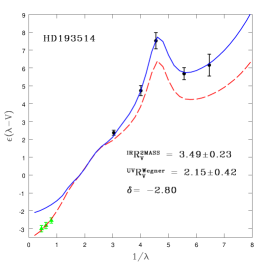
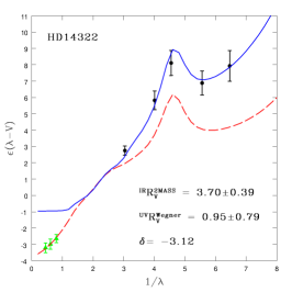
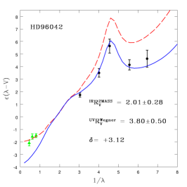
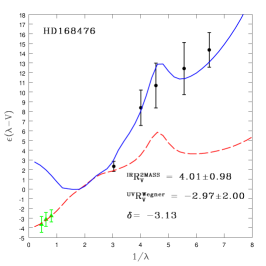
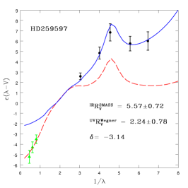
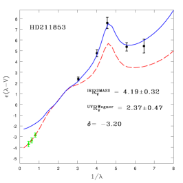
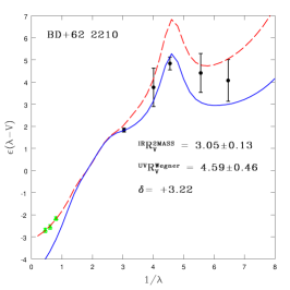
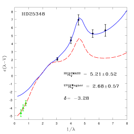
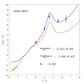
Figure 4: Extinction curves for stars listed in Table 3. The dashed line (red) is obtained using CCM law with ${}^{\rm{IR}}\!R_{V}^{\rm{2MASS}}$; the continuous line (blue) represents CCM law with ${}^{\rm{UV}}\!R_{V}^{\rm{Wegner}}$; the circular points (black) are the observed UV extinction data taken from Wegner (2002) and the triangular points (green) are 2MASS-based extinction data in the $J,H,K_{S}$ bands.

Figure 3 shows the histogram of $\delta$. The peak of the histogram around a median of $-0.64$ indicates that the number of extinction curves with ${}^{\rm{UV}}\!R_{V}<~{}^{\rm{IR}}\!R_{V}$ is higher than the one with ${}^{\rm{UV}}\!R_{V}>~{}^{\rm{IR}}\!R_{V}$ or equivalently that $R_{V}$ derived from UV spectral region tends to be smaller on average. This is an important systematic effect that deserves further study but is beyond the scope of this paper. We choose to define outliers considering the symmetric distribution around the peak: specifically, we select the outliers as the lines of sight characterized by $\delta\leq-2.0$ or $\delta\geq 1.0$. We classify them as peculiar in the sense that CCM law is not able to reproduce the whole extinction curve with a single value of $R_{V}$. Figure 4 shows these peculiar extinction curves. All 45 of them (10% of the entire sample) are listed in Table 3. In the first column we give stellar IDs; in the second column we report ${}^{\rm{IR}}\!R_{V}^{\rm{2MASS}}$ values obtained using $J,H,K$ bands from 2MASS; the third column shows the error in ${}^{\rm{IR}}\!R_{V}^{\rm{2MASS}}$; the fourth column lists ${}^{\rm{UV}}\!R_{V}^{\rm{Wegner}}$ values computed using Wegner’s (2002) data in UV; the errors in ${}^{\rm{UV}}\!R_{V}^{\rm{Wegner}}$ are given in the fifth column. The sixth column shows $\delta$ values obtained by comparing columns two and four.

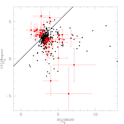
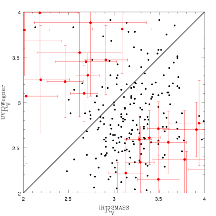
Figure 5: The comparison between the $R_{V}$ values obtained from NIR and UV extinction data. The points with error bars (red) are those for which $\delta\leq-2.0$ or $\delta\geq 1.0$. The left panel presents all data points and the right panel shows the most-crowded region in more detail.

Figure 5 presents the comparison between the $R_{V}$ values obtained from NIR and UV extinction data. There is a large scatter around the 1-to-1 relationship; however, only the 45 points with error bars shown are those which deviate from this relation significantly (according to our $\delta$ cut). Valencic, Clayton & Gordon (2004) made a similar comparison for their sample. They compared the $R_{V}$ values obtained using 2MASS photometry in IR with the $R_{V}$ values in UV obtained using International Ultraviolet Explorer (IUE). They found that 93% of their sample shows a good agreement (within 3$\sigma$) between the two values, which is consistent with our result. As opposed to Valencic et al. (2004) however, we don’t assume that our outliers must result from faulty data. We will investigate this issue in the future to see to what extent the peculiar properties come from systematic problem with the data and to what degree they are due to peculiar grain properties.

Figure 6 shows two examples of extinction curves spanning wavelength range from NIR to UV which are well fitted by the CCM law with a single $R_{V}$ value. Table 4 lists $R_{V}$ and $A_{V}$ values for all 309 of such lines of sight. Here we present only the first 15 objects. The complete table is available in the electronic version of the Journal and on the World Wide Web. In the first column we list the stellar ID, and in the second and third columns we give the coordinates. The fourth column contains $E(B-V)$ values taken from Wegner (2002); in the fifth and sixth columns we list $R_{V}$ values (obtained using all data from infrared to UV) and their errors; in the seventh column we provide $\chi^{2}/dof$ of the CCM fit; in the eighth and ninth columns we list $A_{V}$ values with their errors. There are a lot of cases for which the $\chi^{2}/dof$ is substantially less than one, which means that the errors of the individual points might have been overestimated. For this reason the $\chi^{2}/dof$ listed in Table 4 is probably a better measure of a relative rather than absolute quality of the CCM fit.

5 Conclusion

We use a $\chi^{2}$ minimization method to compute $R_{V}$ values for a sample of 436 lines of sight. We compare ${}^{\rm{IR}}\!R_{V}$ values obtained using 2MASS data with the ones computed using Wegner’s (2002) data in optical/IR. We conclude that 414 lines of sight have ${}^{\rm{IR}}\!R_{V}$ that agree using different datasets. For this final sample of 414 lines of sight we derive our $R_{V}$ values from IR and UV data assuming CCM law. We analyze the goodness of CCM fit for all lines of sight using the $\chi^{2}/dof$ statistic and test the universality of CCM law by computing $R_{V}$ values separately for the NIR and UV part of the extinction curve. We construct a catalog of $R_{V}$ and $A_{V}$ values for the 309 extinction curves with good fits to the CCM law. We divided the remaining 24% of cases into two groups, according to two main peculiarities: a) the NIR and UV extinction data points cannot be fitted well by the CCM law (14% of the entire sample), b) $R_{V}$ values are significantly different for the two spectral regions, NIR and UV (10% of the entire sample). Unless caused by faulty data, these peculiar extinction curves might come from unusual properties of dust grains. Therefore, theoretical modeling of these extinction curves (e.g., Mishchenko 1989; Saija et al. 2001; Weingartner & Draine 2001) may help us to understand the processes that modify the properties of interstellar grains.

Appendix A Transformation formulae for intrinsic colors

2MASS catalog is our primary source of IR photometry. However, since we want to use a self-consistent set of intrinsic colors over the entire wavelength range, we take the intrinsic colors from Wegner (1994) to obtain the IR color excesses. As reported in §3, the effective wavelengths of the near-infrared bands used by Wegner (1994) are $\lambda_{J}=1.25\mu m$, $\lambda_{H}=1.65\mu m$, $\lambda_{K}=2.2\mu m$ and are somewhat different from the 2MASS ones: $\lambda_{J}=1.235\mu m$; $\lambda_{H}=1.662\mu m$; $\lambda_{K}=2.159\mu m$. Well-defined color excesses come from photometry and intrinsic colors corresponding to the same wavelength. The first possibility to deal with this mismatch is to convert our adopted intrinsic colors to the 2MASS’ photometric system. To this aim, we use linear interpolation formulae:

$$(J_{2M}-V)_{0} = (H-V)_{0W}+\frac{\lambda_{J2M}-\lambda_{HW}}{\lambda_{JW}-\lambda_{HW}}[(J-V)_{0W}-(H-V)_{0W}],$$ (A1)

$$(H_{2M}-V)_{0} = (H-V)_{0W}+\frac{\lambda_{H2M}-\lambda_{HW}}{\lambda_{KW}-\lambda_{HW}}[(K-V)_{0W}-(H-V)_{0W}],$$ (A2)

$$(K_{2M}-V)_{0} = (H-V)_{0W}+\frac{\lambda_{K2M}-\lambda_{HW}}{\lambda_{KW}-\lambda_{HW}}[(K-V)_{0W}-(H-V)_{0W}],$$ (A3)

where the subscripts $2M$ indicate 2MASS, $W$ mean Wegner, and $0$ refer to the intrinsic colors. For the specific wavelengths used here we obtain:

$$(J_{2M}-V)_{0} = (J-V)_{0W}+0.025\cdot[(J-V)_{0W}-(H-V)_{0W}],$$ (A4)

$$(H_{2M}-V)_{0} = (H-V)_{0W}+0.018\cdot[(K-V)_{0W}-(H-V)_{0W}],$$ (A5)

$$(K_{2M}-V)_{0} = (K-V)_{0W}+0.073\cdot[(H-V)_{0W}-(K-V)_{0W}].$$ (A6)

For example, if we take the spectral type B1V, the color transformation will take the following form:

$$(J_{2M}-V)_{0} = (J-V)_{0W}-0.00225,$$ (A7)

$$(H_{2M}-V)_{0} = (H-V)_{0W}+0.00108,$$ (A8)

$$(K_{2M}-V)_{0} = (K-V)_{0W}-0.0044.$$ (A9)

For all relevant spectral types, we find that the color adjustments are extremely small, between 0.0001 and 0.006. Since the errors of the intrinsic colors are much bigger than the above color shifts, we neglect these corrections and use the intrinsic colors given by Wegner (1994) when analyzing 2MASS data.

It is possible to use a complementary approach and instead of adjusting intrinsic colors make a photometric transformation of 2MASS magnitudes to the Johnson’s (1966) system adopted by Wegner (2002). There are several color transformations provided by Carpenter (2001) but it is not obvious which set is the most appropriate. Independent of the transformation used the corrections to the extinction data are small, and it is safer not to apply them since the exact values and signs of those corrections depend on the very fine, unknown details of the photometric system used. This realization reinforces our decision of using 2MASS photometry with intrinsic colors by Wegner (1994) without any wavelength-related adjustments.

Figure 1: Comparison between ${}^{\rm{IR}}\!R_{V}$ values obtained using Wegner’s (2002) data with the ones computed from 2MASS’ photometry. The line represents the 1-to-1 relation and the mean errors in both coordinates are shown in the lower right corner of the plot.

Figure 2: Histograms of $\chi^{2}/dof$ for the CCM fits in IR (left) and UV (right).

Figure 3: Histogram of $\delta$ computed according to equation (10). The median of the distribution is at $-0.64$. We define outliers as the ones with $\delta\leq-2.0$ or $\delta\geq 1.0$.

Figure 6: Examples of extinction curves for which CCM law works in the entire spectral range from NIR to UV.

Table 1: Lines of sight with highly discrepant ${}^{\rm{IR}}\!R_{V}^{\rm{2MASS}}$ and ${}^{\rm{IR}}\!R_{V}^{\rm{Wegner}}$

Name	${}^{\rm{IR}}\!R_{V}^{\rm{Wegner}}$	$\sigma(^{\rm{IR}}\!R_{V}^{\rm{Wegner}})$	${}^{\rm{IR}}\!R_{V}^{\rm{2MASS}}$	$\sigma(^{\rm{IR}}\!R_{V}^{\rm{2MASS}}$)	${}^{\rm{IR}}\delta$
HD 14605	4.06	0.38	0.95	0.16	7.54
HD 39680	6.94	0.86	3.74	0.48	3.25
HD 42088	3.50	0.47	1.72	0.27	3.28
HD 44458	6.10	1.07	2.19	0.50	3.31
HD 45314	3.03	0.32	4.60	0.47	$-$2.76string
HD 46660	1.27	0.16	2.94	0.27	$-$5.32string
HD 53367	4.29	0.28	2.40	0.18	5.68
HD 53975	3.21	0.82	$-$2.23string	0.51	5.63
HD 102567	4.54	0.47	2.76	0.33	3.10
HD 155806	6.40	1.00	2.48	0.43	3.60
HD 164284	7.46	1.72	1.55	0.52	3.29
HD 170235	5.05	0.74	2.35	0.40	3.21
HD 178175	0.00	0.57	6.87	2.10	$-$3.16string
HD 192639	1.80	0.16	3.30	0.25	$-$5.05string
HD 195407	4.67	0.34	2.40	0.20	5.75
HD 200120	$-$0.20string	0.22	4.61	1.58	$-$3.02string
HD 212044	4.46	0.70	$-$0.58string	0.18	6.97
BD $56^{\circ}473$	3.38	0.35	5.02	0.49	$-$2.72string
BD $56^{\circ}586$	5.16	0.43	2.40	0.23	5.66

Note. — Columns: [1] star identification number, [2] ${}^{\rm{IR}}\!R_{V}^{\rm{Wegner}}$ values obtained using optical/NIR data from Wegner (2002), [3] error in ${}^{\rm{IR}}\!R_{V}^{\rm{Wegner}}$, [4] ${}^{\rm{IR}}\!R_{V}^{\rm{2MASS}}$ values obtained using $J,H,K$ bands from 2MASS, [5] error in ${}^{\rm{IR}}\!R_{V}^{\rm{2MASS}}$, [6] ${}^{\rm{IR}}\delta\equiv(^{\rm{IR}}\!R_{V}^{\rm{Wegner}}-^{\rm{IR}}\!\!R_{V}^{\rm{2MASS}})/\sqrt{\sigma^{2}[^{\rm{IR}}\!R_{V}^{\rm{Wegner}}]+\sigma^{2}[^{\rm{IR}}\!R_{V}^{\rm{2MASS}}]}$.

Table 2: $R_{V}$ values for the poorly fitted extinction curves [${}^{\rm{IR}}(\chi^{2}/dof)>0.28$ in the IR or ${}^{\rm{UV}}(\chi^{2}/dof)>1.6$ in the UV].

Name	${}^{\rm{IR}}\!R_{V}^{\rm{2MASS}}$	$\sigma(^{\rm{IR}}\!R_{V}^{\rm{2MASS}})$	${}^{\rm{IR}}(\chi^{2}/dof)$	${}^{\rm{UV}}\!R_{V}^{\rm{Wegner}}$	$\sigma(^{\rm{UV}}\!R_{V}^{\rm{Wegner}}$)	${}^{\rm{UV}}(\chi^{2}/dof)$
HD 7902	3.27	0.32	0.08	2.62	0.56	2.66
HD 14134	2.98	0.26	0.06	4.34	0.43	8.90
HD 14357	2.68	0.27	0.01	3.28	0.54	2.88
HD 14422	2.34	0.17	0.85	3.23	0.35	0.33
HD 17145	3.12	0.17	0.00	2.64	0.45	2.33
HD 32343	4.81	2.07	0.91	1.96	1.61	0.34
HD 37061	5.03	0.48	0.01	5.86	0.29	4.24
HD 45910	5.99	0.55	0.08	4.44	0.38	6.31
HD 46380	4.11	0.33	0.08	3.82	0.37	2.46
HD 46867	2.99	0.33	0.00	5.04	0.41	18.69
HD 50064	4.03	0.23	0.18	3.27	0.38	7.87
HD 50820	5.11	0.49	0.29	6.18	0.15	46.08
HD 59094	4.31	0.54	0.01	3.90	0.57	3.26
HD 63462	5.75	1.65	0.21	4.95	0.93	2.26
HD 73882	3.78	0.28	0.07	3.24	0.38	3.54
HD 76868	6.16	0.69	0.42	6.06	0.40	9.17
HD 93205	4.32	0.55	0.10	5.55	0.51	32.75
HD 97966	0.39	0.17	1.15	3.11	0.67	0.83
HD 101205	3.24	0.45	0.01	$-$2.17string	1.16	7.84
HD 110432	3.84	0.78	0.30	4.44	0.38	1.87
HD 147648	3.88	0.22	0.03	4.32	0.35	4.91
HD 147889	4.21	0.19	0.07	5.55	0.17	94.33
HD 147933	5.91	1.08	0.01	5.50	0.28	9.46
HD 148184	5.78	0.94	0.01	4.49	0.42	2.48
HD 149038	3.01	0.53	0.42	2.69	0.80	0.12
HD 152235	3.11	0.23	0.56	2.69	0.38	0.51
HD 152560	3.42	0.44	0.04	$-$1.05string	1.02	7.15
HD 164492	4.59	0.69	0.02	5.04	0.60	11.22
HD 168076	3.75	0.23	0.03	4.28	0.28	12.33
HD 168112	3.24	0.16	0.25	3.49	0.29	31.42
HD 168137	3.55	0.31	0.00	6.03	0.37	6.21
HD 169454	3.43	0.35	0.05	2.83	0.26	4.86
HD 172252	3.14	0.17	0.00	3.55	0.27	4.62
HD 173438	2.95	0.14	0.00	2.47	0.30	1.72
HD 177291	5.46	0.46	0.20	4.58	0.39	5.13
HD 184943	2.96	0.19	0.00	3.69	0.32	1.95
HD 186745	2.85	0.15	1.00	2.99	0.32	0.68
HD 190918	3.80	0.43	0.02	3.78	0.57	15.75
HD 190944	4.37	0.44	0.09	4.21	0.46	3.81
HD 194279	3.35	0.18	0.03	3.23	0.26	2.36
HD 198931	3.70	0.20	0.15	3.63	0.27	4.91
HD 199478	2.47	0.26	0.29	2.94	0.55	0.77
HD 200775	5.25	0.41	2.73	4.21	0.34	3.68
HD 204827	2.56	0.12	0.11	2.36	0.28	5.67
HD 206165	2.64	0.46	0.61	1.45	0.79	0.33
HD 206267	3.05	0.28	0.33	2.70	0.51	0.24
HD 206773	4.36	0.40	0.25	4.07	0.44	2.13
HD 208501	2.82	0.49	0.01	2.88	0.40	2.73
HD 209975	3.02	0.48	0.40	1.85	0.87	0.08
HD 210839	2.99	0.32	1.18	1.89	0.58	0.46
HD 217086	3.15	0.16	0.29	3.08	0.28	0.93
HD 226868	3.36	0.15	0.07	3.00	0.27	4.10
HD 228779	2.87	0.09	0.14	2.48	0.52	2.73
HD 236689	3.05	0.29	0.57	2.58	0.52	0.03
HD 236923	2.95	0.22	0.07	2.60	0.46	1.61
HD 254577	3.08	0.15	0.01	4.01	0.29	45.97
HD 262013	6.51	5.60	0.00	$-$4.57string	4.10	31.01
BD $-12^{\circ}5008$	3.17	0.12	0.01	3.21	0.20	4.77
BD $40^{\circ}4220$	3.26	0.08	0.16	3.65	0.51	5.14
BD $40^{\circ}4227$	3.22	0.10	0.00	3.08	0.18	2.09

Note. — Columns: [1] star identification number, [2] ${}^{\rm{IR}}\!R_{V}^{\rm{2MASS}}$ values obtained using $J,H,K$ bands from 2MASS, [3] error in ${}^{\rm{IR}}\!R_{V}^{\rm{2MASS}}$, [4] ${}^{\rm{IR}}(\chi^{2}/dof)$ for the best CCM fit in IR, [5] ${}^{\rm{UV}}\!R_{V}^{\rm{Wegner}}$ values obtained using UV data from Wegner (2002), [6] error in ${}^{\rm{UV}}\!R_{V}^{\rm{Wegner}}$, [7] ${}^{\rm{UV}}(\chi^{2}/dof)$ for the best CCM fit in UV.

Table 3: $R_{V}$ values for the outlier extinction curves with $\delta\leq-2.0$ and $\delta\geq 1.0$.

Name	${}^{\rm{IR}}\!R_{V}^{\rm{2MASS}}$	$\sigma(^{\rm{IR}}\!R_{V}^{\rm{2MASS}})$	${}^{\rm{UV}}\!R_{V}^{\rm{Wegner}}$	$\sigma(^{\rm{UV}}\!R_{V}^{\rm{Wegner}}$)	$\delta$
HD 2083	2.18	0.43	3.99	0.70	2.20
HD 14322	3.70	0.39	0.95	0.79	$-$3.12string
HD 21291	5.13	0.80	2.62	0.66	$-$2.42string
HD 25348	5.21	0.52	2.68	0.57	$-$3.28string
HD 30614	2.03	0.35	3.07	0.74	1.27
HD 37903	4.00	0.58	5.04	0.48	1.38
HD 46484	2.91	0.24	3.47	0.38	1.25
HD 46559	3.04	0.24	1.77	0.57	$-$2.05string
HD 46711	3.29	0.16	2.34	0.40	$-$2.21string
HD 49787	1.82	0.60	3.68	0.98	1.62
HD 54439	2.62	0.47	3.55	0.71	1.09
HD 55606	6.74	1.53	2.77	1.12	$-$2.09string
HD 61827	3.35	0.20	1.48	0.42	$-$4.02string
HD 76534	2.19	0.32	3.25	0.60	1.56
HD 96042	2.01	0.28	3.80	0.50	3.12
HD 97434	3.09	0.33	3.81	0.49	1.22
HD 113659	5.05	1.25	0.10	1.57	$-$2.47string
HD 133518	1.37	0.60	3.87	1.06	2.05
HD 135160	3.88	1.37	5.54	0.75	1.06
HD 152386	3.60	0.20	2.56	0.34	$-$2.64string
HD 152408	4.25	0.43	2.26	0.63	$-$2.61string
HD 153919	3.94	0.33	2.77	0.47	$-$2.04string
HD 155851	5.57	0.76	3.24	0.68	$-$2.28string
HD 162168	3.13	0.19	2.22	0.37	$-$2.19string
HD 163758	3.80	0.54	1.57	0.89	$-$2.14string
HD 165016	2.73	1.05	5.76	1.49	1.66
HD 168476	4.01	0.98	$-$2.97string	2.00	$-$3.13string
HD 169034	3.49	0.12	2.71	0.30	$-$2.41string
HD 185859	2.46	0.20	3.23	0.40	1.72
HD 186660	2.74	0.62	3.88	0.81	1.12
HD 186841	2.71	0.13	3.30	0.25	2.09
HD 188209	6.43	3.06	$-$4.71string	3.49	$-$2.40string
HD 191612	3.78	0.35	2.37	0.54	$-$2.19string
HD 193514	3.49	0.23	2.15	0.42	$-$2.80string
HD 194839	3.28	0.14	2.59	0.26	$-$2.34string
HD 199356	5.13	0.52	3.22	0.57	$-$2.48string
HD 206183	2.69	0.34	3.45	0.57	1.15
HD 211853	4.19	0.32	2.37	0.47	$-$3.20string
HD 217050	7.16	2.79	$-$0.82string	2.26	$-$2.22string
HD 220116	2.67	0.15	3.10	0.31	1.25
HD 228712	3.39	0.12	2.61	0.30	$-$2.41string
HD 249845	3.52	0.67	0.63	1.16	$-$2.16string
HD 259597	5.57	0.72	2.24	0.78	$-$3.14string
BD+ $41^{\circ}4064$	3.91	0.37	2.70	0.30	$-$2.54string
BD+ $62^{\circ}2210$	3.05	0.13	4.59	0.46	3.22

Note. — Columns: [1] star identification number, [2] ${}^{\rm{IR}}\!R_{V}^{\rm{2MASS}}$ values obtained using $J,H,K$ bands from 2MASS, [3] error in ${}^{\rm{IR}}\!R_{V}^{\rm{2MASS}}$, [4] ${}^{\rm{UV}}\!R_{V}^{\rm{Wegner}}$ values obtained using UV data from Wegner (2002), [5] error in ${}^{\rm{UV}}\!R_{V}^{\rm{Wegner}}$, [6] $\delta$ given by equation (10) using 2MASS data in IR and Wegner’s (2002) data in UV.

Table 4: Catalog of $R_{V}$ and $A_{V}$ values.

Name	RA(J2000)	DEC(J2000)	$E(B-V)$	$R_{V}$	$\sigma(R_{V})$	$\chi^{2}/dof$	$A_{V}$	$\sigma(A_{V})$
HD108	00 06 03.37	63 40 46.8	0.480	3.28	0.43	0.16	1.58	0.34
HD1544	00 20 05.55	62 03 58.7	0.370	2.99	0.49	0.02	1.11	0.30
HD2905	00 33 00.00	62 55 54.2	0.300	1.30	1.10	0.01	0.39	0.38
HD3901	00 42 03.90	50 30 45.1	0.085	2.36	2.24	0.11	0.20	0.28
HD4180	00 44 43.51	48 17 3.7	0.130	1.21	2.26	0.03	0.16	0.34
HD4841	00 51 25.93	63 46 52.1	0.650	3.14	0.29	0.00	2.04	0.31
HD6811	01 09 30.14	47 14 30.3	0.060	0.70	3.75	0.01	0.04	0.25
HD9311	01 33 14.01	60 41 11.2	0.360	2.99	0.49	0.00	1.07	0.29
HD10516	01 43 39.65	50 41 19.3	0.200	4.40	1.09	0.00	0.88	0.39
HD12867	02 07 53.68	57 42 45.5	0.380	2.84	0.45	0.02	1.08	0.29
HD13267	02 11 29.20	57 38 44.0	0.420	3.08	0.41	0.06	1.30	0.30
HD13900	02 17 15.56	56 53 52.9	0.380	2.89	0.47	0.04	1.10	0.30
HD13969	02 17 49.85	57 5 25.7	0.540	2.75	0.32	0.01	1.48	0.28
HD14092	02 18 41.89	56 45 40.7	0.460	2.90	0.40	0.06	1.33	0.30
HD14250	02 20 15.73	57 5 55.0	0.550	2.80	0.33	0.04	1.54	0.29

Note. — Columns: [1] star identification number, [2],[3] star coordinates, [4] $E(B-V)$ taken from Wegner (2002), [5] $R_{V}$ value obtained using NIR data from 2MASS and UV data from Wegner (2002), [6] error in $R_{V}$, [7] $\chi^{2}$ per degree of freedom derived from equation (6), [8] $A_{V}$ obtained from columns four and five, [9] error in $A_{V}$.

References

- Cardelli et al. (1989) Cardelli, J. A., Clayton, G. C., & Mathis, J. S. 1989, ApJ, 345, 245
- Carpenter (2001) Carpenter, J. M. 2001, ApJ, 121, 2851
- Fernie (1983) Fernie, J. D. 1983, A&AS, 52, 75
- Geminale & Popowski (2004) Geminale, A., & Popowski, P. 2004, Acta Astron., 54, 375
- Geminale & Popowski (2005) Geminale, A., & Popowski, P. 2005, to be published in Journal of Physics: Conference Series, Light, dust and chemical evolution, ed. R. Saija & C. Cecchi-Pestellini (astro-ph/0502480)
- Gezari et al. (1984) Gezari, D. Y., Schmitz, M., & Mead, J. M. 1984, NASA Ref. Publ, 1118
- Gezari et al. (1993) Gezari, D. Y., Schmitz, M., Pitts, P. S., & Mead, J. M. 1993, NASA Ref. Publ, 1294