Multi-object spectroscopy of low redshift EIS clusters. III. Properties of optically selected clusters

We have carried out an investigation of the properties of low redshift EIS clusters using both spectroscopy and imaging data. We present new redshifts for 738 galaxies in 21 ESO Imaging Survey (EIS) Cluster fields. We use the “gap”-technique to search for significant overdensities in redshift space and to identify groups/clusters of galaxies corresponding to the original EIS matched filter cluster candidates. In this way we spectroscopically confirm 20 of the 21 cluster candidates with a matched-filter estimated redshift $z_{MF}=0.2$. We have now obtained spectroscopic redshifts for 34 EIS cluster candidates with $z_{MF}=0.2$ (see also Hansen et al. 2002; Olsen et al. 2003). Of those we spectroscopically confirm 32 with redshifts ranging from $z=0.064$ to $0.283$. We find that: 1) the velocity dispersions of the systems range from $\sigma_{v}\leq 130\mathrm{km/s}$ to $\sigma_{v}=1200\mathrm{km/s}$, typical of galaxy groups to rich clusters; 2) richnesses corresponding to Abell classes $R\leq 1$; and 3) concentration indices ranging from $C=0.2$ to $C=1.2$. From the analysis of the colours of the galaxy populations we find that 53% of the spectroscopically confirmed systems have a “significant” red sequence. These systems are on average richer and have higher velocity dispersions. We find that the colour of the red sequence galaxies matches passive stellar evolution predictions.

1 Introduction

The evolution of galaxy clusters’ properties, as well as that of their constituent galaxies, are important issues for contemporary cosmology and astrophysics. The requirement for large samples of clusters of galaxies covering a large range in redshift has prompted systematic efforts to assemble catalogues of distant galaxy clusters (e.g. Gunn et al. 1986; Postman et al. 1996; Scodeggio et al. 1999; Gladders & Yee 2001; Gonzalez et al. 2001; Bahcall et al. 2003). The main goal behind such works is to assemble large samples of clusters with $z\gtrsim 0.5$ because at these redshifts the evolutionary effects become more significant. However, another important issue in evolutionary studies is to have a well-defined comparison sample at lower redshifts. This sample can be taken from other surveys, but it would be preferable to build it from the same survey, in order to minimize the differences in selection effects.

During the past decade a number of galaxy cluster catalogues based on optical imaging data and constructed using objective methods have become available (e.g. Postman et al. 1996; Gladders & Yee 2001; Postman et al. 2002; Bahcall et al. 2003; Goto et al. 2002). Each method uses its own combination of single passband luminosities, colour indices and galaxy position, and it is thus of great interest to compare whether the various methods detect the same systems. The comparison can be carried out along two tracks. One is to directly compare detections by different methods over the same area, and the other is to compare the general properties of the samples created by different detection algorithms (e.g. Goto et al. 2002; Kim et al. 2002; Bahcall et al. 2003; Lopes et al. 2004; Rizzo et al. 2004). Whatever the method utilized, spectroscopic follow-up is essential to confirm that the candidates are physical systems as well as to characterize their properties.

This work is part of a major on-going confirmation effort to study all EIS cluster candidates (Olsen et al. 1999a, b; Scodeggio et al. 1999). This sample consists of 302 cluster candidates with matched filter estimated redshifts $0.2\leq z_{\mathrm{MF}}\leq 1.3$ and a median estimated redshift of $z_{\mathrm{MF}}=0.5$. The cluster candidates were identified using the matched filter technique originally suggested by Postman et al. (1996). The spectroscopic confirmation of the clusters was initiated by Ramella et al. (2000), who used the multi-object spectroscopy mode at the ESO 3.6m telescope at La Silla, Chile, to obtain confirmations of intermediate redshift candidates ($0.5\lesssim z_{\mathrm{MF}}\lesssim 0.7$). They targeted six cluster candidates of which four were confirmed. Benoist et al. (2002) presented the first results for the high redshift sample ($z\gtrsim 0.8$) with confirmation of three EIS clusters.

In this work we report on a systematic spectroscopic follow-up of the low-redshift EIS cluster candidates having $z_{MF}=0.2$. The sample was drawn from candidates located in EIS patches A, B and D (Nonino et al. 1999) and consists of 68% (34 systems) of all EIS cluster candidates at this redshift. The present work follows that of Hansen et al. (2002, hereafter Paper I) and Olsen et al. (2003, hereafter Paper II). In Paper I we presented the results of a feasability study confirming five clusters in patch D of which three have $z_{\mathrm{MF}}=0.2$ and two have $z_{\mathrm{MF}}=0.3$. In Paper II we presented the follow-up of candidates in patches A and B where 9 out of 10 additional cluster candidates were confirmed. In this third paper we present the spectroscopic results for the 21 remaining systems in EIS patch D.

The paper is structured as follows: Sect. 2 gives an overview of the observations and data reduction. Sect. 3 describes the identification of systems in redshift space as well as the procedure adopted for associating the redshift groups to the EIS detections. Sect. 4 describes the properties of the spectroscopically confirmed systems including an analysis of the colour properties of the galaxy populations. In Sect. 5 we discuss our results and relate the dynamical properties to the colour properties. Finally, Sect. 6 summarizes the paper.

2 Observations and data reduction

Table 1: EIS cluster candidates in patch D with $z_{MF}=0.2$.

Field	$\alpha_{J2000}$	$\delta_{J2000}$	$\Lambda_{cl,org}$
EISJ0946-2029	09 46 12.8	-20 29 49.6	59.5
EISJ0946-2133	09 46 31.1	-21 33 24.1	30.9
EISJ0947-2120b	09 47 06.9	-21 20 55.6	43.4
EISJ0948-2044b	09 48 07.9	-20 44 31.2	42.8
EISJ0949-2145	09 49 49.4	-21 45 25.7	42.0
EISJ0949-2046	09 49 51.5	-20 46 40.6	32.8
EISJ0950-2133	09 50 46.1	-21 33 37.4	30.7
EISJ0951-2052	09 51 08.3	-20 52 23.6	32.0
EISJ0951-2026	09 51 28.9	-20 26 33.0	43.6
EISJ0951-2145	09 51 47.3	-21 45 27.1	57.9
EISJ0952-2150	09 52 46.8	-21 50 15.1	33.7
EISJ0952-2103	09 52 47.6	-21 03 02.7	34.3
EISJ0952-2144	09 52 48.6	-21 44 32.8	36.1
EISJ0952-2018	09 52 55.3	-20 18 37.6	35.4
EISJ0953-2053	09 53 05.9	-20 53 29.9	50.1
EISJ0953-2156	09 53 33.8	-21 56 10.1	35.4
EISJ0953-2017	09 53 55.5	-20 17 32.8	34.9
EISJ0955-2123	09 55 01.3	-21 23 19.6	34.0
EISJ0955-2151	09 55 04.1	-21 51 35.0	38.7
EISJ0955-2037	09 55 16.9	-20 37 04.1	36.7
EISJ0955-2020	09 55 19.8	-20 20 25.4	39.0
EISJ0956-2054	09 56 02.7	-20 54 08.6	37.3
EISJ0957-2051	09 57 07.2	-20 51 45.3	27.6
EISJ0957-2143	09 57 12.4	-21 43 13.1	40.8

The targeted cluster candidates were selected from patch D with a matched filter estimated redshift $z_{MF}=0.2$ (Scodeggio et al. 1999). In Table 1 we list the 24 selected cluster candidates. Three of these systems were already studied in Paper I as noted in the table, leaving 21 systems for the present work. The table gives: in Col. 1 the name of the field referring to the notation adopted by Scodeggio et al. (1999); in Cols. 2 and 3 the matched filter position; and in Col. 4 the $\Lambda_{cl,org}$-richness. This richness range roughly corresponds to the Abell richness classes $\leq 1$ (e.g. Postman et al. 1996).

The observations were carried out using the Danish Faint Object Spectrograph and Camera (DFOSC) mounted on the Danish 1.54m telescope at ESO, La Silla, Chile. With a field of view of $13.7\times 13.7$ square arcmins corresponding to $2.53\mathrm{Mpc}$ at $z=0.2$ (assuming $\mathrm{H}_{0}=75\mathrm{km/s/Mpc}$, $\Omega_{\mathrm{m}}=0.3$ and $\Omega_{\Lambda}=0.7$), this instrument is well-suited for MOS observations of moderate redshift clusters. The effective field that could be covered with MOS slit masks was typically $11.0\times 5.5$ square arcmins, depending on the exact configuration of galaxy positions in each field. The slit width was set to $2\arcsec$, and the slit length varied according to the extent of each galaxy. We used grism #4, giving a dispersion of $220\;\mathrm{{\AA}/mm}$, and covering a wavelength range from $3800$ to $7500\;\mathrm{{\AA}}$. However, the useful range for each spectrum depends on the exact position of the slit with respect to the chip and the intrinsic galaxy spectrum. The resolution as determined from HeNe line spectra was found to be $16.6\;\mathrm{{\AA}\;FWHM}$.

Figure 1: The distribution of completeness, the fraction of targeted galaxies to all galaxies (upper panel), and efficiency, the fraction of spectra that yielded a redshift determination (lower panel) per field.

We targeted preferentially the bright galaxies with I-magnitude, $I\leq 19.5$. The Schechter magnitude at $z=0.2$ is estimated to be $I^{*}\sim 17.5$ using an absolute Schechter magnitude of $M^{*}_{I}=-21.90$ as commonly adopted (e.g. Postman et al. 1996; Olsen et al. 1999a). The corresponding apparent magnitude was computed using the K-correction for an elliptical galaxy template spectrum from the Kinney library (Kinney et al. 1996). We thus estimate our survey to cover galaxies to 2 magnitudes fainter than the Schechter magnitude. This procedure was chosen to avoid possible biases introduced by an additional colour selection of the target galaxies. The allocated observing time allowed us to expose two slit masks for each cluster field. The exposure time for each mask was in all cases one hour. We estimate the S/N of the spectra to be in the range 5 to 15.

The data reduction was performed using the IRAF package. The CCD bias level was determined from overscan regions and subtracted. The flatfielding was carried out using the two sets of flatfields obtained immediately before and after each observation. After the basic reductions we used standard procedures to extract the spectra and to obtain redshifts by Fourier cross-correlating our spectra with standard galaxy spectra templates from Kinney et al. (1996). For the cross-correlation the template spectra were always redshifted close to the redshift under consideration. All the cross-correlation function results were visually inspected and the reliability of the peak was evaluated. Whenever a peak in the correlation function was accepted as real or possibly real, the observed spectrum was inspected and compared to the expected positions of the most prominent spectral features. We required that some features like the Ca H and K lines, the 4000 Å break, or emission lines should be identified before a determination was accepted as certain. In Paper I the reduction procedures are described in more detail.

Figure 2: The completeness (upper panel) and efficiency (lower panel) as function of magnitude as found for the cluster EISJ0953-2017. The completeness and efficiency for this cluster as computed in Table 2 correspond to the typical values as can be seen in Fig. 1.

With two slit masks per field regardless of the galaxy density we do not reach the same level of completeness in all fields, due to the variations in the local galaxy density. Therefore, we have investigated how the completeness varies from field to field. In Table 2 we summarize the spectroscopic results. The Table lists: in Col. 1 the field name; in Col. 2 the number of target galaxies; in Col. 3 the number of derived redshifts; in Col. 4 the completeness as defined below; and in Col. 5 the efficiency of obtaining redshifts (the ratio between Col. 3 and Col. 2). The completeness given in Col. 4 is defined as the ratio of observed to all galaxies brighter than $I=19.5$ within a rectangular region. The latter is defined as the smallest rectangle covering all observed galaxies and is outlined by dashed lines in Fig. 4.

In Fig. 1 we show the distributions of the completeness and efficiency. One finds that in general the completeness is $\sim 60\%$ except for three fields. This could have two reasons: (1) the galaxies are distributed such that fewer slits could fit in or (2) the field is much richer than the average field. Inspecting Fig. 4 it seems that the low completeness is probably caused by a combination of the two. The efficiency is found to cover the range between 0.53 and 0.88 with most fields having an efficiency of $\sim 80\%$.

Table 2: Summary of spectroscopic coverage for each target cluster.

Field	#targets	#redshifts	Compl.	Efficiency
EISJ0946-2133	48	33	0.50	0.68
EISJ0949-2145	45	27	0.65	0.60
EISJ0949-2046	49	37	0.19	0.75
EISJ0950-2133	50	31	0.61	0.61
EISJ0951-2052	41	32	0.76	0.78
EISJ0951-2026	48	40	0.66	0.83
EISJ0951-2145	47	28	0.17	0.59
EISJ0952-2150	54	40	0.62	0.74
EISJ0952-2103	50	42	0.14	0.84
EISJ0952-2144	50	44	0.61	0.88
EISJ0952-2018	48	39	0.52	0.81
EISJ0953-2053	52	34	0.55	0.67
EISJ0953-2156	52	41	0.62	0.80
EISJ0953-2017	47	38	0.60	0.81
EISJ0955-2123	53	41	0.67	0.76
EISJ0955-2151	48	39	0.53	0.80
EISJ0955-2037	49	26	0.69	0.53
EISJ0955-2020	34	29	0.66	0.85
EISJ0956-2054	42	32	0.62	0.76
EISJ0957-2051	39	29	0.64	0.74
EISJ0957-2143	44	36	0.68	0.81

Fig. 2 shows the completeness and efficiency as function of magnitude for the field of EISJ0953-2017, for which completeness and efficiency correpond to the typical values as found from Fig. 1. It can be seen that the completeness is very high at the brightest magnitudes but decreases to $\sim 25\%$ at about $I=19.5$. Regarding extraction of the redshifts it can be seen that the efficiency is quite high, reaching $\sim 50\%$ at $I\sim 19.5$.

In order to estimate the uncertainty of the measured redshifts we have observed several galaxies in two different masks. In total we have observed 106 galaxies twice. We use the corresponding redshift pairs to estimate the uncertainty of the individual redshift measurements. We separate the pairs in three groups: those for which we did not succeed in measuring the redshift at all, those for which the redshift could be determined in only one case and those with two redshift measurements. The first two groups cannot be used for estimating the uncertainty, but it is interesting to see that the galaxies in the first group are all fainter than $I\sim 18.8$ and in the second group they are fainter than $I\sim 17.7$. The last group consists of 49 pairs of redshifts for which the magnitudes lie in the interval $I\sim 16.1-20.0$, thus covering the entire magnitude range investigated here. For these 49 pairs we find that the standard deviation of the redshift difference between the two independent measurements is $\Delta z=0.0006$ corresponding to an uncertainty of the individual measurements of $\sigma_{z}=0.0004$. This is in good agreement with the uncertainty of the individual redshift measurements that was estimated in Paper I from the width of the peaks of the correlation function to be $\delta z=0.0005$.

3 Identification of groups in redshift space

Table 3: Redshifts measured for the individual galaxies. This table is only available in electronic form at the CDS, http://cdsweb.u-strasbg.fr/cgi-bin/qcat?J/A+A/ .

This table is only available in electronic form.

Table 4: Identified groups with a significance of at least 99% as obtained by at least one of the methods considered. Those in bold face are the ones we associate to the cluster detection as discussed in the text. When $\sigma_{v}=0$ it indicates that we measured a velocity dispersion that was smaller than the estimated error.

Cluster Field	Members	$\alpha$ (J2000)	$\delta$ (J2000)	z	$\sigma_{v}\mathrm{[km/s]}$	$\sigma_{1}$ [%]
EISJ0946-2133	7	09 46 38.5	-21 34 57.7	0.141	183	99.9
EISJ0946-2133	3	09 46 38.6	-21 33 53.3	0.153	0	99.9
EISJ0946-2133	3	09 46 25.0	-21 31 58.9	0.191	302	99.6
EISJ0946-2133	4	09 46 20.3	-21 34 56.2	0.351	562	99.7
EISJ0949-2145	4	09 49 56.2	-21 42 06.3	0.159	0	99.3
EISJ0949-2145	4	09 49 53.9	-21 44 09.3	0.184	1105	99.5
EISJ0949-2046	16	09 49 50.3	-20 46 26.8	0.143	286	99.9
EISJ0949-2046	7	09 49 57.3	-20 46 08.5	0.266	229	99.9
EISJ0950-2133	6	09 50 43.0	-21 34 20.0	0.131	126	99.9
EISJ0950-2133	3	09 50 49.8	-21 36 06.6	0.184	0	99.9
EISJ0950-2133	7	09 50 40.5	-21 35 19.7	0.235	902	99.4
EISJ0951-2052	5	09 51 00.2	-20 53 39.2	0.205	285	99.9
EISJ0951-2052	15	09 51 09.6	-20 51 56.3	0.243	833	99.9
EISJ0951-2026	4	09 51 26.7	-20 26 35.0	0.183	0	99.9
EISJ0951-2026	25	09 51 32.9	-20 27 01.1	0.242	544	99.9
EISJ0951-2145	16	09 51 48.1	-21 45 27.6	0.185	555	99.9
EISJ0951-2145	5	09 51 46.3	-21 45 48.1	0.233	488	99.7
EISJ0952-2150	6	09 52 52.3	-21 49 27.9	0.149	204	99.9
EISJ0952-2150	12	09 52 47.5	-21 49 27.9	0.183	613	99.9
EISJ0952-2150	5	09 53 07.4	-21 46 00.3	0.215	208	99.9
EISJ0952-2103	3	09 52 56.3	-21 05 11.1	0.108	124	99.4
EISJ0952-2103	3	09 53 05.5	-21 06 34.2	0.129	133	99.9
EISJ0952-2103	18	09 52 54.3	-21 03 53.6	0.236	838	99.9
EISJ0952-2144	5	09 52 54.4	-21 45 01.8	0.149	0	99.8
EISJ0952-2144	17	09 52 51.0	-21 44 45.5	0.183	595	99.9
EISJ0952-2144	8	09 53 06.8	-21 45 09.0	0.216	86	99.9
EISJ0952-2144	5	09 52 31.9	-21 42 26.7	0.234	0	99.9
EISJ0952-2144	3	09 52 31.1	-21 41 23.2	0.267	74	99.9
EISJ0952-2018	6	09 52 57.9	-20 21 34.0	0.163	0	99.9
EISJ0952-2018	14	09 53 01.7	-20 21 20.5	0.252	444	99.9
EISJ0953-2053	3	09 52 54.6	-20 52 31.3	0.204	0	99.9
EISJ0953-2053	12	09 53 06.7	-20 52 47.6	0.235	437	99.9
EISJ0953-2156	5	09 53 43.5	-21 56 20.9	0.162	1009	99.9
EISJ0953-2156	6	09 53 40.0	-21 54 52.9	0.181	0	99.9
EISJ0953-2156	5	09 53 25.3	-21 55 33.7	0.233	246	99.3
EISJ0953-2156	4	09 53 43.2	-21 54 18.2	0.330	86	99.9
EISJ0953-2017	3	09 54 06.9	-20 14 42.9	0.064	0	99.9
EISJ0953-2017	9	09 53 56.2	-20 17 26.2	0.095	195	99.9
EISJ0953-2017	3	09 54 03.8	-20 16 24.0	0.173	0	99.6
EISJ0953-2017	7	09 53 59.6	-20 16 38.7	0.282	469	99.9
EISJ0955-2123	6	09 55 12.6	-21 21 45.0	0.111	880	99.9
EISJ0955-2123	16	09 54 59.0	-21 22 19.1	0.203	739	99.9
EISJ0955-2123	3	09 54 49.2	-21 22 17.6	0.269	179	99.6
EISJ0955-2123	3	09 54 44.0	-21 21 50.9	0.415	0	99.9

Table 4: – Continued

Cluster Field	Members	$\alpha$ (J2000)	$\delta$ (J2000)	z	$\sigma_{v}\mathrm{[km/s]}$	$\sigma_{1}$ [%]
EISJ0955-2151	5	09 55 26.4	-21 52 19.9	0.105	272	99.9
EISJ0955-2151	9	09 55 00.5	-21 52 13.7	0.114	465	99.9
EISJ0955-2151	3	09 54 57.1	-21 52 55.8	0.203	752	99.2
EISJ0955-2151	8	09 55 00.8	-21 52 54.2	0.217	348	99.9
EISJ0955-2037	5	09 55 18.8	-20 34 18.2	0.234	369	99.9
EISJ0955-2037	3	09 54 57.5	-20 37 08.9	0.248	0	99.9
EISJ0955-2037	6	09 55 08.4	-20 35 30.6	0.283	221	99.9
EISJ0955-2020	8	09 55 16.0	-20 19 44.3	0.064	389	99.9
EISJ0955-2020	6	09 55 23.1	-20 19 58.1	0.104	872	99.9
EISJ0955-2020	3	09 55 32.6	-20 19 11.1	0.285	257	99.6
EISJ0956-2054	5	09 55 56.4	-20 54 23.7	0.245	200	99.9
EISJ0956-2054	17	09 56 4.4	-20 55 25.7	0.279	753	99.9
EISJ0957-2051	5	09 57 22.2	-20 52 40.5	0.148	559	99.9
EISJ0957-2051	3	09 57 13.8	-20 51 20.8	0.203	523	99.4
EISJ0957-2051	8	09 57 4.6	-20 52 49.9	0.241	387	99.9
EISJ0957-2143	3	09 57 23.9	-21 42 40.0	0.104	0	99.9
EISJ0957-2143	16	09 57 9.9	-21 44 3.5	0.202	264	99.9
EISJ0957-2143	5	09 57 19.9	-21 43 5.6	0.228	301	99.9

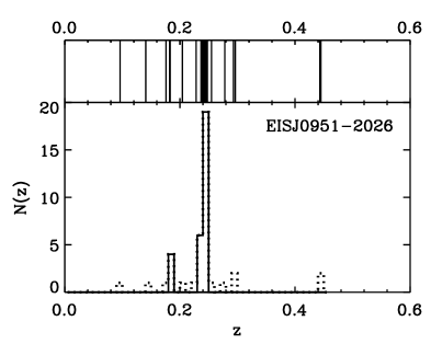
Figure 3: Redshift distributions for the 21 observed cluster fields. Note that the scale of the y-axis differs between the panels. The upper panels show bar diagrams of the measured redshifts, while the lower panels give the corresponding histograms of the redshift distributions (dotted line). The solid lines mark the detected groups.

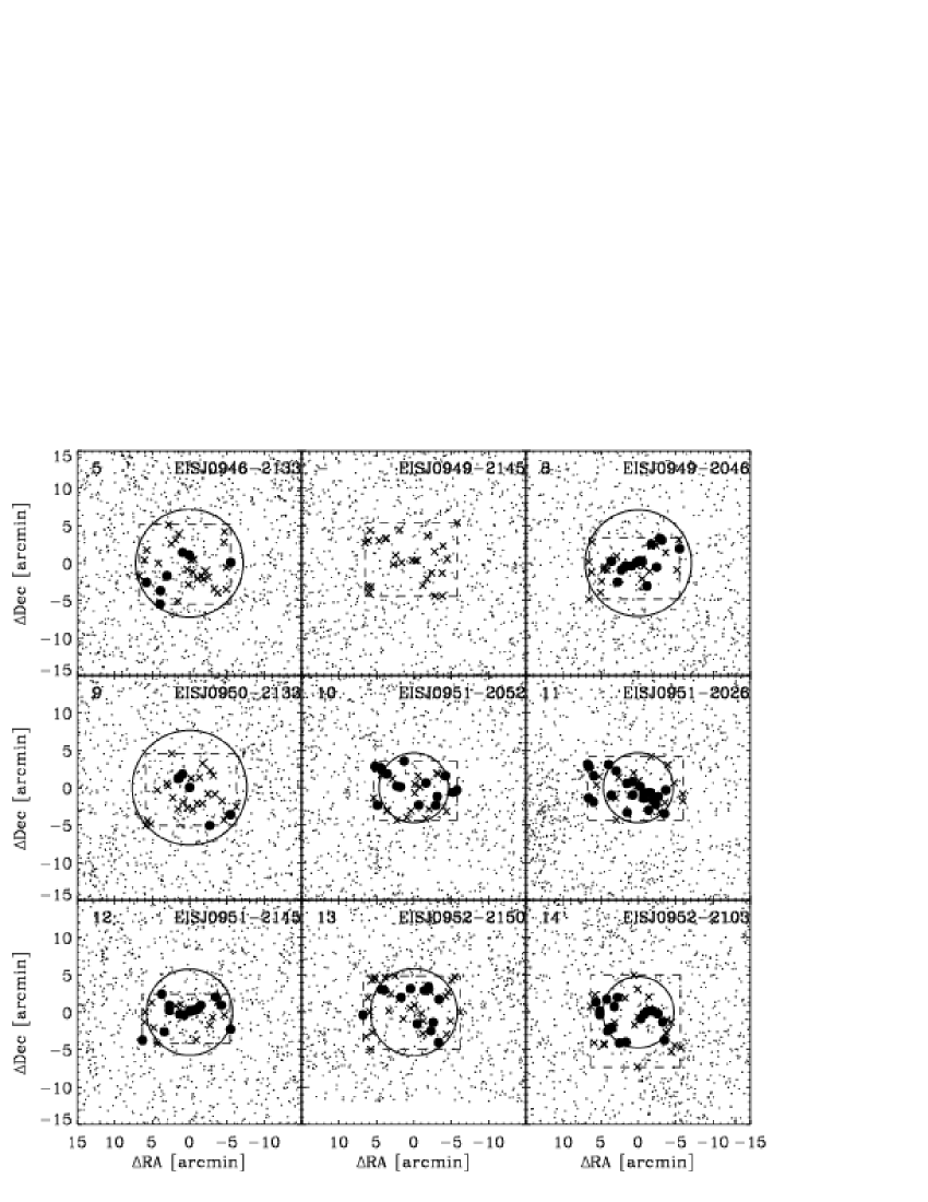
Figure 4: Projected distributions of $I\leq 19.5$ galaxies (small symbols) in each of the cluster fields. The number on the left-hand side refers to Table 5. The matched filter center of the cluster is in the center of the plots. The dashed line marks the region covered by the MOS-masks. In some cases the MOS-masks are not centered on the cluster center due to the distribution of the bright galaxies. The filled circles mark spectroscopic members of the confirmed systems, and the crosses galaxies with redshifts not belonging to the group. The large circles indicate a region of $0.5h_{75}^{-1}\mathrm{Mpc}$ at the redshift of the confirmed group.

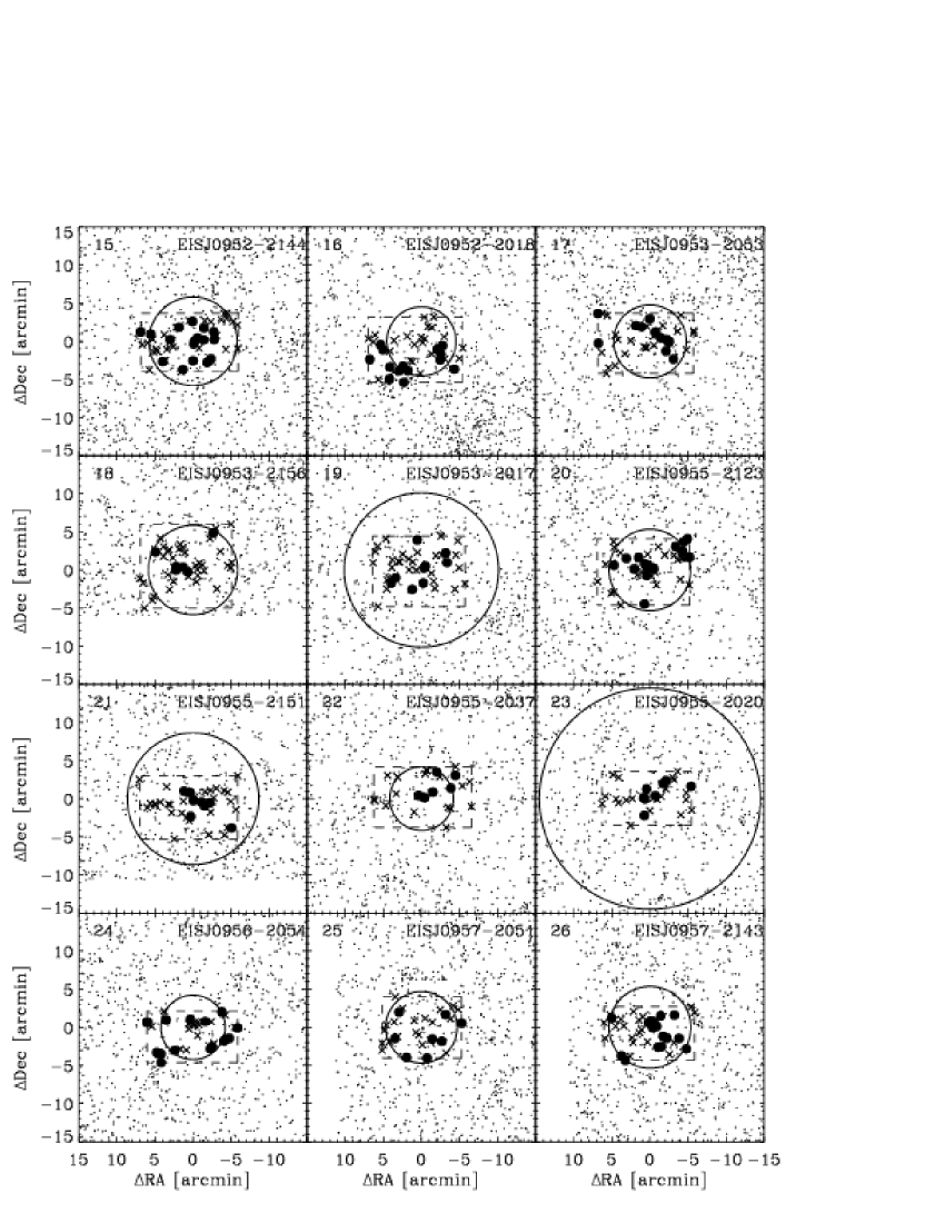
Figure 4: – Continued

We have obtained 738 redshifts for galaxies in 21 EIS cluster candidate fields. Table 3, available at the CDS, lists: in Col. 1 a running identifier for each galaxy; in Cols. 2 and 3 the right ascension and declination in J2000 for the galaxy; Col. 4 the I-magnitude from the EIS object catalogues (Benoist et al. 1999); and in Col. 5 the measured redshift. A colon (“:”) marks a measurement for which we could not identify any features to confirm the redshift, and an “e” indicates that the spectrum had emission lines.

The number of derived redshifts ranges between 26 and 44 per field. In Fig. 3 we show the redshifts for each field. The upper parts show the bar diagram of the redshifts while the lower part gives the redshift histogram with a bin size of $\Delta z=0.01$. As described in Paper II we use the “gap”-technique of Katgert et al. (1996) to identify groups in redshift space. Fig. 3 shows the identified groups as the solid histograms. We have selected a gap-size of $\Delta z=0.005(1+z)$ corresponding to $1500\mathrm{km/s}$ in the restframe. For assessing the significance of the identified groups we use the CNOC2 0223+00 catalogue (Yee et al. 2000). The significance is determined from the probability of finding a group with the same number of objects or more at the same redshift (see Olsen et al. 2003, for more details). This significance is referred to as $\sigma_{1}$.

In Table 4 we list all groups with significance larger than $99\%$ identified in each cluster field. The Table lists: in Col 1 the cluster field name; in Col. 2 the number of spectroscopic members of the group; in Cols. 3 and 4 the mean position in J2000; in Col. 5 the mean redshift of the group members; in Col. 6 the velocity dispersion corrected for our measurement accuracy. In cases where the measured velocity dispersion is smaller than the measurement error we list the value of $\sigma_{v}=0$; and in Cols. 7 the significance as defined above.

The table lists 62 significant groups, ranging between two and five groups per cluster field, having from 3 to 25 members. In many cases a single group dominates the field, with many more members than the others. In these cases, there is little ambiguity in associating this group to the matched filter detection. This is the case for 12 of 21 ($\sim 57\%$) fields. In the remaining cases the redshift distribution is more complex and consequently, the association of a group to the matched filter detection is more difficult. In other words, this is the result of the projection effects that plague the identification of clusters from a projected distribution of galaxies using a single passband.

The group associated with the matched filter detection is chosen as follows: 1) The richest group in the field, if it has a significantly larger number of members than the other groups; 2) The one closest to the EIS position, if two groups have roughly the same number of members; 3) The most concentrated group, if two groups are close to the EIS position and have almost the same number of members. Note that in all but one case (EISJ0950-2133) we associated the richest significant group with the EIS detection.

In Fig. 4 we show the projected distribution of all galaxies with $I\leq 19.5$ in the cluster regions. The solid circles mark galaxies belonging to the group associated with the EIS cluster candidate, and the crosses mark galaxies with redshifts outside the group. The large circles mark the area within $0.5h_{75}^{-1}\mathrm{Mpc}$ from the cluster center. From this analysis we find that 20 out of 21 ($\sim 95\%$) cluster candidates are confirmed as overdensities in redshift space. In one case (EISJ0949-2145), we do not consider any of the groups as representing the matched filter detection, since the number of members of the groups is small and they are spread over most of the surveyed area.

3.1 Projection effects

One of the main problems in detecting clusters from the projected galaxy distribution is the contamination along the line of sight. This effect may have two origins: one is the superposition of galaxy systems and the other the contamination by field galaxies.

As noted above, all the surveyed fields studied in the present paper contain more than one significant group in redshift space indicating that superposition effects cannot be neglected. Following Katgert et al. (1996), we consider systems to be significantly affected by superposition if the ratio of the number of member galaxies in the confirmed system to the number of members in the second largest system is smaller than two. For each confirmed system we compute this ratio and find that 8 (40%) out of the 20 systems (EISJ0946-2133, EISJ0950-2133, EISJ0953-2156, EISJ0953-2017, EISJ0955-2151, EISJ0955-2037, EISJ0955-2020, EISJ0957-2051) are likely to be affected by superposition and may have overestimated richnesses. In addition, it should be noted that these systems are also rather poor with less than 10 members and may thus also be affected by field contamination.

In the following sections we will combine the present sample with those of Paper I (3 confirmed systems out of 3 observed) and Paper II (9 confirmed systems out of 10 observed). Therefore, we have also investigated the projection effects for those systems. We find that one case (EISJ2241-3949) is likely to be affected by superposition even though it has 18 member galaxies and thus the field contamination is relatively low. Furthermore, we find four cases with less than ten members (EISJ0046-2925, EISJ2243-4013, EISJ2244-3955, EISJ2246-4012A) where only one group is identified and these systems are thus likely to be significantly contaminated by field galaxies.

In summary, we estimate that 13 out of 32 systems ($\sim 40\%$) are likely to be contaminated and care should be taken when interpreting results based on these systems.

3.2 Summary

Combining the results of the present paper with those of Papers I and II we find an overall confirmation rate of $\sim 94\%$ (32 clusters of 34 candidates) covering a region of about $\sim 9\leavevmode\nobreak\ \mathrm{square\leavevmode\nobreak\ degrees}$. This confirmation rate is consistent with the expected rate of false detecions of $\sim 1$ at $z_{MF}=0.2$ within the area considered here estimated by Olsen (2000). The results are also in good agreement with those of Holden et al. (1999), Holden et al. (2000) and Postman et al. (2002), who carried out spectroscopic follow-up of cluster candidates detected using a similar matched filter technique. Holden et al. (1999) and Holden et al. (2000) studied 9 candidates with $z_{MF}\leq 0.3$ of which they confirmed 8 and Postman et al. (2002) confirmed 13 out of 15 clusters with $z_{MF}=0.3$.

4 Properties of the detected systems

Table 5: Properties of the confirmed EIS clusters and groups. This table is also available in electronic form at the CDS, http://cdsweb.u-strasbg.fr/cgi-bin/qcat?J/A+A/ .

Id	Cluster	#mem	$z_{spec}$	$\sigma_{v}\mathrm{[}km/s]$		$\Lambda_{cl,new}$	$C$	$(V-I)_{ph}$	$\sigma_{S/N}$	$(V-I)_{sp}$	$\sigma_{spec}$	Scatter
1	EISJ0045-2923	25	0.257	$674$	${}^{+78}_{-139}$	36.4	0.54	1.800	99.9	1.800	$>99.9$	0.228
2	EISJ0046-2925	7	0.167	$970$	${}^{+88}_{-842}$	15.4	0.30	$-$	$-$	$-$	$-$	$-$
3	EISJ0052-2923	13	0.114	$615$	${}^{+72}_{-124}$	10.8	0.95	1.350	97.3	1.350	$>99.9$	0.064
4	EISJ0946-2029	28	0.111	$460$	${}^{+55}_{-93}$	32.0	0.35	1.200	99.2	1.200	$>99.9$	0.031
5	EISJ0946-2133	7	0.141	$289$	${}^{+0}_{-158}$	23.5	0.78	$-$	$-$	$-$	$-$	$-$
6	EISJ0947-2120	12	0.191	$233$	${}^{+55}_{-82}$	43.0	0.90	1.500	97.4	1.500	$>99.9$	0.065
7	EISJ0948-2044	27	0.182	$472$	${}^{+68}_{-87}$	34.9	1.04	1.500	98.0	1.425	$>99.9$	0.060
8	EISJ0949-2046	16	0.143	$311$	${}^{+84}_{-119}$	18.0	0.74	$-$	$-$	$-$	$-$	$-$
9	EISJ0950-2133	6	0.131	$27$	${}^{+178}_{-27}$	18.2	0.48	$-$	$-$	$-$	$-$	$-$
10	EISJ0951-2052	15	0.243	$1139$	${}^{+27}_{-293}$	15.4	0.90	$-$	$-$	1.575	$>99.9$	0.25
11	EISJ0951-2026	25	0.242	$703$	${}^{+72}_{-120}$	31.9	0.48	$-$	$-$	1.500	$>99.9$	0.093
12	EISJ0951-2145	16	0.185	$662$	${}^{+101}_{-127}$	50.0	0.70	1.650	98.6	$-$	$-$	$-$
13	EISJ0952-2150	12	0.183	$717$	${}^{+103}_{-208}$	30.3	0.51	$-$	$-$	1.650	$>99.9$	0.132
14	EISJ0952-2103	18	0.236	$161$	${}^{+915}_{-40}$	20.0	0.30	$-$	$-$	1.725	99.5	0.353
15	EISJ0952-2144	17	0.183	$709$	${}^{+99}_{-577}$	25.0	0.35	$-$	$-$	1.650	$>99.9$	0.043
16	EISJ0952-2018	14	0.252	$570$	${}^{+78}_{-166}$	20.0	0.37	$-$	$-$	1.500	$>99.9$	0.097
17	EISJ0953-2053	12	0.235	$488$	${}^{+125}_{-212}$	27.2	0.52	$-$	$-$	1.575	$>99.9$	0.070
18	EISJ0953-2156	6	0.181	$0$	${}^{+127}_{-0}$	30.2	0.64	$-$	$-$	$-$	$-$	$-$
19	EISJ0953-2017	9	0.095	$191$	${}^{+85}_{-54}$	10.7	0.35	$-$	$-$	$-$	$-$	$-$
20	EISJ0955-2123	16	0.203	$774$	${}^{+202}_{-279}$	41.8	0.74	1.575	91.4	1.575	$>99.9$	0.114
21	EISJ0955-2151	9	0.114	$163$	${}^{+238}_{-28}$	22.4	0.26	$-$	$-$	$-$	$-$	$-$
22	EISJ0955-2037	6	0.283	$330$	${}^{+7}_{-213}$	39.9	0.43	$-$	$-$	$-$	$-$	$-$
23	EISJ0955-2020	8	0.064	$406$	${}^{+66}_{-148}$	20.5	0.34	$-$	$-$	1.125	$99.7$	0.161
24	EISJ0956-2054	17	0.279	$962$	${}^{+114}_{-282}$	42.7	0.74	1.650	90.4	1.800	99.6	0.338
25	EISJ0957-2051	8	0.241	$483$	${}^{+65}_{-311}$	17.0	0.37	$-$	$-$	$-$	$-$	$-$
26	EISJ0957-2143	16	0.202	$325$	${}^{+61}_{-107}$	32.6	0.51	1.650	93.6	1.725	$>99.9$	0.062
27	EISJ2237-3932	35	0.244	$1210$	${}^{+108}_{-106}$	33.0	0.51	N.A.	N.A.	N.A.	N.A.	N.A.
28	EISJ2241-3949	18	0.185	$205$	${}^{+59}_{-107}$	44.8	0.78	N.A.	N.A.	N.A.	N.A.	N.A.
29	EISJ2243-4013	4	0.183	$714$	${}^{+48}_{-345}$	26.8	0.45	$-$	$-$	$-$	$-$	$-$
30	EISJ2243-4025	18	0.246	$280$	${}^{+51}_{-69}$	32.2	0.54	1.725	97.2	1.725	$>99.9$	0.037
31	EISJ2244-3955	4	0.097	$416$	${}^{+89}_{-220}$	11.2	0.30	N.A.	N.A.	N.A.	N.A.	N.A.
32	EISJ2246-4012A	6	0.150	$860$	${}^{+140}_{-395}$	21.5	0.60	$-$	$-$	$-$	$-$	$-$

In the previous section we established the existence of systems in redshift space that we consider confirmations of the EIS clusters. In this section we will further characterize the 32 confirmed galaxy overdensities (3 from Paper I, 9 from paper II and 20 from the present work) by establishing the reliability of the redshifts and velocity dispersions. To characterize the systems in more detail we also describe their richness and concentration parameters as well as determine the colours of their galaxy populations. In Table 5 we summarize the properties of the confirmed systems. The table gives: in Col. 1 a running number identifying the system; in Col. 2 the name of the cluster field; in Col. 3 the number of spectroscopic members; in Col. 4 the spectroscopic redshift; in Col. 5 the velocity dispersion with 68% bootstrap errors; in Col. 6 updated $\Lambda_{cl,new}$-richnesses as described below; in Col. 7 the concentration index as computed in Sect. 4.4; in Col. 8 and 9 the colour of the identified photometric red sequence and the confidence level as described in Sect. 4.5; in Col. 10 and 11 the colour of the red sequence of the spectroscopic members and its significance as also described in Sect. 4.5; in Col. 12 the measured colour scatter for the spectroscopic members. For three systems we do not have colour information available, so we mark the relevant entries by N.A. in the table.

4.1 Redshifts

To investigate the reliability of the measured spectroscopic redshifts for the confirmed clusters, we have compared the results from three different redshift estimators: the traditional mean redshift, the median and the biweight location (Beers et al. 1990) of the redshift of the identified systems. We find that the three estimators give consistent results with small deviations of the order $\delta z\sim 0.002$. Hence, we continue to report mean values in order to be compatible with our previously published redshifts.

Figure 5: The distribution of spectroscopic redshifts of all the confirmed systems.

In Fig. 5 we show the distribution of redshifts for all confirmed systems. We find that the average redshift of the spectroscopically confirmed systems is $\langle z\rangle=0.186$ with a standard deviation of $\sigma_{zspec}=0.058$. This is in good agreement with the matched filter estimated redshift of $z_{MF}=0.2$ given that the uncertainty in the estimated redshifts is $\Delta z=0.1$, mainly due to the spacing between redshift shells in the matched filter detection procedure.

4.2 Velocity dispersions

The velocity dispersion of galaxy systems is an important indicator of their dynamical state. In Fig. 6 we show the redshift distributions for each confirmed system. From these distributions it is clear that some systems have a small number of members, while others show signs of substructure. Therefore, it is important to determine the velocity dispersion using an estimator that is robust both for small samples and with respect to outliers. Beers et al. (1990) investigated the problem in detail and suggested the use of the biweight scale or gapper estimators.

We have compared the estimates of the velocity dispersion for our systems using these two estimators as well as the traditional standard deviation. In general, the velocity dispersions estimated by the different methods are consistent with the differences of the order $\lesssim 50\mathrm{km/s}$, much smaller than the bootstrap-estimated errors. However, in two cases the biweight estimator gives significantly smaller values than the other two (though with large errors and still the values agree within the errors). These two cases are EISJ0952-2103 (panel 14 of Fig. 6) and EISJ0955-2151 (panel 21) with the traditional standard deviation giving estimates that are significantly higher.

Inspecting the redshift distribution of EISJ0952-2103 we find that the 18 members split into three groups containing one, five and twelve members, respectively. We find that the biweight estimator reflects the velocity dispersion of the largest, and most concentrated group, while the other methods are more sensitive to the outlying members. The large error given in Table 5 probably reflects the presence of the outliers.

The other case is EISJ0955-2151 (panel 21) with only 9 members, one being an outlier, which explains the large discrepancy reported above and the large error in Table 5. It is worth emphasizing, that this system is one of those we, in Sect. 3, found to be affected by projection effects.

Inspecting Fig. 6 we also find outliers in panels 15, 20 and 25. However, in these cases the different velocity dispersion estimates are not as discrepant as in the aforementioned cases, but large errors, comparable to those discussed above, reflect the presence of outliers.

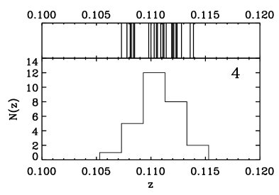
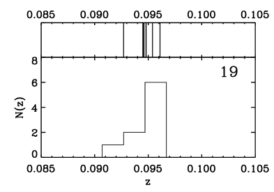
Figure 6: Detailed redshift diagrams for all spectroscopically confirmed systems. The identification numbers in each panel refer to Table 5. Upper panels show a bar diagram of the redshifts of cluster members. The lower part shows the redshift histogram with a bin size of $\Delta z=0.002$.

Hereafter, we adopt the biweight method to compute the velocity dispersions listed in Col. 5 of Table 5 with 68% bootstrap errors. The distribution of these velocity dispersions (solid line) is shown in Fig. 7. This distribution is compared to those of Fadda et al. (1996) and Zabludoff et al. (1990), which will be discussed in Sect. 5. As seen from this figure and Table 5 we find systems with very low velocity dispersions. In particular, the clusters EISJ0950-2133 (panel 9) and EISJ0953-2156 (panel 18) have implausibly low velocity dispersions, possibly indicating severe undersampling.

Figure 7: Distribution of velocity dispersions (solid line) compared with those of Fadda et al. (1996) – dotted histogram – and those of Zabludoff et al. (1990) – triple dot-dashed histogram.

4.3 Richness

The matched filter algorithm also provides a measure of the richness ($\Lambda_{cl}$) for the cluster candidates based on the estimated redshifts, where the $\Lambda_{cl}$-richness is equivalent to the number of $L^{*}$-galaxies contributing to the matched filter signal of a particular detection. This computation depends on the apparent Schechter magnitude and angular extent of the cluster, which at these redshifts vary rapidly. Therefore, even though the spectroscopic and estimated redshifts are in good agreement we have to recompute the cluster richness using the assigned spectroscopic redshift. The new richness values ($\Lambda_{cl,new}$) are listed in Table 5 and compared with the original estimates ($\Lambda_{cl,org}$) in Fig. 8. In general the new richnesses are smaller than the original ones. This is in good agreement with the, on average, lower redshift relative to the $z_{MF}$ estimate since the expected apparent Schechter magnitude is now brighter and thus the observed cluster luminosity corresponds to fewer $L^{*}$-galaxies. The lower redshift also causes a larger region to be used for the richness measurement, but the added luminosity from those large cluster-centric distances is small.

Figure 8: The relation between the original matched filter estimated $\Lambda_{cl,org}$ richnesses and the new ones, $\Lambda_{cl,new}$. The solid line marks $\Lambda_{cl,org}=\Lambda_{cl,new}$.

Figure 9: The distribution of $\Lambda_{cl,new}$-richnesses.

Finally, in Fig. 9 we show the distribution of $\Lambda_{cl,new}$-richnesses that covers the range $10\lesssim\Lambda_{cl,new}\lesssim 50$. This range corresponds to Abell richness class $\leq 1$, typical of poor galaxy clusters. This is not surprising considering the relatively small volume surveyed for clusters at the low redshift range considered here.

4.4 Concentration

Using the definition by Butcher & Oemler (1984) we have computed concentration indices for all the clusters. The concentration index is defined as $C=\log\left(R_{60}/R_{20}\right)$, where $R_{n}$ is the radius encircling n% of the galaxies. Butcher & Oemler found that, in the local Universe, clusters with $C\gtrsim 0.4$ were centrally concentrated and dominated by ellipticals, while those with $C\sim 0.3$ are closer to uniform-density spheres and would be dominated by spirals.

Figure 10: The distribution of concentration indices for the confirmed systems (solid line) compared with the distribution from Butcher & Oemler (1984) given by the dashed histogram.

We compute the concentration index based on the background corrected galaxy counts within $2h_{75}^{-1}\mathrm{Mpc}$ from the cluster center with $I\leq I^{*}(z)+2$, where $I^{*}(z)$ is the expected I-band Schechter magnitude at the redshift of the cluster (see Sect. 2). The background correction is based on galaxies with magnitudes in the same range and clustercentric distance between $2h_{75}^{-1}\mathrm{Mpc}$ and $3h_{75}^{-1}\mathrm{Mpc}$. The computed concentration indices are given in Table 5 and their distribution (solid line) is shown in Fig. 10. For comparison, the distribution of concentration indices found by Butcher & Oemler is also shown and will be discussed in more detail in Sect. 5. The EIS systems cover a broad range of concentration indices from “ uniform” to highly concentrated systems.

4.5 Colour of the galaxy population

4.5.1 Detection method

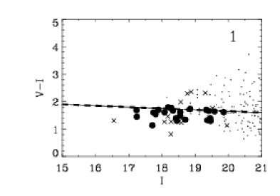
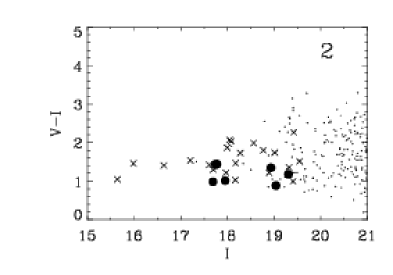
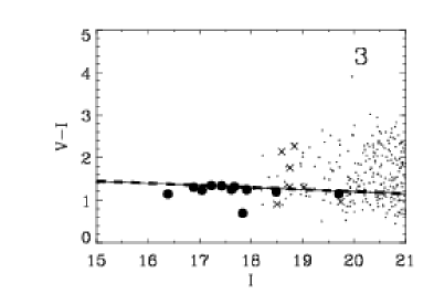
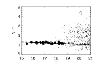
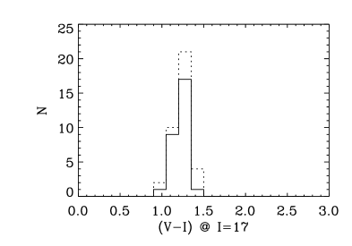
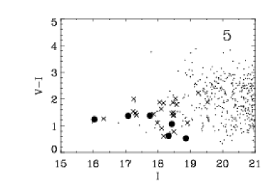
Figure 11: For each cluster we show 3 diagrams with the cluster identification number indicated in the first one. The first diagram is the colour-magnitude diagram for all galaxies within $0.75h_{75}^{-1}\mathrm{Mpc}$ from the cluster center (dots). On top of that we mark by solid circles the spectroscopic members of the confirmed group and by crosses the remaining galaxies with redshifts. The solid line is the locus of the red sequence detected from the spectroscopic members and the dashed line is the one detected in the photometric analysis. In both cases we only show the line if we consider the sequence significant (see the text for details). The second plot is the “tilted colour histogram” for the galaxies with $I\leq 19.5$ in the same region statistically corrected for the background contribution. The last panel is the “tilted colour histogram” for the spectroscopic members (solid line) and for all galaxies with a redshift (dotted line).

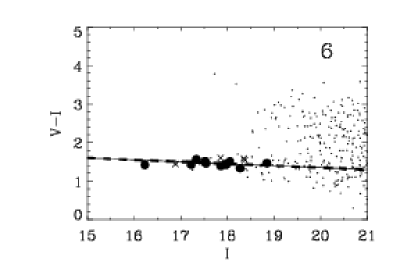
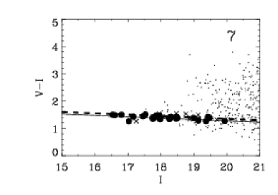
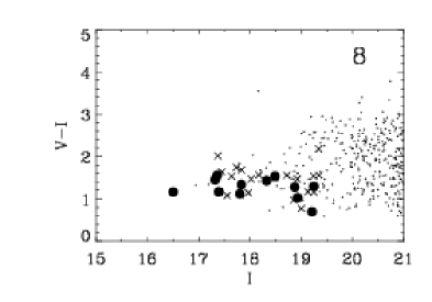
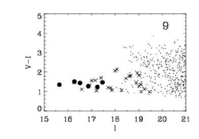
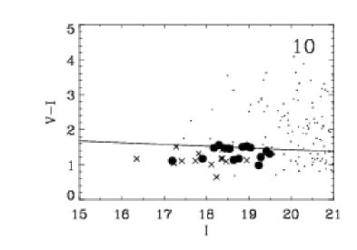
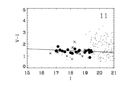
Figure 11: – Continued

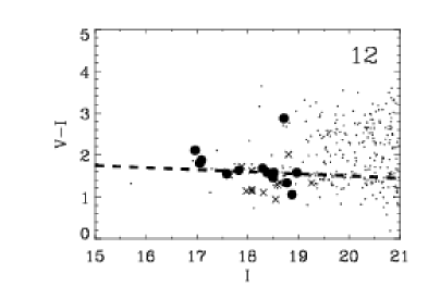
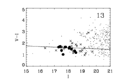
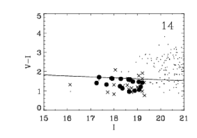
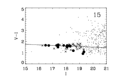
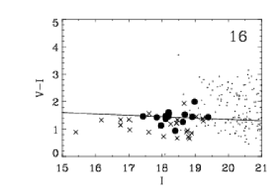
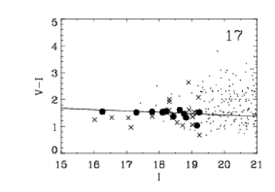
Figure 11: – Continued

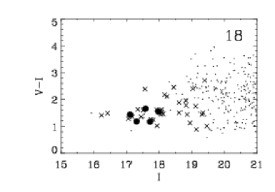
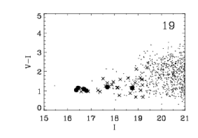
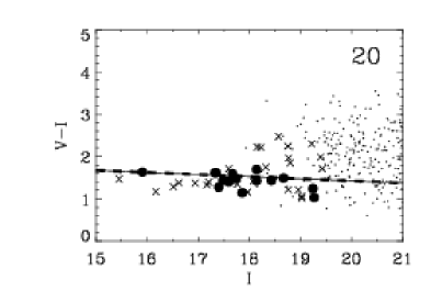
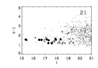
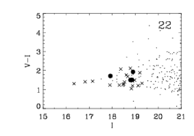
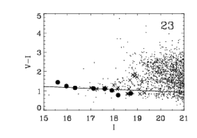
Figure 11: – Continued

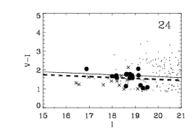
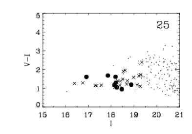
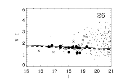
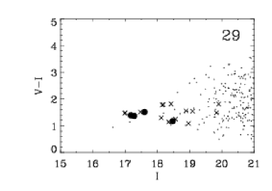
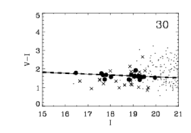
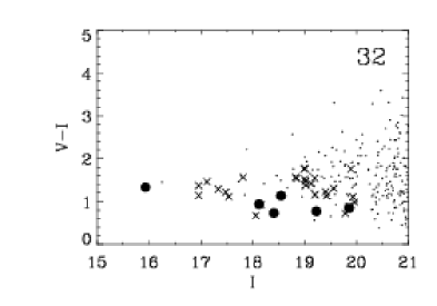
Figure 11: – Continued

Another important characteristic of a galaxy cluster is the colour properties of its population. In particular, the colour-magnitude diagram of cluster members normally reveals the presence of a narrow sequence of bright, early-type galaxies known as the “red sequence” (e.g. Gladders et al. 1998; Stanford et al. 1998; Holden et al. 2004; López-Cruz et al. 2004). The presence of this colour-magnitude (CM) relation serves as unambiguous evidence for the presence of a real physical system. Furthermore, its characteristics, such as colour, slope and scatter, have been extensively used to constrain galaxy evolution models (e.g. Gladders et al. 1998). While most of the previous studies focused on relatively rich systems, the presence of red sequences in very poor clusters and groups has also been reported (e.g. Andreon 2003).

The properties of the colour-magnitude relation are found to be very homogeneous, even though they evolve with redshift (e.g. Aragón-Salamanca et al. 1993; Stanford et al. 1998). Below we use this fact and the measured slope for clusters at redshifts close to the ones being considered here as the basis for an objective method for detecting CM relations.

For 29 of the 32 systems analysed here, $V$-band images were also available, thus allowing us to construct and investigate the CM diagram of the “cluster” members. The $(V-I)\times I$ CM diagrams were constructed considering galaxies within a radius of $0.75h_{75}^{-1}\mathrm{Mpc}$ and are shown in Fig. 11. For each system: 1) the left panel gives the aforementioned colour-magnitude diagram for galaxies (dots) brighter than $I=21$; filled circles indicate spectroscopically confirmed members and crosses other galaxies with measured redshifts. Also shown in this panel are the best-estimated loci characterizing the so-called red sequence (see below) as determined from the photometric data alone (dashed line) and that obtained considering only the confirmed spectroscopic members (solid line); 2) the middle panel shows the background-corrected colour distribution of galaxies brighter than $I=19.5$ within the same radius. The background correction is estimated from the colour distribution of galaxies lying between radii $2h_{75}^{-1}\mathrm{Mpc}$ and $3h_{75}^{-1}\mathrm{Mpc}$; and 3) the right panel shows the colour distribution of spectroscopic members (solid histogram) and that of all galaxies with measured redshifts (dotted histogram).

From these diagrams it is clear that some of the clusters do have a well-defined red sequence, while for others the red sequence is either poorly defined or completely absent. Here we use the properties of the CM relation mentioned above to develop an objective method for determining its presence and properties.

As mentioned above, the red sequence consists of early-type cluster galaxies. Therefore, to identify the presence of a red sequence and thus distinguish between localized density enhancements and physically bound systems, one would require both morphological information and complete spectroscopic data. In the present work we do not have morphological data nor complete spectroscopic data and therefore we carry out a statistical analysis to identify red sequences in the colour distribution of galaxies in the cluster fields using the following method. First, we build a “tilted colour histogram”, counting galaxies within slices of a given width and characterized by a slope taken to be comparable to that typically observed for the CM relations of nearby clusters. We then construct two such histograms with a relative shift of half a bin width. This is done in order to avoid splitting a sequence between two bins, thereby artificially decreasing its significance. To obtain the colour histogram only for the cluster galaxies, the histograms are background corrected, as described below. We determine the colour of the red sequence by separately analyzing both histograms. First, we identify the highest peak considering only those that are narrower than a certain value, taking into account the fact that the scatter around the CM relation in nearby clusters is very small ($\leq 0.1\mathrm{mag}$, e.g. López-Cruz et al. 2004). Next, based on simulations, we compute the confidence level of the peaks and assign the colour of the most significant peak to be that of the red sequence.

We apply this method to two datasets. First, we consider all available photometric data, which has the advantage of good statistics but is susceptible to projection effects possibly leading to contamination by non-cluster members, thereby diluting a possible red sequence. Then, we consider the spectroscopic data. While these are not affected by projection effects, the statistics are usually poor due to both the low richness of the systems being analysed and the incompleteness of the spectroscopic data. There may also be false detection of a red sequence due to incompleteness/selection effects.

In the analysis described below and illustrated in the middle and right panels of Fig. 11 we use the following parameters. The bin width is chosen to be $\Delta(V-I)=0.15\mathrm{mag}$. Because of the tilted nature of the histograms we arbitrarily define the center of the bins at $I=17$ and in the range from $(V-I)=-0.075$ and $(V-I)=2.85$. We adopt a slope of $-0.05$ as found by López-Cruz et al. (2004) for the $(B-R)\times R$ CM relation at $z\sim 0.05$. The $(B-R)$ at that redshift roughly corresponds to $(V-I)$ at $z\sim 0.2$. We restrict the red sequence colours to be in the range $1.0\leq(V-I)\leq 2.0$. This colour range was chosen to avoid the tails of the colour distributions, where poor statistics may artificially increase the peak significances. Furthermore, it is well-matched with the colours expected for elliptical galaxies at these redshifts (e.g. Bruzual & Charlot 1993). We only consider peaks narrower than $0.3\mathrm{mag}$. This choice is rather conservative since the estimated uncertainties of the $(V-I)$ colour at the faintest end considered is $\sigma_{(V-I)}\sim 0.04$ (Prandoni et al. 1999).

4.5.2 Photometric data

In this case the “tilted colour histogram” is constructed for galaxies brighter then $I=19.5$ within the area inside a radius of $0.75h_{75}^{-1}\mathrm{Mpc}$, hereafter referred to as the cluster area. The background contribution is estimated from the “tilted colour histogram” of galaxies in the same magnitude range but at a distance ranging from $2h_{75}^{-1}\mathrm{Mpc}$ to $3h_{75}^{-1}\mathrm{Mpc}$ and then scaled to the cluster area. For bins for which the expected field contribution is larger than the number of galaxies in the cluster area, we set the number of cluster galaxies to zero. In order to compute the significance of the identified peaks we use the signal-to-noise ratio ($S/N=N_{cl}/\sqrt{N_{tot}+N_{bkg}}$). Here $N_{cl}$ is the number of cluster galaxies in the bin, $N_{tot}$ is the number of galaxies in the bin in the original histogram before field correction and $N_{bkg}$ is the expected number of background galaxies in that bin for the cluster area.

In order to quantify the significance ($\sigma_{S/N}$) of a given $S/N$ we have carried out a series of simulations. For each measured cluster redshift we have selected 1000 random positions within our $(V-I)$ galaxy catalogue and constructed similar “tilted colour histograms” for those positions. From these histograms we construct the distribution of the measured $S/N$ and determine the probability of finding a peak with a similar $S/N$ as the one found for the cluster. Since we limit ourselves to a quite narrow colour range ($1.0\leq(V-I)\leq 2.0$), the field contribution is roughly constant and thus we do not separate the significances by colour. In Fig. 12 we show the distribution of the measured $S/N$ for three different redshifts. It is clear that one cannot rely on simply taking the same $S/N$ threshold for all redshifts. This is mainly due to the larger sky area for the nearer clusters. In order to determine the significance for a given system we use the simulations carried out using the same redshift and determine how frequently a peak with similar or larger $S/N$ occur in the field samples. The significance is computed as this frequency subtracted from unity. We define the threshold for considering a red sequence real to be $\sigma_{S/N}\geq 90\%$. In the middle panels of Fig 11 we show that of the two histograms with the highest peaks.

Figure 12: Distribution of red sequence S/N values for 1000 random galaxy samples for three different redshifts.

4.5.3 Spectroscopic data

The “tilted colour histograms” of the spectroscopic members do not need any background subtraction. The significance of the peak is assessed by constructing random galaxy samples. For each confirmed system we select 1000 galaxy samples from the entire galaxy catalogue with the same size as the confirmed system. The “tilted histograms” of these randomly selected galaxy samples are analyzed in the same way as the data and we determine how frequently we encounter a peak with at least the same number of galaxies as found in the peak of the data. The definition of the significance, $\sigma_{spec}$, is analagous to that above. In this case, we define the threshold for considering a red sequence real to be $\sigma_{spec}\geq 99\%$. The histograms with the highest peaks are shown in the right panels of Fig 11.

4.5.4 Results

From the application to the photometric data we find 10 systems ($\sim 35\%$) that show signs of a red sequence, while we identify 17 systems ($\sim 55\%$) when the spectroscopic sample is used. Interestingly, all but one of the systems for which a red sequence was identified from the photometric data are confirmed by the spectroscopic analysis. Moreover, the colours determined by the two methods yield comparable results. The colours obtained for the red sequences (see Fig. 18 below) are consistent with the passive evolution model by Bruzual & Charlot (1993). The only system which was not confirmed by the spectroscopic analysis is EISJ0951-2145 (#12) which is one of the cluster fields with the lowest completeness (0.17) in terms of targeted galaxies.

On the other hand, we find 8 systems where a red sequence was found in the spectroscopic sample but not from the photometric sample alone. Curiously, in only one case (EISJ0955-2020, #23) have we found, in Sect. 3, that the system was significantly affected by projection effects.

In summary, a total of 18 systems show evidence of having a red sequence. We find 10 systems from the photometric data alone and 17 from the spectroscopic analysis with 9 systems being in common.

For the systems with red sequences detected from the spectroscopic analysis we computed the scatter of the galaxy colours using an iterative sigma-clipping method. The scatter is given in Col. 12 of Table 5 and shown in Fig. 13 (solid line). It ranges from 0.031 to $0.35\;\mathrm{mag}$. For comparison, we also show the distribution of scatter measured in (B-R) by López-Cruz et al. (2004) scaled to the same total number of clusters. This will be discussed in more detail below.

Figure 13: Distribution of the measured scatter around the red sequences (solid line) compared to that of López-Cruz et al. (2004) (dashed line).

4.6 Comparison with other authors

In Fig. 7 we compare the normalized distributions of velocity dispersions of the EIS systems (solid line) with those of the cluster samples considered by Fadda et al. (1996) (dotted line) and Zabludoff et al. (1990) (dashed line), both drawn from the Abell cluster catalogue. Both of these samples cover roughly the same redshift range $z\lesssim 0.15$. The Fadda et al. sample includes 172 clusters with richness as poor as $R=-1$, while that of Zabludoff et al. consists of 65 clusters most of which have richness $R\geq 1$. From the figure we find that the EIS systems span about the same range of velocity dispersion as the other samples, but apparently with a larger fraction of low velocity dispersion systems. Applying the Kolmogorov-Smirnoff test, we find that this difference is significant with only a small probability that our sample is drawn from the same parent population as the others.

The distribution of richness is shown in Fig. 9. Unfortunately no similar samples are available for comparison. Instead, we compare, in Fig. 14, the relation between velocity dispersion and richness with that determined by Bahcall et al. (2003). In the figure the solid line shows the relation obtained by Bahcall et al., with the dashed lines indicating the estimated uncertainty interval. This relation was derived using 20 well-sampled clusters drawn from the Sloan Digital Sky Survey data by a matched filter algorithm. From the figure we find that, except for a few cases at the low richness end, the EIS systems populate the same region of the plot. However, considering all systems, we find only a weak correlation between these global parameters, perhaps indicating that effects of projection and outliers contaminate the measurements of the richness and velociy dispersion. We point out that, in their analysis, Bahcall et al. (2003) only considered richer systems ($\Lambda\geq 30$).

In Fig. 10 we show the distribution of concentration indices for our clusters and for those of Butcher & Oemler (1984). It can be seen that the EIS sample covers a larger range of concentration indices than that of Butcher and Oemler. We find a mean concentration of $\langle C\rangle_{EIS}=0.56$ with a standard deviation of 0.21, larger than the one found by Butcher & Oemler ($\langle C\rangle_{BO}=0.47$ with a standard deviation of 0.10), indicating that our sample includes more concentrated systems.

Figure 14: The relation between $\Lambda_{cl,new}$ and $\sigma_{v}$ for the 31 confirmed systems with a measured velocity dispersion. The solid line marks the scaling relation derived by Bahcall et al. (2003) with the dashed lines marking its uncertainty.

Figure 15: The colour dispersion as function of redshift for all systems with a red sequence identified in the spectroscopic analysis.

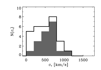
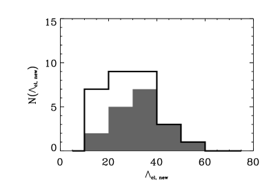
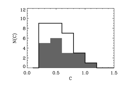
Figure 16: Global properties of the red-sequence systems (gray region) compared with those of the entire sample (solid line). The left panel shows the distribution of velocity dispersion, the middle panel that of richness and the right panel that of concentration index.

In Fig. 13 the distribution of the scatter about the CM relation for the 17 systems having a red sequence detected using the spectroscopic sample is shown and compared to that of López-Cruz et al. (2004). Considering all our systems we find a mean scatter of $0.13\pm 0.10$, where the error is the standard deviation. Discarding the four systems with measured scatters larger than $0.2\mathrm{mag}$ we obtain a mean scatter of $0.079\;\mathrm{mag}$, in excellent agreement with the results of López-Cruz et al. (2004), who found a scatter of $0.074\pm 0.026\;\mathrm{mag}$. With the exception of one of the four outlying systems all have highly complete spectroscopic data. In Fig. 15 we show the measured scatter as function of redshift. It can be seen that the four outlying systems are all found at redshifts $z\geq 0.23$. All the systems but the one with incomplete spectroscopic data have concentration indices $C>0.5$, which corresponds to concentrated systems using the definition of Butcher & Oemler (1984). A possible interpretation for this larger scatter for these higher redshift systems is that they have bright blue cluster members, reminiscent of the Butcher-Oemler effect (Butcher & Oemler 1984). The onset of this is thought to happen at redshift $z\sim 0.1$ with the fraction of blue galaxies increasing from $f_{B}\sim 0.03$ to $f_{B}\sim 0.25$ at $z=0.5$ in compact, concentrated clusters. Without morphological information, the origin of this scatter cannot be determined.

5 Discussion

To better understand the relation between the existence of a red sequence and the global properties of the galaxy cluster/ group, here we focus on the 17 clusters with red sequences and compare their properties to those found for the entire sample in Fig. 16. The left panel gives the distribution of velocity dispersion, the middle panel that of richness and the right panel that of concentration index. In all panels the distribution for the entire sample is shown (solid line), while that for the red-sequence systems are represented by the gray histogram. From the figure, we conclude that the red sequences are found in rich, high-velocity dispersion systems, but their existence is independent of the concentration.

In Fig. 17 we show the richness-velocity dispersion relation of Bahcall et al. (2003), discussed in the previous section, considering only the red-sequence systems. Except for two low-richness systems, all of them fall within the region indicated by the Bahcall et al. relation. The correlation found for the 15 systems with $\Lambda_{cl,new}\geq 20$ is 0.29, with a fitted relation of $\sigma_{v}=73\Lambda_{cl,new}^{0.55}$.

Figure 17: The relation between $\Lambda_{cl,new}$ and $\sigma_{v}$ for the 17 systems for which we identify red sequences from the spectrocopic analysis. The solid line marks the scaling relation derived by Bahcall et al. (2003) with the dashed lines marking its uncertainty.

Finally, in Fig. 18 we compare our measured red sequence colours as a function of redshift with those predicted by two different models. The two models represent passively evolving (thick line) and non-evolving (thin line) elliptical galaxies. The passive evolution model is based on the model by Bruzual & Charlot (1993) with a formation redshift $z_{f}=10$ with a short starburst followed by passive evolution. The colours for the non-evolving elliptical galaxy are computed from the composite elliptical spectrum from Kinney et al. (1996). The data points seem to be consistent with the passive evolution model, as has also been found by previous work (e.g. Aragón-Salamanca et al. 1993; Gladders et al. 1998; Stanford et al. 1998; Olsen et al. 2001). The scatter around the passive evolution model is computed to be $0.14$, comparable to the bin width utilized to determine the colour of the red sequence.

Figure 18: The relation between the redshift of the systems and the colour of the red sequence. The number 2 indicates that there are two symbols falling almost on top of each other. The lines mark the no-evolution (thin line) and the passive evolution (thick line) predictions.

6 Summary

In this paper we report new redshifts for 738 galaxies in the field of 21 low-redshift ($z_{MF}=0.2$) candidate clusters drawn from the EIS candidate cluster sample. These data were used to search for overdensities in redshift space, thus confirming the presence of a bound group/cluster of galaxies in the direction of candidates identified by the matched-filter analysis. The photometric and spectroscopic data available for the 20 new confirmed clusters out of 21 candidate systems, as well as those listed in the previous papers of this series (Hansen et al. 2002; Olsen et al. 2003), were used to compute the properties of these systems and member galaxies. Our main results can be summarized as follows:

1. For 32 (94%) of 34 systems considered we identify significant density enhancements in redshift space. We find that the measured redshifts are in the range $0.06\leq z\leq 0.28$, with a mean value of $z=0.18$. This is in excellent agreement with the redshift estimated by the matched filter technique.

2. The systems have a broad range of properties. The velocity dispersions range from small groups ($130\mathrm{km/s}$) to clusters ($1200\mathrm{km/s}$), the richness tends to be low and the concentration varies from uniform, typical of spiral-dominated systems to highly concentrated, typical of early-type dominated systems. The fact that the systems are predominantly poor is not surprising given the relatively small volume of space probed by the survey.

3. We estimate that 13 out of the 32 systems may suffer from projection effects either due to other superposed galaxy systems along the line-of-sight or to field galaxies, which may impact the calculation of the system’s global properties and explain the weak correlation observed between velocity dispersion and richness.

4. We find that 17 (60%) out of 29 systems with both photometric and spectroscopic data available show evidence of a red sequence in the colour-magnitude diagram, with colours consistent with those predicted from passively evolving stellar populations. Only one system with a detected red sequence using photometric data was not confirmed when only spectroscopic members were considered.

5. The systems where red sequences have been detected tend to have higher velocity dispersions and richnesses than those without. However, these systems seem to be independent of the concentration index.

The presence of a red sequence is consistent with the interpretation that we have detected bound systems containing elliptical galaxies that obey a scaling mass-metallicity relation which gives rise to the observed CM-relation. Therefore, these results taken together with the detection of density enhancements in redshift space provide further evidence that the systems detected by the matched-filter technique at z=0.2 are nearly all real. Extending the sample of measured redshifts would greatly help in further characterizing these systems, typically at the low end of the Abell richness.