The Molecular ISM of Dwarf Galaxies on Kiloparsec Scales: A New Survey for CO in Northern, IRAS-detected Dwarf Galaxies

Abstract

We present a new survey for CO in dwarf galaxies using the ARO Kitt Peak 12m telescope. This survey consists of observations of the central regions of $121$ northern dwarfs with IRAS detections and no known CO emission. We detect CO in $28$ of these galaxies and marginally detect another $16$, increasing by about 50% the number of such galaxies known to have significant CO emission. The galaxies we detect are comparable in stellar and dynamical mass to the Large Magellanic Cloud, although somewhat brighter in CO and fainter in the FIR. Within dwarfs, we find that the CO luminosity, $L_{CO}$, is most strongly correlated with the $K$-band and the far infrared luminosities. There are also strong correlations with the radio continuum and $B$-band luminosities, and linear diameter. Conversely, we find that FIR dust temperature is a poor predictor of CO emission within the dwarfs alone, though a good predictor of normalized CO content among a larger sample of galaxies. We suggest that $L_{CO}$ and $L_{K}$ correlate well because the stellar component of a galaxy dominates the midplane gravitational field and thus sets the pressure and density of the atomic gas, which control the formation of H₂ from H I. We compare our sample with more massive galaxies and find that dwarfs and large galaxies obey the same relationship between CO and the 1.4 GHz radio continuum (RC) surface brightness. This relationship is well described by a Schmidt Law with $\Sigma_{RC}\propto\Sigma_{CO}^{1.3}$. Therefore, dwarf galaxies and large spirals exhibit the same relationship between molecular gas and star formation rate (SFR). We find that this result is robust to moderate changes in the RC-to-SFR and CO-to-H₂ conversion factors. Our data appear to be inconsistent with large (order of magnitude) variations in the CO-to-H₂ conversion factor in the star forming molecular gas.

1. Introduction

Although many dwarf galaxies are actively forming stars, detecting molecular gas in these objects has frequently proven difficult. CO, the brightest and most abundant tracer of molecular hydrogen, is generally not seen in dwarfs (see Taylor, Kobulnicky, & Skillman, 1998, and references therein). Since stars form out of molecular gas, this lack of CO emission is puzzling. Does the faintness of CO reflect genuine scarcity of molecular hydrogen (H₂), or does CO become a poor tracer of H₂ in the low metallicity interstellar medium (ISM) of dwarf galaxies? Several authors have argued for the latter interpretation based on measurements of the virial and dust masses of giant molecular clouds (GMCs) (Wilson, 1995; Israel, 1997). However, recent high resolution studies of GMC virial masses in nearby galaxies have found little evidence for changes in the CO-to-H₂ ratio between dwarf and large galaxies or as a function of metallicity (Walter et al., 2001, 2002; Bolatto et al., 2003; Rosolowsky et al., 2003). These measurements suggest that CO remains a good tracer of dense molecular gas down to metallicities of $Z\sim 1/4~{}Z_{\odot}$.

Molecular gas in dwarf galaxies is of particular interest because these systems are characterized by lower metallicities, stronger radiation fields, and shallower potential wells than large star-forming galaxies. These conditions resemble those in the early universe and may affect the properties of GMCs in these objects. Indeed, the GMC mass spectrum appears to vary among Local Group galaxies (Solomon et al., 1987; Engargiola et al., 2003; Heyer et al., 2001; Mizuno et al., 2001a) and some data suggest that several nearby galaxies contain clouds that obey a different size-linewidth-luminosity relation than the Milky Way (Loinard & Allen, 1998; Rand, Lord, & Higdon, 1999; Walter et al., 2002, though differences in resolution leave this matter still open). Are such variations common? If so, what is their impact on galaxy evolution? GMC properties may affect a cloud’s star formation rate (SFR) or the initial mass function (IMF). In this case, we would expect galaxies with systematically different GMC populations to show different relationships between SF tracers and the molecular gas.

As a step towards resolving these questions, we have carried out a large CO survey of 121 nearby, infrared-bright dwarf galaxies. We detect or marginally detect $\sim 1/3$ of these galaxies, a higher success rate than was achieved by previous surveys (e.g., Israel, Tacconi, & Baas, 1995). Thus, we find that although CO is faint in dwarf galaxies, it is detected when observations reach sufficient sensitivity. Combining these data with results from the literature yields a sample of $\sim 80$ nearby dwarf galaxies with known molecular emission. This large sample of CO-emitting dwarfs allows us to investigate how the amount of molecular gas relates to other galaxy properties. We determine the H₂-to-SFR relation for this sample and compare it to that found in large galaxies. We also use the sample in conjunction with our nondetections to examine which properties of a galaxy are the best predictors of CO emission.

The remainder of this paper is organized as follows. In §2, we describe our survey, including our method for classifying galaxies as detections or nondetections. In §3, we examine the results of our survey in some detail and discuss what galaxy properties are most closely related to CO emission. In §4, we study the relationship between CO and SFR on $\sim 3$ kpc scales, and in §5 we present our conclusions.

2. A New Survey for CO in Dwarf Galaxies

2.1. Sample Selection

The original goal of this survey was to identify dwarf galaxies with ¹²CO $J=1\rightarrow 0$ emission suitable for high resolution follow-up with the BIMA interferometer. Thus, the sample was constructed to maximize the chances of detecting molecular emission. We considered nearby ($V_{LSR}\lesssim 1000$ km s^-1), northern ($\delta>-5^{\circ}$), compact (optical diameter of $d_{25}<5^{\prime}$) galaxies from the NGC, UGC, UGCA, IC, and DDO catalogs. We included only galaxies that show signs of ongoing star formation as indicated by IRAS-detected 60 or 100 $\mu$m emission. We observed only dwarf galaxies, which we defined as galaxies with an H I linewidth $W_{20}\lesssim 200$ km s^-1. Applying the Tully-Fisher relation to an edge-on galaxy, this definition of dwarf corresponds to $M_{B}\gtrsim-18$ ($L_{B}\lesssim 3\times 10^{9}L_{\odot,B}$; Sakai et al., 2000). Finally, we removed galaxies that appeared tidally disrupted or were obviously interacting with other galaxies. To increase the observing efficiency, we added $18$ galaxies with no IRAS emission to the target list in otherwise sparsely populated LST ranges. These criteria produced a set of $152$ galaxies. Of these, $121$ had no prior published CO detections. These $121$ galaxies constitute our sample of targets.

Distributions of several key properties of the target galaxies are displayed in Figure 1. The sample consists mostly of late-type spiral and irregular galaxies at distances between 2 and 20 Mpc with typical linear diameters $\lesssim 10$ kpc and typical dynamical masses $M_{dyn}=v_{rot}^{2}R/G\lesssim 10^{10}$ M_⊙ (where $v_{rot}$ is the inclination-corrected maximum rotation velocity obtained from H I observations and taken from the HyperLeda catalog and $R$ is the optical radius at the 25 mag arcsec^-2 isophote assuming the Virgocentric-flow corrected Hubble flow distances).

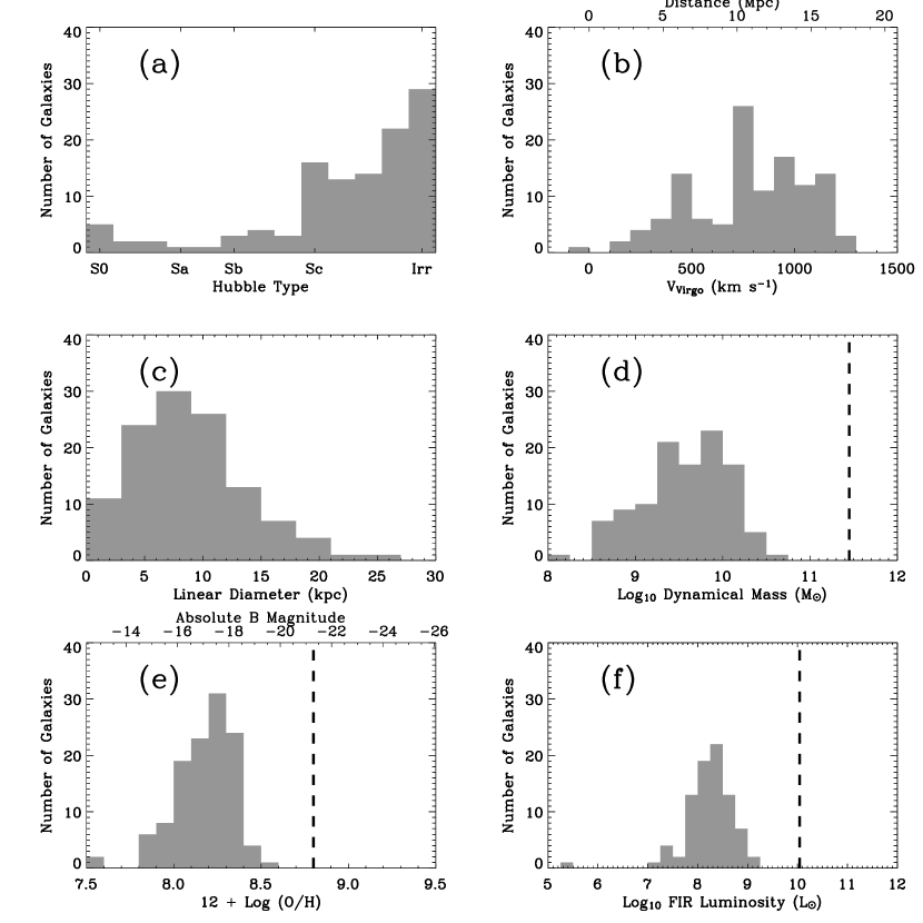
Figure 1.— A summary of some of the important properties of the galaxies in our survey: (a) the Hubble Type; (b) the recessional velocity, corrected for Virgocentric flow (equivalently distance, shown for $H_{0}=72$ km s^-1 Mpc^-1); (c) the linear diameter in kpc, using the distances from (b) and $d_{25}$; (d) the log of the dynamical mass, $M_{dyn}=v_{rot}^{2}R/G$ (in solar masses); (e) the metallicity, derived from the absolute blue magnitude (shown along the top axis) using the relation of Richer & McCall (1995); and (f) the FIR luminosity (Equation 2). Dashed lines show approximate values for the Milky Way.

2.2. ARO 12m Observations

We observed our sample with the Arizona Radio Observatory (ARO) 12m telescope at Kitt Peak. This telescope has a $55\arcsec$ half-power beam-width at 115.27 GHz. We pointed toward the optical center of our galaxies, obtained from the NASA/IPAC Extragalactic Database (NED). The data were acquired over the course of three observing runs (2001 February 1-7, 2002 January 21-25, and 2002 May 8-16) and several nights of remote observing (2001 November 27-30, 2001 December 3, 2002 May 30-June 1). Whenever possible, we observed both polarizations with the 1 MHz and 2 MHz filter banks in parallel mode, providing redundant data on each polarization. For several runs this was not an option due to hardware difficulties, and we used only one set of filter banks. We observed each source for a minimum of one hour, divided into six-minute integrations (scans). We allocated more time to sources that showed some indication of emission after the first hour, sources observed during poor weather, and those observed with only one polarization. The observing mode was usually position switching, with an offset of 2-3^′ in azimuth. In no case did we see evidence of significant emission in the reference position close to the source velocity, except for Galactic emission. Every six hours, after sunset, and sunrise, a planet or other strong continuum source was observed to optimize the pointing and focus of the telescope. The median system temperature taken over all runs was 345 K.

We reduced the spectrum for each six-minute scan in the following manner. We removed noise spikes and bad channels by flagging all channels with absolute values above the $5\sigma$ level (none of our sources were this bright in a single scan). Several channels were known to be bad a priori and we flagged these as well. We then subtracted a linear baseline from the spectrum and binned it to our final resolution of $10$ km s^-1. Finally, we averaged both polarizations and all scans to produce the final spectrum for each source. In very few ($8$) cases this procedure was not sufficient to produce a useful final spectrum, and scans with very poor baselines were either discarded or fit with a higher order polynomial.

2.3. Detection Algorithm and Integrated CO Intensity

We classified each galaxy as “detected,” “marginally detected,” or “not detected” based on the region of the spectrum containing the most statistically significant emission. We selected this region by applying the following simple algorithm to each of the final spectra. Each channel (10 km s^-1 velocity bin) within half of the H I linewidth, $W_{20}$, of the systemic velocity was used as the center of a series of spectral windows ranging from 30 to 190 km s^-1 in width (in 20 km s^-1 increments). For each of these spectral windows, we calculated the signal–to–noise ratio of the integrated intensity as

$$SNR=\frac{1}{\sqrt{N}\mbox{ }RMS}\sum_{i=1}^{N}I_{i},$$ (1)

where $I_{i}$ is the brightness temperature (intensity) in the $i$th channel within the window, $N$ is the number of spectral channels in the window, and $RMS$ is the root mean square intensity of the spectrum per channel measured in the (assumed) signal-free areas outside $\pm 100$ km s^-1 of the systemic velocity. For each spectrum, we calculated $SNR$ for all of the spectral windows that met the above criteria. With 9 spectral windows (widths of 3, 5, 7, … 17, and 19 channels) centered on each channel within $W_{20}/2$ (typically $\sim 70$ km s^-1) of the systemic velocity, we examined $\sim 135$ spectral windows per spectrum. Of these 135 values, we selected the one with the maximum signal-to-noise ratio. We refer to the SNR of this spectral window as the $SNR_{Max}$ of the spectrum.

We used a Monte Carlo technique to estimate the false positive rate of this algorithm — i.e., the probability of randomly generating a $SNR_{Max}$ higher than a given value from spectra containing only Gaussian noise. We generated a large number of artificial spectra filled with normally distributed values and containing the same number of velocity channels as our real spectra. We found that our algorithm extracted $SNR_{Max}$ values of $4.3$ or higher from these artificial spectra $<0.5\%$ of the time, indicating $\sim 99.5\%$ confidence that $SNR_{Max}\geq 4.3$ corresponds to real emission. Based on our Monte Carlo results, we classified all spectra for which we found a $SNR_{Max}$ of $4.3$ or higher as “detections.” Further, we found that our algorithm extracted a $SNR_{Max}$ of $3.0$ or higher from the artificial spectra 5% of the time. We labeled spectra with a $SNR_{Max}$ higher than $3.0$ but less than $4.3$ “marginal detections.” These thresholds, $3.0$ and $4.3$, are dependent on the number of independent channels in a spectrum and are therefore specific to our data. Given our sample of $121$ galaxies, we expect $<1$ false detection and $\sim 6$ false marginal detections. In total, we find $28$ detections (none of which we expect are false) and $16$ marginal detections ($\sim 6$ of which we expect are false). Note that we omit the marginal detections from the analysis presented in §3 and 4. However, we consider the majority of these galaxies likely to be detected in CO by future studies.

We also estimated our false negative rate — i.e., the probability that our algorithm will fail to identify a spectrum known to contain signal as a detection. We added signal with the median characteristics of our typical detections ($\sigma_{v}=50$ km s^-1, $I_{CO}=1.5$ K km s^-1) to an average noise spectrum ($RMS=0.008$ K in a 10 km s^-1 channel). Our algorithm recovered this signal as a detection $\sim 70\%$ of the time, as a marginal detection $\sim 25\%$ of the time, and not at all $\lesssim 5\%$ of the time. Under the simplifying assumption that detected galaxies represent a uniform population, our recovery rate and our $28$ detections imply a total population of $28\times\frac{1}{0.7}\sim 40$ “detectable” galaxies in our sample.

We calculated the integrated intensity of each galaxy in the following manner. For detections and marginal detections we considered the spectral window that produced the maximum signal-to-noise value. When this region was bordered by channels containing emission, we extended the window to include all contiguous channels with positive intensities. The integrated intensity of the galaxy in CO was taken to be the sum over this spectral window, and the quoted error is the statistical uncertainty over the same region. For non-detections, we measured the statistical uncertainty in the integrated intensity over a 120 km s^-1 window (the H I velocity width of a typical nondetection) centered on the radio LSR velocity of the galaxy.

Table 1 summarizes the survey results. Column (1) lists the name of the galaxy; columns (2) and (3) give the center position from NED; column (4) gives the LSR velocity of the galaxy (usually derived from the H I); column (5) lists the extinction-corrected absolute $B$ magnitude of the galaxy, derived as described below; column (6) contains the $\log_{10}$ of the FIR luminosity of the galaxy (for galaxies that lack either 60 $\mu$m or 100 $\mu$m emission, we do not report $L_{FIR}$); column (7) gives the 1.4 GHz flux associated with the central CO pointing; column (8) lists the inclination-corrected rotation velocity of the galaxy; column (9) gives the integrated intensity corrected for the main beam efficiency ($I_{CO}=\int T_{mb}dv$) derived from the CO spectrum, along with $1\sigma$ error bars (for detected galaxies), or a $3\sigma$ upper limit (for nondetections); finally, column (10) indicates whether we detected CO in that galaxy — “Y” for yes, “N” for no, and “M” indicates a marginal detection. Figure 2 shows the spectra of detections and marginal detections, with the selected spectral window shaded. The optical- and radio-derived systemic velocities are shown as vertical lines and the horizontal lines show the RMS noise derived from the signal-free regions of the spectrum. Beneath the spectrum the H I velocity width, $W_{20}$, is indicated by a dark bar. For the convenience of the reader, we note the following conversion factors: at 115 GHz with a $55^{\prime\prime}$ (half power) beam, 1 K km s^-1 corresponds to a flux of 32.9 Jy km s^-1. Assuming a Galactic CO-to-H₂ conversion factor ($2\times 10^{20}$ cm^-2 (K km s^-1)^-1, e.g. Strong & Mattox, 1996), this flux is equivalent to a molecular surface density of 4.4 $\cos i$ M_⊙ pc^-2 (including helium), where $i$ is the inclination of the galaxy in question. We shall consider variations in the conversion factor in §4.

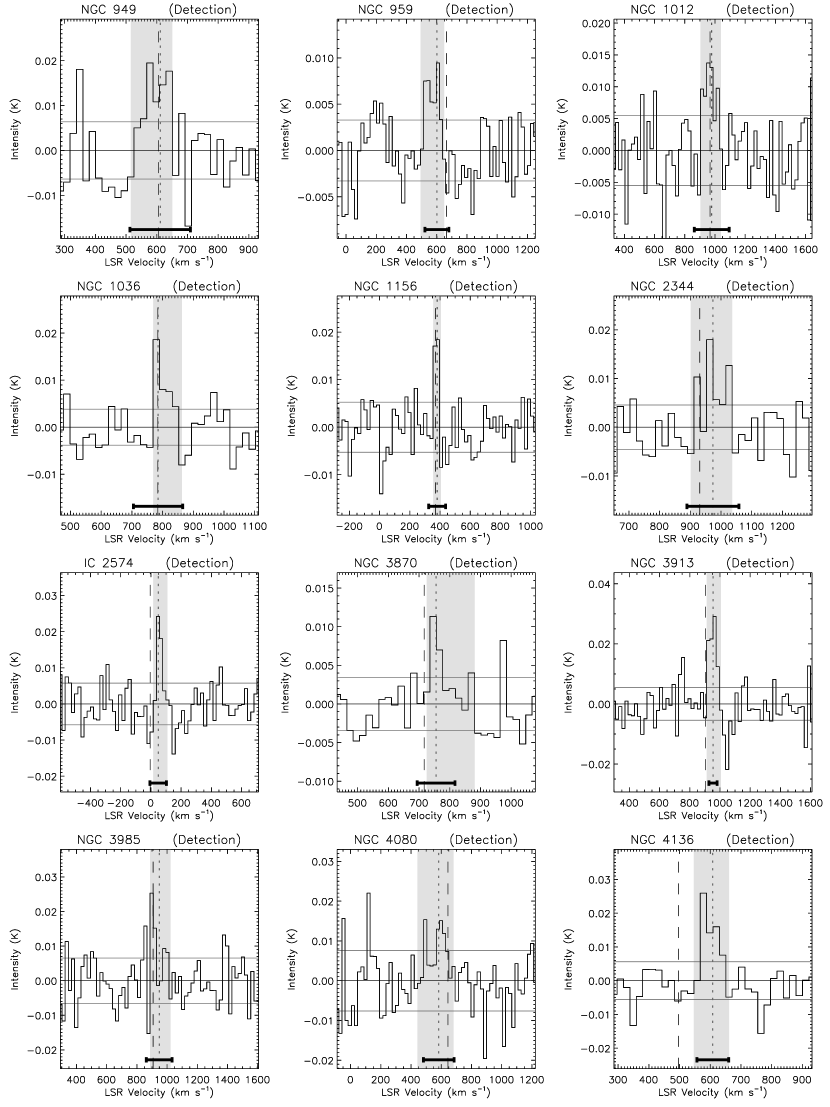
Figure 2.— Spectra of detected galaxies from the survey. The horizontal lines indicate the RMS noise calculated from the signal-free region of spectrum and the vertical lines show the position of the optical (dashed) and radio (dotted) systemic velocities. The shaded region is identified by our algorithm as emission and the black bar shows the H I linewidth, $W_{20}$. We expect $\lesssim 1$ false positive among the 28 detections and $\sim 5$ false positives among the 16 marginal detections (see §2).

Figure 2.— Spectra of detected galaxies from the survey. The horizontal lines indicate the RMS noise calculated from the signal-free region of spectrum, and the vertical lines show the position of the optical (dashed) and radio (dotted) systemic velocities. The shaded region is identified by our algorithm as emission and the black bar shows the H I linewidth, $W_{20}$. We expect $\lesssim 1$ false positive among the 28 detections and $\sim 5$ false positives among the 16 marginal detections (see §2). (continued)

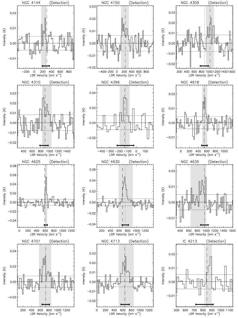
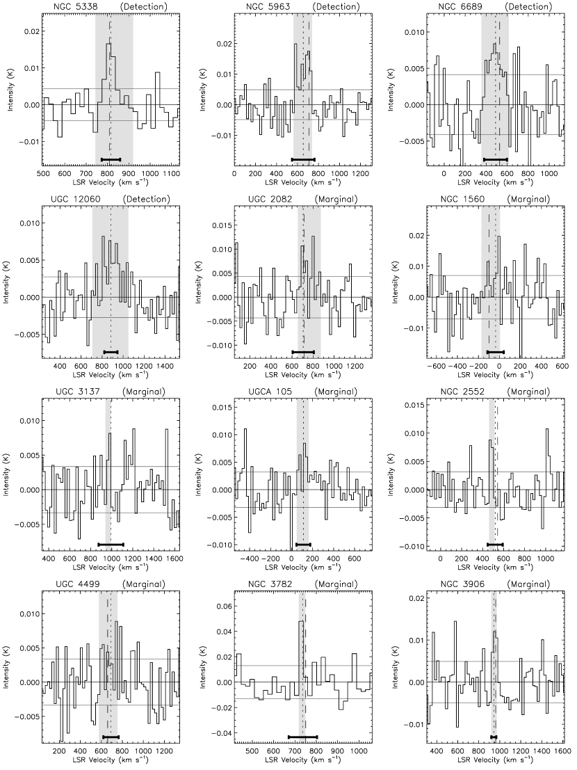
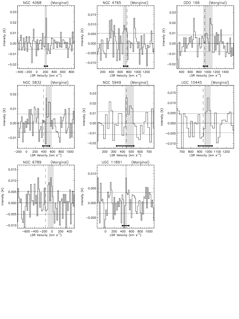
Figure 2.— Spectra of detected galaxies from the survey. The horizontal lines indicate the RMS noise calculated from the signal-free region of spectrum, and the vertical lines show the position of the optical (dashed) and radio (dotted) systemic velocities. The shaded region is identified by our algorithm as emission and the black bar shows the H I linewidth, $W_{20}$. We expect $\lesssim 1$ false positive among the 28 detections and $\sim 5$ false positives among the 16 marginal detections (see §2). (continued)

Figure 2.— Spectra of detected galaxies from the survey, followed by those of marginally detected galaxies. The horizontal lines indicate the RMS noise calculated from the signal-free region of spectrum and the vertical lines show the position of the optical (dashed) and radio (dotted) systemic velocities. The shaded region is identified by our algorithm as emission and the black bar shows the H I linewidth, $W_{20}$. We expect $\lesssim 1$ false positive among the 28 detections and $\sim 5$ false positives among the 16 marginal detections (see §2). (continued)

Figure 2.— Spectra of marginally detected galaxies from the survey. The horizontal lines indicate the RMS noise calculated from the signal-free region of spectrum and the vertical lines show the position of the optical (dashed) and radio (dotted) systemic velocities. The shaded region is identified by our algorithm as emission and the black bar shows the H I linewidth, $W_{20}$. We expect $\lesssim 1$ false positive among the 28 detections and $\sim 5$ false positives among the 16 marginal detections (see §2). (concluded)

2.4. Supplementary Data

To create a dataset that could be used to relate CO to other galaxy properties, we supplemented our survey with data from the literature. The CO data came from four sources: the observations and compilation of Taylor et al. (1998) (using the ARO 12m telescope), the FCRAO extragalactic CO survey (Young et al., 1995, using the FCRAO 14m telescope), the survey of late-type spirals by Böker, Lisenfeld, & Schinnerer (2003) (using the IRAM 30m telescope), and the survey of Elfhag et al. (1996) (using the SEST 15m telescope and the Onsala 20m telescope). We refer to this set of additional CO observations as the “supplemental sample.” Note that the supplemental sample, in particular the FCRAO survey but also the other surveys, contains a number of galaxies that do not meet our definition of dwarf galaxy (i.e., for which $v_{rot}>100$ km s^-1). These galaxies make up the sample of large galaxies used for comparison in §3 and §4. We pared the literature sample slightly, removing galaxies with Hubble types earlier than S0 and galaxies with inferred molecular masses greater than their dynamical masses. We consider either the molecular mass or the supplementary galaxy properties of such galaxies unreliable.

We obtained systemic and rotational velocities, optical magnitudes, 21-cm fluxes, inclinations, diameters, and Hubble types from the HyperLeda catalog. To these data, we added 1.4 GHz radio continuum measurements (RC), far infrared (FIR) fluxes, and $K$-band magnitudes from other sources. The RC measurements are measured from the NRAO VLA Sky Survey (NVSS) images (Condon et al., 1998), which have a resolution of $45^{\prime\prime}$ (well matched to the $55^{\prime\prime}$ 12m beam) and a sensitivity of $0.45$ mJy beam^-1. For each galaxy we calculated the RC flux integrated over the entire disk of the galaxy, which is used as a global property in §3. We also calculated the RC flux associated with the CO observation from the NVSS convolved to the resolution of that CO observation (when possible) for use in §4.

We computed the FIR flux (de Vaucouleurs et al., 1991),

$$F_{FIR}=1.26\left[2.58f_{\nu}(60)+f_{\nu}(100)\right]\times 10^{-14}\mbox{ W m}^{-2}\mbox{,}$$ (2)

using IRAS 60 and 100 $\mu$m flux densities (in Janskys) from the IRAS Faint Source Catalog (Moshir et al., 1990). $F_{FIR}$ approximates the flux in a bandpass with uniform response 80 $\mu$m wide centered at 82.5 $\mu$m. Since thermal emission from a galaxy usually peaks between 50 and 100 $\mu$m, $F_{FIR}$ is a good indicator of its total infrared flux (usually about 50%, see Bell, 2003).

The $B$-band measurements used in this paper begin as apparent, uncorrected $B$ magnitudes from the HyperLeda catalog. We correct for internal extinction following Sakai et al. (2000), and for Galactic extinction using Schlegel, Finkbeiner, & Davis (1998). We use the Virgocentric-flow corrected Hubble flow distance with $H_{0}=72$ km s^-1Mpc^-1 (Freedman et al., 2001). One galaxy in our sample, NGC 4396, has a negative distance using this method and we assigned it a distance of 20 Mpc (under the assumption that it is a member of Virgo Cluster).

We took $K$-band measurements from the 2MASS Extended Source Catalog (XSC) (Jarrett et al., 2000). We used the magnitudes obtained by extrapolating the surface brightness profile to the extrapolated K-band radius of the galaxy ($K_{ext}$ in the 2MASS XSC) because they better recover the extended flux of low surface brightness objects. In several cases the extrapolated K-band radius of the galaxy was smaller than $d_{25}/2$, which prompted us to discard the $K$-band magnitude for that galaxy as unreliable.

3. CO Emission and Galaxy Properties

In this section we examine the relationship between CO emission and other galaxy properties. We find that the strongest correlations are between the CO and the FIR, RC, $K$-band, and $B$-band luminosities. The correlation between CO, FIR, and RC presumably results from the well established association between molecular gas and star formation, but the strong correlation between CO and stellar light is somewhat surprising. It suggests that dwarf galaxies are small versions of large galaxies and that differences in the CO content among galaxies are primarily a result of scaling — a galaxy’s mass seems to be the main factor in setting its molecular gas content. We argue below that this strong correlation between molecular gas content and stellar luminosity arises from the crucial role played by the gravity of the stars in setting the midplane gas pressure and thus the local density of atomic gas — which governs the rate of H₂ formation.

3.1. Molecular Gas in Dwarf Galaxies with Detected CO Emission

We estimate the strength of the relationship between CO content and other galaxy properties using the rank correlation coefficient. The magnitude of the rank correlation coefficient gives a robust, unbiased measure of how strongly two variables are correlated but no indication of the specifics of that relationship beyond the sense (obtained from the sign). It is calculated in a manner analogous to the linear correlation coefficient, but it uses the rank of a data point within the sorted data in place of the actual value of the data point (for more details see Press et al., 1992). The rank correlation coefficient can therefore be used to distinguish whether an association exists between two galaxy properties, but contains no information on the physics of that association. To estimate the uncertainties in the coefficients we use bootstrapping methods. We create an uncorrelated dataset out of our data by randomly pairing $X$ and $Y$ data values, and then we calculate the $1\sigma$ deviation of the rank correlation coefficient around zero from many repetitions of the experiment.

Throughout this discussion we refer to the molecular mass, $M_{Mol}$, rather than the observable $L_{CO}$, as the molecular mass is the physical quantity of interest. We calculate $M_{Mol}$ by applying a Galactic CO-to-H₂ conversion factor ($X_{CO}=2\times 10^{20}$ cm^-2 (K km s^-1)^-1; Strong & Mattox, 1996) to the CO luminosity. To accurately account for the mass associated with molecular gas, we apply an additional factor of 1.36 to include the effect of helium (see the discussion in §4 for more details). Note that even if $X_{CO}$ varies from galaxy to galaxy (see §4.3 for more discussion of this issue), our results will still hold for the relationship between $L_{CO}$ and other galaxy properties.

In some cases drawn from the literature, there are observations of several fields in one galaxy. In these cases, we sum all of the emission from the galaxy to derive $M_{Mol}$. We removed galaxies with angular sizes greater than $5\arcmin$ but without observations of multiple fields from the analysis because we considered the CO in the central $1\arcmin$ an unreliable predictor of the total $L_{CO}$. Although $M_{Mol}$ is strictly a lower limit (because our observations cover only the central few kpc of each galaxy), it is likely that in dwarf galaxies the central $\sim 3$ kpc (diameter) encompassed by our survey beam contains most of the CO emission. The detections taken from the literature are, on average, farther away and therefore do an even better job of including most of the emission.

3.1.1 Molecular Gas Content and Global Properties

What properties of a galaxy are most important in setting its CO content? Are the same properties relevant in both dwarfs and large spirals? How much of the difference in the molecular gas content between dwarfs and large spirals is a result of simple scaling with galaxy size or mass? In Table 2 we present the answers to some of these questions by showing rank correlation coefficients between CO content — both normalized and total — and other galaxy properties. The values shown make use of all galaxies in our sample — large spirals and dwarfs. By including both types of galaxies we significantly extend the dynamic range over which we look for variation (e.g., see Figure 7). Typical $1\sigma$ uncertainties in the rank correlation coefficients are $0.07$ and only values with greater than $3\sigma$ significance are shown in the table; other entries are left blank.

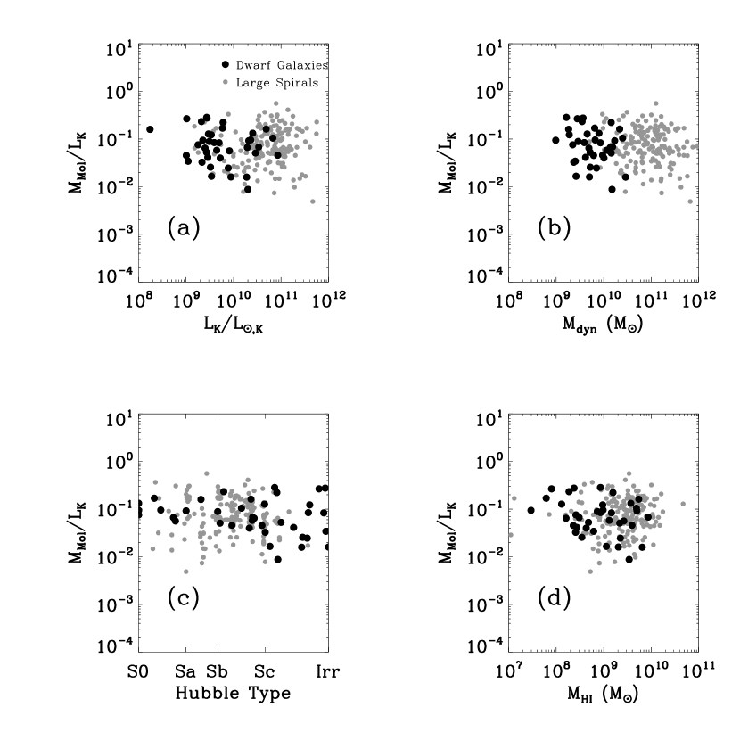
Figure 7.— Molecular gas mass per unit $K$-band luminosity is remarkably constant as a function of galaxy mass and morphology. Each panel shows $M_{Mol}/L_{K}$ as a function of a different galaxy property. Panel (a) shows $K$-band luminosity, a tracer of stellar mass; panel (b) show dynamical mass; panel (c) shows galaxy morphology; and panel (d) shows atomic gas mass. In each case dwarfs (black dots) and large galaxies (gray dots) show the same median $M_{Mol}/L_{K}\approx 0.075M_{\odot}/L_{\odot,K}$ and little or no variation with the independent variable. Dwarfs are defined as galaxies with H I inclination-corrected rotational velocities, $v_{rot}$, less than 100 km s^-1.

We also indicate in Table 2 whether two quantities are significantly correlated within the sample of dwarfs alone. Entries in boldface indicate that the two quantities are correlated at $3\sigma$ significance or greater in the subset of dwarf galaxies. Typical uncertainties in the rank correlation coefficients among the dwarfs are $0.16$, so that boldfaced entries have rank correlation coefficients $\gtrsim 0.5$ within the dwarf subset alone (and none exceed $0.7$). In only one case, the correlation between $M_{HI}$ and $M_{Mol}/M_{HI}$, do two quantities correlate significantly within the dwarfs but not in the larger sample.

The second column in Table 2 shows that $M_{Mol}$ is correlated with a number of other galaxy properties at a very high significance — including Hubble type, dynamical mass, $K$-band luminosity, $B$-band luminosity, FIR luminosity, RC luminosity, linear diameter, and atomic hydrogen content. Figure 8 illustrates several of these correlations graphically, with dwarf galaxies plotted as black circles and large galaxies as gray circles. All of the correlations are in the same sense, namely that more massive galaxies with earlier Hubble types and redder colors have more molecular gas. In order to investigate the question of whether dwarf galaxies are merely smaller version of large spirals, we must look past scaling effects and examine how the normalized CO content of a galaxy changes with its other properties.

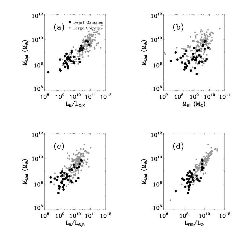
Figure 8.— Molecular gas mass as a function of several galaxy properties: (a) $K$-band luminosity, (b) atomic gas mass, (c) $B$-band luminosity, and (d) FIR luminosity. Dwarfs are defined as galaxies with inclination-corrected rotational velocities, $v_{rot}$, less than 100 km s^-1.

3.1.2 Normalized Molecular Gas Correlations

Columns (3) through (5) of Table 2 show that many of the strong correlations between CO content and other galaxy properties are removed when the CO content is normalized by the stellar or dynamical mass of the galaxy. In particular the quantity $M_{Mol}/L_{K}$ (column 3) shows very little systematic variation with other galaxy properties (also see Figure 7). The median $M_{Mol}$/$L_{K}$ is $\approx 0.075\pm 0.005M_{\odot}/L_{\odot,K}$ for large spirals and $\approx 0.065\pm 0.008M_{\odot}/L_{\odot,K}$ for dwarf galaxies, identical within the uncertainties — Figure 7 shows this constancy. We find that similar results are achieved when normalizing $M_{Mol}$ by the dynamical mass, $M_{dyn}$ (see column 4 of Table 2) — $M_{Mol}/M_{dyn}\approx 0.040\pm 0.003$ for large spirals and $0.037\pm 0.007$ for dwarfs, again virtually identical. The difference in $M_{Mol}$/$L_{B}$, which is $\approx 0.16\pm 0.01M_{\odot}/L_{\odot,B}$ for large spirals and $\approx 0.13\pm 0.02M_{\odot}/L_{\odot,B}$ for dwarf galaxies, is also not significant. The weak, but significant, correlations between $M_{Mol}$/$L_{B}$ and $L_{K}$, $B-K$, $M_{HI}/L_{K}$, and $M_{dyn}/L_{K}$ may reflect the fact that large galaxies tend to have redder stellar populations than small galaxies. Also note that, although we apply an extinction correction to the $B$-band luminosity that varies with galaxy size (Sakai et al., 2000), extinction effects may still be important.

These same results hold for a sample consisting of only dwarf galaxies. $M_{Mol}$ in dwarfs correlates strongly with $L_{K}$, $L_{B}$, and linear diameter. As in the larger sample, the $3\sigma$ correlations found within the dwarf galaxies disappear if the CO content is normalized by galaxy (stellar) mass. Thus we find little evidence for systematic variations in the quantities $M_{Mol}/L_{K}$, $M_{Mol}/M_{dyn}$, and $M_{Mol}/L_{B}$ with galaxy mass. This suggests that dwarf galaxies are indeed “small versions” of large galaxies and that differences in the CO content among galaxies are primarily a result of scaling — a galaxy’s mass seems to be the main factor in setting its molecular gas content and (stellar) mass alone can explain most of the correlations seen in column (2) of Table 2.

The ratio of molecular to atomic gas, on the other hand, is a strong function of other galaxy properties. Table 2 and Figure 9 show the well-established trend of decreasing $M_{Mol}/M_{HI}$ with later Hubble type and decreasing galaxy mass (see Young & Scoville, 1991, and references therein). The dwarf galaxies in our sample tend to be low mass systems with late Hubble types and therefore have lower $M_{Mol}/M_{HI}$ than large spirals — $0.3\pm 0.05$ compared to $1.5\pm 0.1$. Although dwarf galaxies tend to have roughly the same amount of molecular gas per unit stellar mass, their ISMs are dominated by large reservoirs of atomic gas and the molecular gas makes up only a small fraction of the total gas mass.

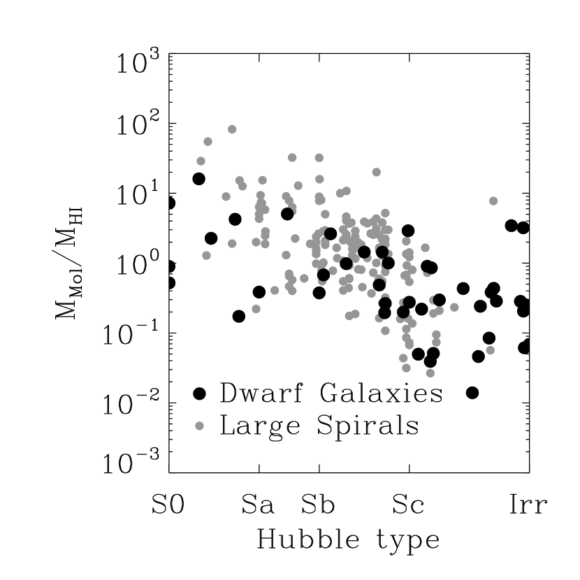
Figure 9.— The ratio of molecular to atomic gas as a function of Hubble type. Later type galaxies, including most of the dwarfs in our sample, have less molecular gas per unit atomic gas than galaxies with earlier Hubble types. Dwarfs are defined as galaxies with H I inclination-corrected rotational velocities, $v_{rot}$, less than 100 km s^-1. The two irregular galaxies with very large molecular fractions in Figure 9 are NGC 4630 and NGC 4080. It seems quite possible that we have overestimated the CO flux of NGC 4080 (see Figure 2), but NGC 4630 clearly has much more CO emission than one would expect based on its other properties.

CO and FIR emission trace the amount of molecular gas and ongoing star formation, respectively. Therefore the quantity $\tau_{Dep}=M_{Mol}/L_{FIR}$ is a proxy for the depletion time, the time it will take for a galaxy to consume its reservoir of molecular gas at its present rate of star formation. Columns (7) and (8) of Table 2 and Figure 10 show that $\tau_{Dep}$ varies systematically with galaxy mass. Figure 10 shows that there is an anticorrelation between galaxy mass and the depletion time within our sample of dwarfs. Figure 10 also shows that there is a positive correlation between mass and depletion time for large galaxies. This latter result has been noted previously in a careful study of face-on undisturbed galaxies by Young (1999). She found that galaxies with diameters of $\sim 15$ kpc had the longest depletion times in her sample (which did not include dwarfs), and that the depletion times in larger galaxies increased with increasing diameter.

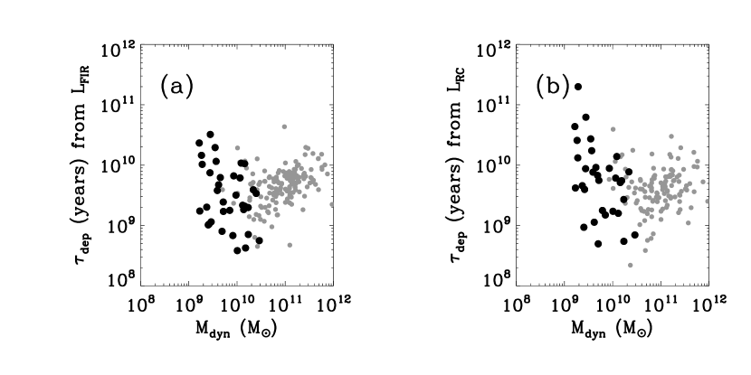
Figure 10.— Molecular gas depletion time decreases with galaxy mass among dwarf galaxies (black dots) and then increases with galaxy mass among large galaxies (gray dots). The two panels show the same effect using different star formation tracers. Panel (a) shows $\tau_{Dep}$ calculated using the high mass star formation rate inferred from $L_{FIR}$ and panel (b) shows $\tau_{Dep}$ calculated from the high mass star formation rate derived from the radio continuum luminosity. Galaxies with masses $M_{dyn}\sim 10^{10}M_{\odot}$ and appear able to convert their molecular gas into stars most efficiently. Dwarfs are defined as galaxies with H I inclination-corrected rotational velocities, $v_{rot}$, less than 100 km s^-1.

Here we find that below masses of $\sim 10^{10}M_{\odot}$ and diameters of $\sim 10$ kpc the depletion time tends to rise with decreasing galaxy mass/size, so that galaxies with masses of $\sim 10^{10}M_{\odot}$ seem to be maximally efficient at turning molecular gas into stars. Later in this paper, we find that molecular gas depletion time decreases with increasing surface density of molecular gas. That is, the higher the surface density of molecular gas the more quickly it will be consumed by star formation. We suggest that this effect drives the behavior in the dwarfs shown Figure 10. Galaxies of $\sim 10^{10}M_{\odot}$ have higher average surface densities of molecular gas than do smaller galaxies and therefore they display slightly lower depletion times (i.e. higher star formation efficiencies).

Based on our examination of the normalized molecular gas content we find that the amount of molecular gas per unit stellar mass or dynamical mass is roughly constant across more than two orders of magnitude in galaxy mass. Over this same range, the molecular gas depletion time does vary, but not particularly strongly. On the other hand, smaller galaxies tend to be much richer in atomic gas than large galaxies and therefore have much smaller fractions of their total gas mass in molecular form than large galaxies. These results suggest that the dwarf galaxies in our sample do look very much like scaled down versions of large galaxies, with the major difference being the presence of a reservoir of atomic gas in smaller systems — gas that is apparently irrelevant to star formation. Table 3 shows the power law exponents derived from fits of $M_{Mol}$ to several galaxy mass and star formation tracers. That the slopes are all very close to unity reinforces the conclusion that variations in $M_{Mol}$ may be just the result of mass scaling.

3.1.3 The Molecular ISM of Dwarf Galaxies

The strongest correlations in our sample (both considering the dwarfs alone and the combined set of dwarfs and large spirals) are between the molecular gas content, $M_{Mol}$, the $K$-band luminosity, $L_{K}$, the $B$-band luminosity, $L_{B}$, and the FIR luminosity, $L_{FIR}$, of galaxies. The correlation between $M_{Mol}$ and $L_{FIR}$ is well known in large spiral galaxies (e.g., Young & Scoville, 1991): $L_{FIR}$ is dust-reprocessed light from young stars, which have recently formed out of the molecular gas. The relationship between $M_{Mol}$ and the $K$-band luminosity (dominated by K-giants and other old stars — a proxy for the total stellar mass of a galaxy), is more puzzling. A power law fit of $M_{Mol}$ to $L_{K}$ predicts the CO content of a dwarf with less scatter ($\sim 0.4$ dex) than a similar fit to $L_{B}$ ($\sim 0.5$ dex) or $M_{dyn}$ ($\sim 0.7$ dex). Further, the slope of the best fit power law is nearly unity $1.3\pm 0.2$ and normalization by $L_{K}$ removes almost all correlation between $M_{Mol}$ and other galaxy properties — unlike normalization by $L_{B}$, which leaves weak but significant correlation with $L_{K}$ (see Tables 2 and 3).

Why should the correlation between molecular gas content and the mass of old disk stars be as strong as that between molecular gas content and the light of the young stars that form directly out of that gas? Further, why should the correlation between molecular gas content and the old disk stars be so much stronger than that between the molecular gas mass and the mass of the atomic gas from which it forms? We suggest that this correlation arises because the hydrostatic pressure in the galactic disk regulates the rate at which H₂ forms out of H I, and that the stellar surface density drives the midplane hydrostatic pressure.

Recently, Wong & Blitz (2002) and Blitz & Rosolowsky (2004) suggested that the hydrostatic gas pressure plays a dominant role in setting the ratio of atomic to molecular gas in disk galaxies. They show that the midplane hydrostatic gas pressure, $P_{h}$, in a stellar-dominated galactic disk can be written:

$$P_{h}\propto\sqrt{\Sigma_{*}}\,\Sigma_{g}\,\frac{\sigma_{v}}{\sqrt{h_{*}}},$$ (3)

where $\Sigma_{g}$ is the surface density of gas in the disk, $\sigma_{v}$ is the gas velocity dispersion, $\Sigma_{*}$ is the surface density of the stars, and $h_{*}$ is the stellar scale height. There is good evidence that $\sigma_{v}$ and $h_{*}$ are nearly constant within and among disk galaxies and that radial variations in the surface density of atomic gas, $\Sigma_{HI}$, are small compared to radial variations in $\Sigma_{*}$ (see references in Blitz & Rosolowsky, 2004; Shostak & van der Kruit, 1984; Kregel, van der Kruit, & de Grijs, 2002). Therefore, in the atomic-dominated regions of large disk galaxies, the portions of these galaxies most similar to the dwarf galaxies in this paper, the dominant variable setting the midplane gas pressure is $\Sigma_{*}$. Indeed, in a sample of spiral galaxies, Blitz & Rosolowsky (2004) found that the transition from a molecule-dominated ISM to an atomic-dominated ISM comes at a nearly constant stellar surface density, $120$ M_⊙ pc^-2. If $P_{h}$ is set largely by $\Sigma_{*}$ and the molecular gas abundance is determined by $P_{h}$, this would explain the good correlation between $M_{Mol}$ and $L_{K}$ within our sample.

Why should $P_{h}$ control the conversion of H I into H₂? The gas pressure is given by $P_{h}=\rho_{g}\sigma_{v}^{2}$, so in a medium with constant velocity dispersion, $\sigma_{v}$, $P_{h}$ is directly proportional to the local gas density, $\rho_{g}$. The local gas density sets the rate of H₂ formation, with formation $\propto\rho_{g}^{2}$ (Hollenbach, Werner, & Salpeter, 1971). In practice, the equilibrium abundance of H₂ may depend more weakly on the local gas density, because the strength of the dissociating radiation field is likely to be higher in regions of high gas density.

Indeed, several observations suggest that lower $K$-band luminosities of dwarf galaxies should correspond to lower average gas densities. The average H I surface density in the centers of dwarf galaxies correlates well with their central stellar surface brightness (Swaters et al., 2002), and the central stellar surface brightness increases with increasing luminosity (see e.g. Blanton et al., 2003). Therefore we expect higher gas surface densities, $\Sigma_{g}$, in higher luminosity systems. Furthermore, shallower stellar potentials yield larger gas scale heights, $h_{g}$, which translate into a further decrease in the mean gas density $\rho_{g}\sim\Sigma_{g}/h_{g}$. Despite their large reservoirs of atomic gas, smaller galaxies with less developed disks and shallower stellar potential wells lack the gas densities necessary to efficiently convert H I into H₂.

Thus, we suggest that the link between the $K$-band luminosity and the molecular gas mass $M_{Mol}$ is the hydrostatic gas pressure, or equivalently the local gas density. Because higher $K$-band luminosities correspond to larger stellar surface densities, higher values of $L_{K}$ lead to larger midplane pressures and correspondingly higher gas densities, making the H I$\rightarrow$H₂ conversion more efficient. This effect translates into a greater abundance of molecular gas in more luminous $K$-band galaxies, resulting in more star formation (see §4 for a discussion of the relationship between CO and star formation) and the young, massive stars thus produced will fuel the FIR luminosity of the galaxy.

While consistent with our data, this picture is not the only possible interpretation. An alternative conclusion might be that in dwarf galaxies (or actively star forming galaxies) the $K$-band light is a good tracer of the star formation rate. For instance, Regan & Vogel (1994), in a near-IR study of M 33 (a galaxy that is intermediate between our dwarfs and the large spirals) found that OB stars may affect the near-IR emission of a galaxy by as much as $50\%$. Two observations lead us to prefer the stellar potential well explanation offered above. First, the $K$-band light appears to be a better predictor of CO content than the $B$-band light, which should be even more sensitive to the population of young stars than the $K$-band light. Second, the ratio of $M_{Mol}/L_{K}$ remains constant across a range of morphologies (see Figure 7c) and stellar populations — in earlier-type galaxies the $K$-band light is certainly not dominated by young stars and $M_{Mol}/L_{K}$ seems to be constant among these systems and late-type, lower mass dwarfs. This suggests that $L_{K}$ traces an older stellar population throughout our sample.

3.2. The CO Nondetections

How does this picture mesh with the properties of our CO nondections? Here we restrict our investigation to our survey, a well defined sample including detections and nondetections. We looked for statistical differences between selected properties of galaxies classified as detections and those of nondetections. Table 4 gives median values for nondetections and detections for each property and Table 5 summarizes the significance of these differences. Figures 11 and 12 show the populations of detections and nondetections for a number of properties of interest.

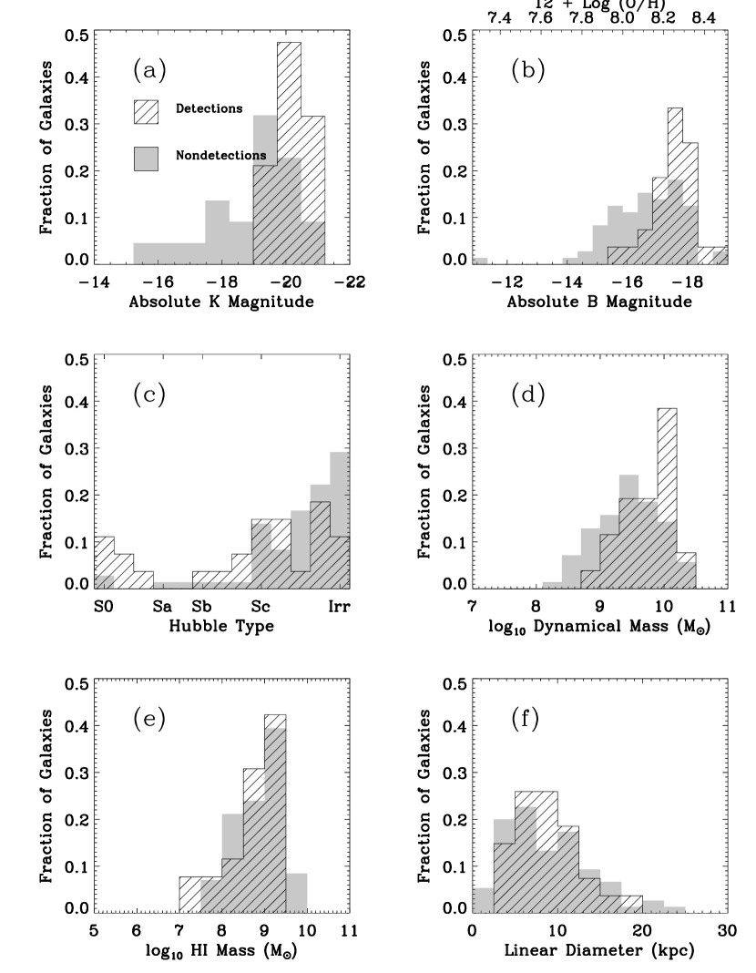
Figure 11.— Histograms showing the difference between detections (hashed) and nondetections (filled) in distributions of various parameters tracing galaxy size.

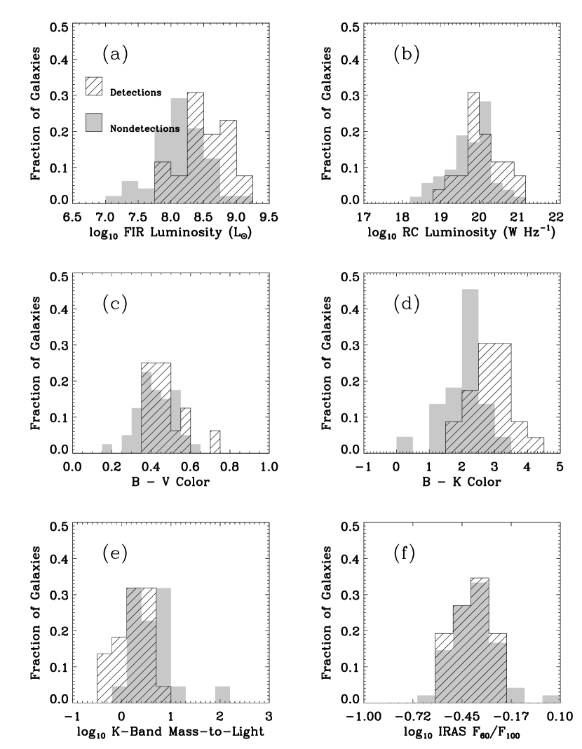
Figure 12.— Histograms showing the difference between detections (hashed) and nondetections (filled) in distributions of star formation tracers, optical and infrared colors, and mass-to-light ratios.

We calculated the significance of the differences in Table 4 in the following manner. For each property, we used two statistics to test the hypothesis that the samples of detected and nondetected galaxies were drawn from the same parent population. First, we used a two-sided Kolmogorov-Smirnov (KS) test, which considers the maximum difference between the cumulative probability distributions of the two populations. Second, we applied the Student’s $t$ test, which considers the difference between the means of the two distributions. To estimate the significance of the results we used a Monte Carlo approach, where we applied the tests to randomly selected subsamples of the observed galaxies. Significant measures of the differences between detected and nondetected galaxies are those that are unlikely to be obtained from randomly selected subsamples. The numbers listed in Table 5 are the fraction of randomly generated pairs of populations that produce a greater (more significant) difference than we observe between the detected and nondetected galaxies under the KS and Student’s $t$ test, so that very small numbers indicate very significant differences between the detections and nondetections for that property.

Table 5 shows that, not surprisingly, the distributions of most of the galaxy properties seen to be strongly correlated to CO in Table 2 also differ quite significantly between detections and nondetections — the most notable exception being the linear diameter, which fails to distinguish between detections and nondetections. The populations of absolute K magnitudes and absolute B magnitudes differ between the detections and nondetections at greater than $\sim 99\%$ significance in the sense that brighter galaxies are more likely to be CO detections. Our two tracers of global star formation rate, FIR luminosity and radio continuum luminosity, show the same trend — higher SFR increases the chances of detecting CO (although this effect is of only marginal significance for $L_{RC}$). As in Table 2, the total H I mass associated with the system seems to be a relatively poor indicator of CO content. Nondetections and detections have approximately the same amount of atomic hydrogen, so that the nondetections are, in fact, more gas rich (measured by $M_{HI}/L_{B}$) than the detections.

Thus, the picture outlined in the previous subsection appears to apply to the CO nondetections in our survey. Galaxies with low stellar masses (traced by the $K$-band and $B$-band luminosities) tend to be nondetections even though they have comparable reservoirs of atomic gas to the CO detections. We suggest that this is because the lower surface density in the stellar disks of the nondetections leads to a more diffuse, low-pressure distribution of atomic gas, one that is consequently less suitable for converting atomic gas into molecular gas.

3.2.1 Portrait of a Detection and a Nondetection

There is considerable latitude within the classification of a galaxy as a “dwarf,” so here we paint a rough picture of the types of galaxies that we detect in our survey and the types of galaxies that remain beyond our detection limits.

Our detections tend to be dwarf spirals similar in luminosity and mass to the LMC, though typically richer in CO and forming stars somewhat less vigorously. Their median dynamical mass and B-magnitudes ($M_{dyn}=8\times 10^{9}$ M_⊙ and $M_{B}=-17.6$) are comparable to those of the LMC (which has $M_{dyn}\approx 8\times 10^{9}$ M_⊙ and $M_{B}\approx-17.8$; Kim et al., 1998). Most of our detections an order of magnitude greater CO luminosity than the LMC ($\approx 2\times 10^{6}$ K km s^-1 pc²; Mizuno et al., 2001a) within our $\sim 3$ kpc beam. Although most of the CO emission in the LMC is concentrated within a $\sim 3$ kpc area, this area is not at the optical center of the galaxy. Therefore this luminosity is actually an upper limit to what we would expect to detect if an LMC analog were included in our sample, and about a fifth of detected galaxies show CO luminosities similar to or less than this value. Assuming a Galactic CO-to-H₂ conversion factor, the median CO mass for a detection is $8\times 10^{7}$ M_⊙, about 10% of the median H I mass. This molecular fraction is about order of magnitude lower than what is typical in large spirals. Most of our galaxies have earlier Hubble types (median Sc) than the LMC (Sm). The median FIR luminosity of a detection is $\sim 3\times 10^{8}~{}L_{\odot}$, about half that of the LMC.

The nondetections are typically less massive and less luminous than the detections and have later Hubble Types. Both their median dynamical mass and their median optical luminosity ($M_{dyn}=3\times 10^{9}$ and $M_{B}=-16.8$) are similar to that of the SMC ($M_{dyn}=2.4\times 10^{9}$ M_⊙ (Stanimirović, Staveley-Smith, & Jones, 2004) and $M_{B}=-16.6$) and the Local Group galaxy IC 10 ($M_{B}=-16.4$). The median FIR luminosity of a nondetection is $1.5\times 10^{8}~{}L_{\odot}$, which is several times higher than that of the SMC ($4.4\times 10^{7}~{}L_{\odot}$) or IC 10 ($3.6\times 10^{7}~{}L_{\odot}$ Melisse & Israel, 1994). This should not be surprising, since we required a galaxy to be detected by IRAS in order to be included in our sample. The galaxies that we do not detect, then, are dwarf irregulars with stellar masses similar to the SMC though with significantly more vigorous star formation.

Thus, the molecular gas in very primitive systems, the distant cousins to the SMC, remains tantalizingly out of reach. Mizuno et al. (2001b) found a CO luminosity of $8\times 10^{4}$ K km^-1 pc² for the SMC (though they did not survey the entire galaxy). If all of this gas were concentrated within the 12m beam, it would yield an intensity (averaged over the beam) of $\sim 1$ K km s^-1 at 1 Mpc, slightly lower than the median intensity of one of our detections ($1.5$ K km s^-1). At the distance of our nearest nondetection (2.2 Mpc), the SMC drops to $\sim 0.25$ K km s^-1, which is undetectable by our observations (the lowest intensity for which we detect CO in this sample is $0.5$ K km s^-1). At the 11 Mpc median distance to a member of our sample, this intensity drops to $\sim 0.01$ K km s^-1, far below our detection limits. The SMC, however, is too faint in the FIR to have made it into our IRAS-selected sample at such a distance.

3.2.2 FIR Color

Does the size and temperature of the dust grains affect the CO emission from a galaxy? Dust helps to shield the gas from dissociating UV radiation and is believed to provide the sites for H₂ formation. Variations in either the size distribution or temperature of the dust in a galaxy might have an important effect on the molecular gas content of that galaxy, especially since the range of temperatures at which molecular gas can form on dust grains may be quite small. Using the IRAS measurements at 12, 25, 60, and 100 $\mu$m we looked for systematic variations in the FIR colors of our galaxies that might be correlated with molecular gas content.

Galaxies detected in CO are also detected by IRAS at 12$\mu$m and 25$\mu$m at a much higher rate than CO nondetections (2 of the 74 nondetected galaxies have associated IRAS 12$\mu$m emission and only 11 are detected at 25$\mu$m; by comparison, 10 of the 28 detected galaxies show 12$\mu$m emission and 11 show 25$\mu$m emission). It is tempting to interpret this comparative lack of 12$\mu$m emission among the nondetected galaxies as arising from a preferential depletion of small grains analogous to that seen in the SMC (Sauvage, Vigroux, & Thuan, 1990). However, the upper limits associated with the 12$\mu$m emission in the CO nondetections are high enough that these galaxies could have the same $F_{12}$/$F_{100}$ ratio as the CO detections and still not appear in the 12 $\mu$m catalog. Thus a deficiency of small grains is not ruled out, but there is no strong evidence for it. In addition, CO nondetections in which 25 $\mu$m emission is seen have the same median $F_{25}$/$F_{100}$ ratio as the CO detections ($\sim 0.05$).

The $F_{60}$/$F_{100}$ ratio, an indicator of the temperature of dust in these galaxies, also shows no significant variation between detections and nondetections ($F_{60}$/$F_{100}\approx 0.40$ for nondetected galaxies and $0.41$ for detected galaxies). Further, column (2) in Table 2 shows that there is no significant correlation between FIR color and total molecular gas content. Within the combined sample of dwarfs and large spirals, $F_{60}$/$F_{100}$ does correlate with the normalized molecular gas content of a galaxy. Galaxies with higher $F_{60}$/$F_{100}$ ratio tend to have more molecular gas per unit mass/luminosity than less “infrared-blue” galaxies. Columns (7) and (8) also show that such galaxies also have shorter depletion times. This is a result of the fact that $F_{60}$/$F_{100}$ is an excellent predictor of $L_{FIR}$ for a given $L_{K}$ (or other mass indicator) — $F_{60}$/$F_{100}$ and $L_{FIR}/L_{K}$ are correlated at $\sim 10\sigma$, hardly surprising given the definition of $L_{FIR}$ (see Equation 2). Since there is not even a suggestion of these trends within the dwarf population alone, the usefulness of the far infrared color as a predictor of CO emission within dwarfs appears to be negligible. If a trend is present, the scatter among galaxies is too large for it to be useful.

3.2.3 Metallicity

It has long been thought that the abundance of heavy elements in a galaxy may be closely linked to its CO emission (Maloney & Black, 1988; Taylor et al., 1998). Here we look for such an effect in our sample. However, the number of well-determined metallicities for dwarf galaxies remains small. Fortunately, within galaxies which do have known metallicities there is a strong correlation between the $B$-band luminosity of a dwarf galaxy and its metallicity (Richer & McCall, 1995). In fact, in dwarf irregulars the $B$-band luminosity is a better predictor of metallicity than the central surface brightness (see Skillman, Côté, & Miller, 2003, and references therein). The fit,

$$12+\log\mbox{(O/H)}=(5.67\pm 0.48)+(-0.147\pm 0.029)M_{B}$$ (4)

is derived from Local Group dwarf irregulars (Richer & McCall, 1995) but also describes Sculptor Group dwarf irregulars well (Skillman, Côté, & Miller, 2003) and the slope agrees within the uncertainties with that found for dwarf galaxies using the best quality data in the 2dF Galaxy Redshift Survey (Lamareille et al., 2004). For luminosities fainter than $M_{B}=-15$ there is significant scatter, usually towards higher than predicted abundances, but only a few of our galaxies — all nondetections — are this faint.

Figure 13 shows that there is significant difference in the $B$-band derived metallicities of the detections and nondetections in our survey. Above $12+\log\mbox{(O/H)}=8.2$, 21 of the 52 galaxies in our sample are detected (a further 3 are marginally detected). Below that value only 6 of the 62 galaxies were detected (and 9 are marginally detected). This drop in detection rate is difficult to conclusively attribute to metallicity effects. Metallicity is strongly correlated with other galaxy properties — indeed, we are using B magnitude as a proxy for metallicity here — and it is not clear whether a drop in detection rates at low metallicities is caused by lower metallicities or by the effects of other parameters that are covariant with metallicity. Regardless, we do find agreement with Taylor et al. (1998) who found that detections of galaxies with metallicities of $12+\log\mbox{(O/H)}\approx 8.0$ or less are quite rare. It remains to be determined whether this is simply because such systems have less molecular mass or because they form less CO per unit molecular mass.

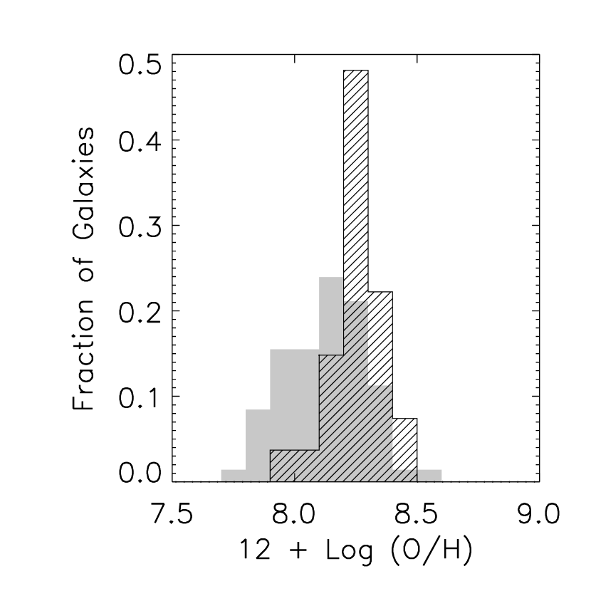
Figure 13.— Metallicities (derived from absolute $B$-band magntiudes) of dwarf galaxies in our survey. Nondetections (the solid gray histogram) have systematically lower metallicities than detections (the hashed histogram). Below $12+\log\mbox{(O/H)}\sim 8.2$ the detection rate drops from $\approx 50\%$ to $\approx 20\%$.

4. Molecular Gas and Star Formation in Dwarf Galaxies

We have already seen (in Table 2 and the previous section) that there is a strong association between molecular gas and star formation — traced by FIR and RC emission — in our sample. Here we investigate whether that association is the same in dwarf galaxies and large spiral galaxies. Specifically, we ask: do dwarf galaxies differ from large spiral galaxies in their mode of star formation, as measured by the relationship between the surface density of molecular gas, $\Sigma_{Mol}$, and the surface density of star formation, $\Sigma_{SFR}$? There is reason to think that this might be the case. Dwarfs differ from large spirals in a number of important respects: luminosity, mass, metallicity, large scale dynamical effects (such as spiral density waves and supernova-driven shocks), dust properties, UV radiation field, and possibly magnetic field strength. Each of these differences could conceivably change the properties of molecular clouds in a manner that affects the rate at which stars form out of molecular gas. Any such difference should manifest itself as a different large scale relationship between $\Sigma_{Mol}$ and $\Sigma_{SFR}$.

4.1. The CO-to-RC Relationship in Dwarfs and Large Spirals

Radio continuum offers two major advantages over other star formation tracers for the work in this section: 1) RC data are free of extinction and 2) the entire sky is available in the NVSS at $45^{\prime\prime}$ resolution (comparable to the $55^{\prime\prime}$ 12m beam). This latter advantage allows us to measure $\Sigma_{SFR}$ with the same resolution that we use to measure $\Sigma_{Mol}$ ($\sim 3$ kpc for a typical dwarf galaxy). Figure 14 shows the RC brightness (flux density, in mJy, per $45^{\prime\prime}$ beam), $B_{\nu,1.4}$, and the integrated CO intensity, $I_{CO}$ (in K km s^-1), associated with CO pointings from our survey and the supplemental sample (only galaxies with both CO and RC detected at $\geq 2\sigma$ significance are included).

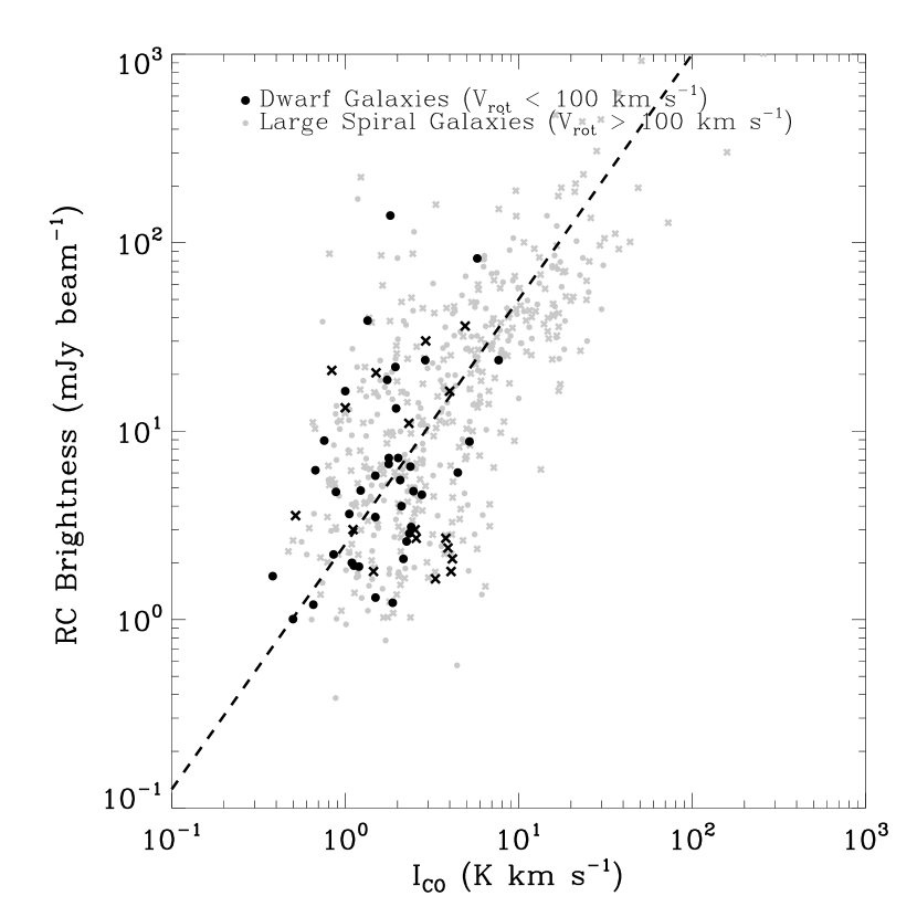
Figure 14.— The 1.4 GHz radio continuum brightness (flux density per $45^{\prime\prime}$ beam) plotted against integrated intensity for dwarf galaxies (black points) and large spiral galaxies (gray points). The dashed line shows the best fit to the two populations combined. In contrast to Figure 15, all galaxies are plotted here. Some galaxies were discarded from our analysis because of their large angular sizes or early Hubble Types (see discussion in §4). These are plotted as crosses rather than circles and not used in the fit.

Figure 14 shows that $B_{\nu,1.4}$ and $I_{CO}$ are highly correlated in both large spirals and dwarfs. This association has long been known in large spirals (Adler, Lo, & Allen, 1991; Murgia et al., 2002) and we see here that it extends seamlessly to dwarf galaxies. Indeed, we find that the power laws that best describe the two datasets independently,

$$B_{\nu,1.4}^{\mathrm{Large~{}Spirals}}~{}\left(\mathrm{mJy~{}beam}^{-1}\right)=10^{0.5\pm 0.1}~{}I_{CO}^{1.4\pm 0.2}~{}\left(\mbox{K km s}^{-1}\right)$$ (5)

and

$$B_{\nu,1.4}^{\mathrm{Dwarfs}}\left(\mathrm{mJy~{}beam}^{-1}\right)=10^{0.5\pm 0.1}~{}I_{CO}^{1.5\pm 0.2}~{}\left(\mbox{K km s}^{-1}\right)$$ (6)

agree within the uncertainties. The simplest interpretation for this agreement is that dwarfs and large spirals show the same relationship between molecular gas and star formation and that the CO and RC trace these physical quantities in the same way in all galaxies. In this context, dwarf galaxies appear to be simple low mass mass versions of large spirals.

To arrive at the relationship between $\Sigma_{Mol}$ and $\Sigma_{SFR}$, we use the following relations (based on those of Murgia et al., 2002) to convert RC surface brightness and $I_{CO}$ into the physical quantities of interest,

$$\Sigma_{SFR}\left(\frac{M_{\odot}}{\mbox{yr kpc}^{2}}\right)=8.0\times 10^{-4}$$ (7)

$$\times~{}B_{\nu,1.4}\left(\mathrm{mJy~{}beam}^{-1}\right)\,\left({\frac{\theta}{\mbox{45\arcsec}}}\right)^{-2}\cos i$$

$$\Sigma_{Mol}\left(\frac{M_{\odot}}{\mathrm{pc^{2}}}\right)=4.4~{}I_{CO}\left(\mbox{K km s}^{-1}\right)~{}\cos i\mbox{,}$$ (8)

where $\theta$ is the linear size of the CO beam (in ″) or 45″, whichever is larger. These equations assume linear relationships between $B_{\nu,1.4}$ and $\Sigma_{SFR}$ for all galaxies and a constant conversion factor of $X_{CO}=2\times 10^{20}$ cm^-2 (K km s^-1)^-1 (i.e., the Galactic value, Strong & Mattox, 1996). We will consider the effect of relaxing these assumptions in §4.3. Note that Equation 8 includes a factor of 1.36 to account for the presence of helium (hence we call it $\Sigma_{Mol}$ rather than $\Sigma_{H_{2}}$). The purpose of this convention is to account accurately for the mass of molecular clouds and its conversion to stellar mass in §4.2.

Our CO dataset is composed of observations with resolutions that range from $24\arcsec$ to $55\arcsec$. For CO pointings observed with a beam larger than $45^{\prime\prime}$, we measured the radio continuum brightness from the NVSS over an area matching the CO beam (i.e., we convolved the NVSS to the resolution of the CO observation). For galaxies observed in CO with a beam smaller than $45^{\prime\prime}$, we used the brightness in a single NVSS beam pointed at the center of the galaxy (with a $45^{\prime\prime}$ area). The NVSS noise level is $0.45$ mJy beam^-1, which translates into $\Sigma_{SFR}=3.6\times 10^{-4}$ M_⊙ yr^-1 kpc^-2 for a face-on galaxy.

To create a homogeneous subsample free from spurious bulge contributions or inclination effects, we discarded all galaxies with Hubble Types earlier than Sb, inclinations $>85^{\circ}$ and angular diameters $>7^{\prime}$. We labeled galaxies with inclination-corrected $v_{rot}<100$ km s^-1 dwarf galaxies and all others as large spirals. The results below are fairly insensitive to this sample selection. We find that changes in the criteria listed here have an effect of no more than $0.1$ in the exponent and $0.2$ in the coefficient. Using this subsample we determined that a “Schmidt Law” law of the form

$$\Sigma_{SFR}=a\left(\Sigma_{Mol}\right)^{N}$$ (9)

is a good description of the data (Figure 15). To quantify the underlying relationship between $\Sigma_{SFR}$ and $\Sigma_{Mol}$, we followed the suggestion of Isobe et al. (1990) and used the ordinary least squares (OLS) bisector method (the geometric mean of the OLS fit of $X$ to $Y$ and that of $Y$ to $X$). We applied bootstrapping techniques to estimate the robustness of the OLS bisector fits. That is, we randomly drew a number of points from our data equal to the number in the original sample, allowing points to repeat and calculated the OLS bisector fit from each sample. We repeated this process many times and estimated the uncertainty in each parameter from the variation of fitted values. From these tests, we conclude that the galaxies (large and dwarf combined) in our sample are best described by the following power law:

$$\Sigma_{SFR}=10^{-3.4\pm 0.1}\Sigma_{Mol}^{1.3\pm 0.1}\mbox{ ,}$$ (10)

a relationship that agrees within the errors with that derived by Murgia et al. (2002, note that there is significant overlap between our sample and theirs):

$$\Sigma_{SFR}=10^{-3.6\pm 0.2}\Sigma_{Mol}^{1.3\pm 0.1}\mbox{ ,}$$ (11)

which we have adjusted to reconcile differences in the assumed value of X_CO and to account for the helium mass. If we consider the dwarf and large spiral galaxies in our sample separately, we find

$$\Sigma_{SFR}^{\mathrm{Dwarfs}}=10^{-3.4\pm 0.1}\Sigma_{Mol}^{1.3\pm 0.2}$$ (12)

$$\Sigma_{SFR}^{\mathrm{Large~{}Spirals}}=10^{-3.4\pm 0.1}\Sigma_{Mol}^{1.2\pm 0.1}$$ (13)

in good agreement with one another and with the results of Murgia et al. (2002). Thus, we find that dwarf galaxies display the same relationship between CO and RC as large galaxies. As long as the assumptions that lead to Equations 8 and 14 are valid, this result means that dwarf galaxies exhibit the same star formation rate, $\Sigma_{SFR}$, and molecular gas depletion time, $\tau_{Dep}$, for a given amount of molecular gas, $\Sigma_{Mol}$, as large spiral galaxies. Thus, if the properties of molecular clouds do vary with environment, they apparently do so in a way that does not affect the large scale relationship between star formation and molecular gas.

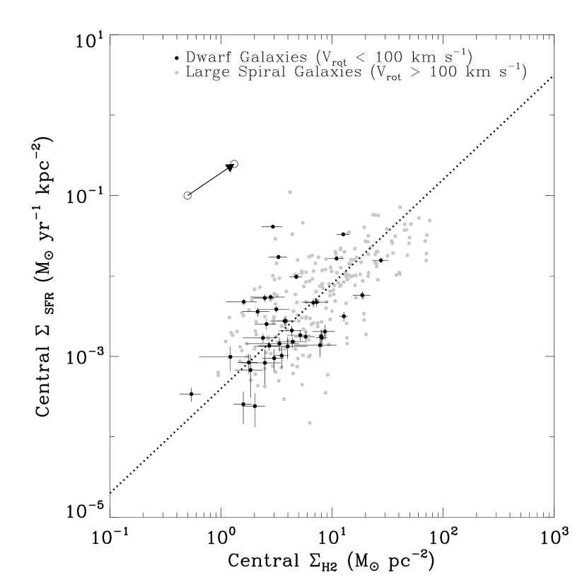
Figure 15.— The star formation surface density of spiral and irregular galaxies, derived from the 1.4 GHz radio continuum, plotted against the central surface density of molecular gas, derived from the integrated intensity of the CO line. Dwarf galaxies (those with $V_{\mbox{rot}}\leq 100$ km s^-1) are displayed as solid black circles, while large spiral galaxies are shown as gray circles. The Schmidt Law that best fits all galaxies is shown as a dotted line. The open circles connected by an arrow show the effect of a typical correction using Wilson (1995) and Bell (2003) as described in the text, but these corrections are not applied to the data in this plot. The sample of galaxies in this figure has been adjusted slightly from that in Figure 14. To create a homogeneous subsample free from spurious bulge contributions or inclination effects, we discarded all galaxies with Hubble Types earlier than Sb, inclinations $>85^{\circ}$ and angular diameters $>7^{\prime}$.

The slope derived here agrees within the uncertainties with that found by Kennicutt (1989), who used the total gas surface density ($\Sigma_{\rm HI}+\Sigma_{H2}$) rather than the molecular gas surface density. Dwarfs in our sample have ISMs dominated by atomic gas, so the agreement between these two indices using different gas surface densities bears investigating. However, we lack resolved atomic hydrogen observations of most of the dwarfs in our sample and therefore cannot further investigate the question of whether the atomic/total or molecular gas surface density is most relevant to star formation.

4.2. Molecular Gas Depletion Times and Star Formation Efficiency

Equations 12 and 13 can be adjusted to yield the depletion time, $\tau_{Dep}$ for molecular gas as a function of $\Sigma_{Mol}$:

$$\tau_{Dep}=2.5\times 10^{9}\Sigma_{Mol}^{-0.3}\mbox{ years}$$ (14)

with $\Sigma_{Mol}$ measured in M_⊙ pc^-2. The depletion time then is the time to consume all of the available molecular gas at the present rate of star formation. Because $\Sigma_{SFR}$ rises faster than $\Sigma_{Mol}$, the greater the surface density of molecular gas, the faster the gas is depleted. The median $\Sigma_{Mol}$ for a dwarf galaxy in our sample is $\sim 3$ M_⊙ pc^-2, which corresponds to a depletion time of $\approx 1.8\times 10^{9}$ years. For 10 M_⊙ pc^-2, a value typical for large spirals, $\tau_{Dep}$ drops to $\approx 1.25\times 10^{9}$ years. Strongly molecule-dominated galaxies, where $\Sigma_{Mol}\sim 300$ M_⊙ pc^-2, have $\tau_{Dep}\sim 4.5\times 10^{8}$ years.

The star formation efficiency (SFE) is often used to characterize star formation. The SFE can be defined as the fraction of molecular gas turned into stars over $10^{8}$ years. In this case SFE is proportional to the inverse of $\tau_{Dep}$ and equation 14 can be rearranged to yield

$$SFE=0.04\Sigma_{Mol}^{0.3}$$ (15)

with $\Sigma_{Mol}$ again in M_⊙ pc^-2. The SFE of a typical dwarf ($\Sigma_{Mol}=3$ M_⊙ pc^-2) is $\approx 0.056$ and that of a large spiral ($\Sigma_{Mol}=10$ M_⊙ pc^-2) is $\approx 0.08$.

Thus, although the two types of galaxy appear to obey the same underlying relationships, this does not imply that they exhibit the same SFE or $\tau_{Dep}$. Because dwarf galaxies tend to have lower average $\Sigma_{Mol}$ than large spirals, they exhibit slightly lower SFE and slightly larger $\tau_{Dep}$ than more massive systems. This explains the trend of decreasing $\tau_{Dep}$ with galaxy mass seen in Figure 10. The gradual upward trend among more massive galaxies is more puzzling. If real, it could be a result of a slight decrease in average molecular gas surface density with increasing galaxy mass, but we see no strong evidence such a decrease among the large galaxies in our sample. We also note that the depletion time for both types of galaxies is $\sim 10^{9}$ years, much less than a Hubble time. For star formation to be an ongoing process over a Hubble time in all of these systems, molecular gas must be continuously replenished.

4.3. Effects of the CO-to-H₂ and RC-to-SFR Conversion Factors

The results of the previous section are particularly surprising because it has often been suggested that in low metallicity environments like dwarf galaxies the CO-to-H₂ conversion factor, X_CO, may be much higher than the Galactic value (e.g., Maloney & Black, 1988). A number of studies of dwarf galaxies using virial methods have found values of X_CO that are larger than the Galactic value (Wilson, 1995; Arimoto, Sofue, & Tsujimoto, 1996; Mizuno et al., 2001a, b, and references therein). Far infrared studies also find large variations in X_CO with metallicity and radiation field (Israel, 1997). Recent applications of the virial method to nearby galaxies at higher resolutions and signal-to-noise ratios, though, find little evidence for changes in X_CO with environment (Rosolowsky et al., 2003; Walter et al., 2001, 2002; Bolatto et al., 2003). Though these new results for GMCs are compelling, their applicability to clouds other than massive GMCs is uncertain and the issue of the CO-to-H₂ calibration remains an open one.

The data shown in Figures 8 and 14 provides some constraint on variations in X_CO. If X_CO increases with decreasing metallicity, and the RC-to-SFR conversion does not change with metallicity, then the (black) data points in Figure 15 will move from left to right. If we assume that the underlying relationship between SFR and molecular gas is the same for large spirals and dwarf galaxies, then any variations in X_CO within the dwarfs in our sample would have to be small in order to maintain the agreement between dwarfs and large galaxies seen in Figure 14. Even if we allow the RC-to-SFR conversion vary with metallicity, to hide a change in X_CO of an order of magnitude over the range of metallicities of our sample requires changing the RC-to-SFR conversion by a similar factor, which appears very unlikely.

How much is the RC-to-SFR calibration likely to change over our sample? The conversion between RC and SFR relies on an empirical calibration of the nonthermal synchrotron emission to the supernova rate. Alternatively, the RC-to-SFR conversion can be calibrated via the FIR-to-RC correlation, since the FIR luminosity of a galaxy can be directly converted into a star formation rate once the amount of UV light reprocessed by dust is known. Both of these methods will break down when applied to sufficiently small objects. The fraction of relativistic electrons that escape from a galaxy is not well known, but cosmic rays may be more likely to escape from a small galaxy by diffusion or convection (e.g., Condon, 1992, and references therein). Therefore, a given amount of star formation could lead to less RC emission in dwarfs than in large galaxies. Similarly, small galaxies, with their shorter path lengths to escape and lower dust abundances, are likely to reprocess less of the UV photons emitted by young stars into FIR emission. Since the FIR and RC are strongly correlated down to luminosities of $L_{FIR}\sim 10^{8}L_{\odot}$ or lower, if FIR traces SFR nonlinearly then RC must also trace SFR nonlinearly (Bell, 2003). Although a thorough calibration effort of the RC-to-SFR relation for small systems has yet to be undertaken, this reasoning suggests that applying the RC-to-SFR calibration derived in the Milky Way or other large galaxies to smaller systems would yield SFRs that are too low.

To investigate the effects of possible changes in the CO-to-H₂ and RC-to-SFR calibrations in our derived star formation laws we apply to our sample some of the corrections suggested in the literature. We modified Equation 7 to include a luminosity correction, as suggested by Bell (2003),

$$\Sigma_{SFR}\left(\frac{M_{\odot}}{\mbox{yr kpc}^{2}}\right)=8.0\times 10^{-4}$$ (16)

$$\times F_{\nu,1.4}~{}\left(\mbox{mJy}\right)\,\left({\frac{\theta}{\mbox{45\arcsec}}}\right)^{-2}\frac{\cos i}{0.1+0.9\left(\frac{L}{L_{c}}\right)^{0.3}}\mbox{ .}$$

Here $L_{c}=6.4\times 10^{21}$ W Hz^-1, the approximate RC luminosity of an $L_{*}$ galaxy, and the correction applies only to galaxies with radio luminosities below $L_{c}$. This correction is obtained by comparing the RC to the infrared luminosity of a galaxy, which is in turn calibrated against its UV emission. Because smaller galaxies reprocess less of their UV light into infrared light, they have more star formation per unit infrared luminosity, thus the correction factor increases with decreasing galaxy luminosity (the connection to the RC is via the empirical FIR-to-RC correlation). To correct X_CO by metallicity effects we employ the dependence found by Wilson (1995)

$$\log\frac{X_{CO}}{X_{CO}^{MW}}={5.95-0.67\times[12+\log\mbox{(O/H)}}]$$

where we have estimated metallicities from the absolute B magnitudes of the dwarf galaxies using the relationship found by Richer & McCall (1995) given in Equation 4 above. We find that the power law that best describes the relationship between the adjusted $\Sigma_{SFR}$ and $\Sigma_{Mol}$ is

$$\Sigma_{SFR}^{\mathrm{Small}}=10^{-3.6\pm 0.3}\Sigma_{Mol}^{1.3\pm 0.3}$$ (17)

which agrees, within the uncertainties, with the uncorrected results.

After applying reasonable corrections to Equations 7 and 8, the actual values of both $\Sigma_{Mol}$ and $\Sigma_{SFR}$ have both increased by factors of $\sim 3$ for each dwarf galaxy, so that we derive the same underlying relationship between these two quantities. If we apply either correction without the other to the dwarf galaxies, we get a difference in the coefficients with no change in the exponent $b$ within the uncertainties ($\Sigma_{SFR}=10^{-4.0\pm 0.3}\Sigma_{Mol}^{1.4\pm 0.3}$ for only the X_CO correction, and $\Sigma_{SFR}=10^{-3.0\pm 0.2}\Sigma_{Mol}^{1.1\pm 0.4}$ for only the RC correction). Thus, if only one correction holds, dwarf galaxies form a different mass of stars per unit molecular gas than large galaxies — less if only X_CO is a strong function of metallicity, more if only the SFR.

Therefore, we find that the power law index relating $\Sigma_{Mol}$ to $\Sigma_{SFR}$ appears to be roughly the same, $\sim 1.1-1.4$, irrespective of mild changes in the assumed CO-to-H₂ and RC-to-SFR conversions. Plausible corrections to both the SFR and H₂ estimates based on the RC and the CO yields a Schmidt Law coefficient that is identical to that found with no corrections, implying that dwarf and large galaxies show the same star formation surface density for a given H₂ surface density. This result breaks down if only one of the SFR or the H₂ estimates are corrected. We do note that the majority of dwarf galaxies considered here are dwarf spirals. An extension of this analysis to dimmer dwarf irregular galaxies would probe a yet more extreme set of physical conditions and be of considerable interest, but this will require millimeter wave telescopes with increased sensitivity.

5. Summary and Conclusions

We report the detection of molecular gas in $28$ dwarf galaxies with no previously published CO detections and the marginal detection of $16$ more. We also present upper limits for $77$ dwarf galaxies that we did not detect. These data increase by more than 50% the number of published CO detections of dwarf galaxies. Most detections are late type spirals (Hubble type $\sim$Sc), of about the same stellar and dynamical mass of the Large Magellanic Cloud, with considerably brighter CO emission but somewhat lower star formation activity, and located at a distance of $\sim 11$ Mpc. Nondetected galaxies tend to be smaller than detections, with slightly later Hubble types (usually Irr).

The most significant differences between the detections and the nondetections appear to be the stellar mass, traced by $K$- and $B$-band luminosities, and high mass star formation rate, traced by their FIR emission and (less significantly) radio continuum luminosities. The correlations we observe between the presence of CO emission and other galaxy parameters, such as Hubble type or mass to light ratio can largely be ascribed to the fact that these properties are also correlated with luminosity. The tight correlation between the molecular gas mass and the $K$-band luminosity may result from the dominant role played by the stellar disk in setting the midplane pressure or equivalently local density of the atomic gas. Thus, dwarf galaxies tend to have roughly the same amount of molecular gas per unit stellar mass as large spirals, although their ISMs are dominated by large reservoirs of atomic gas and the molecular gas makes up only a small fraction of the total gas mass.

Given the distances to our targets and the sensitivity of our survey, we would not expect to detect galaxies with much less CO emission than the LMC. Thus, we do not know if these correlations hold for lower mass galaxies, but we see no evidence that we have “hit a wall” in our attempt to detect CO in small galaxies. Both our detections and the upper limits associated with our nondetections are consistent with a nearly constant $M_{Mol}/L_{\odot,K}\approx 0.075$ throughout our sample.

Because the nondetections include the most “primeval” (metal poor, low mass, and dynamically simple) galaxies in the sample, achieving the order of magnitude increase in sensitivity necessary to (perhaps) detect them in CO would be useful. If a change in CO properties exists, it may well be at very low metallicities where CO ceases to trace H₂. For instance, Taylor et al. (1998) suggested a sharp increase in the CO-to-H₂ conversion factor, X_CO  below $Z\approx 1/10Z_{\odot}$. Though we see a drop in detection rates with decreasing metallicity (traced by B-magnitude) within our own sample, the metallicity is covariant with many other galaxy properties and we find no evidence for substantial changes in X_CObetween $Z_{\odot}>Z>1/4Z_{\odot}$.

Combining our data with that of several previous CO surveys and the NVSS, we find that dwarf galaxies with detected CO emission show the same relationship between CO and the 1.4 GHz radio continuum as large galaxies. This result suggests that there is a constant star formation efficiency among dwarfs and large galaxies at a given $\Sigma_{H_{2}}$. This conclusion is insensitive to the application of small corrections to both the CO-to-H₂ and RC-to-SFR conversions, although not to either conversion factor alone. Apparently, changes of factors of $\sim 5$ in metallicity and galaxy stellar mass are not enough to markedly alter the $\Sigma_{SFR}$-to-$\Sigma_{Mol}$ relation.

Table 1 Table of CO Observations

Galaxy	RA	DEC	V${}_{\mbox{LSR}}$	M${}_{\mbox{B}}$	$\log$ L${}_{\mbox{FIR}}$	F1.4	V${}_{\mbox{rot}}$	I${}_{\mbox{CO}}$	Detected
	(J2000)	(J2000)	(km s-1)		(L⊙)	(mJy)	(km s-1)	(K km s-1)
NGC 14	00 08 46.2	15 48 55.4	864.4	-17.9	8.4	2.8	51.4	$\leq$ 0.63	N
NGC 100	00 24 02.7	16 29 11.3	842.0	-17.9	$\ldots$	$<1.0$	97.1	$\leq$ 0.44	N
UGC 1200	01 42 48.3	13 09 19.4	808.1	-16.2	$\ldots$	1.6	62.2	$\leq$ 0.81	N
IC 1727	01 47 29.9	27 19 59.1	346.4	-17.4	7.6	1.2	53.1	$\leq$ 0.60	N
UGC 1281	01 49 31.6	32 35 16.4	157.1	-15.8	$\ldots$	1.1	50.5	$\leq$ 0.80	N
NGC 784	02 01 16.7	28 50 14.2	197.6	-16.0	7.2	3.3	42.8	$\leq$ 0.76	N
NGC 949	02 30 48.8	37 08 12.1	611.1	-18.1	8.8	13.5	100.5	1.87 $\pm$ 0.32	Y
NGC 959	02 32 23.8	35 29 41.6	601.7	-17.3	8.3	3.0	73.8	0.86 $\pm$ 0.17	Y
UGC 2023	02 33 18.1	33 29 25.8	605.7	-16.4	7.8	$<1.0$	46.1	$\leq$ 0.75	N
UGC 2082	02 36 16.3	25 25 24.2	706.7	-18.0	8.0	1.4	86.1	1.24 $\pm$ 0.29	M
NGC 1012	02 39 14.9	30 09 05.0	978.3	-18.2	9.2	27.8	97.5	1.50 $\pm$ 0.29	Y
NGC 1036	02 40 29.1	19 17 49.2	785.0	-17.1	8.5	4.3	83.8	0.87 $\pm$ 0.17	Y
UGC 2259	02 47 55.5	37 32 17.5	584.9	-15.2	$\ldots$	$<1.0$	92.5	$\leq$ 0.82	N
NGC 1156	02 59 42.2	25 14 15.3	373.6	-17.6	8.5	12.1	57.1	0.76 $\pm$ 0.16	Y
NGC 1560	04 32 47.7	71 52 45.8	-36.9	-16.5	$\ldots$	3.3	76.2	1.36 $\pm$ 0.40	M
UGC 3137	04 46 15.6	76 25 06.6	992.3	-17.2	$\ldots$	$<1.0$	90.2	0.32 $\pm$ 0.11	M
UGCA 105	05 14 14.8	62 34 48.3	111.5	-15.3	$\ldots$	2.1	51.6	0.61 $\pm$ 0.16	M
UGC 3371	05 56 36.6	75 18 58.6	815.9	-16.9	$\ldots$	$<1.0$	82.6	$\leq$ 0.58	N
UGCA 130	06 42 15.5	75 37 24.9	792.9	-15.6	$\ldots$	$<1.0$	35.2	$\leq$ 1.00	N
NGC 2344	07 12 28.7	47 10 00.1	971.6	-18.3	8.4	1.8	153.8	1.24 $\pm$ 0.23	Y
NGC 2366	07 28 51.9	69 12 30.9	99.6	-16.8	8.1	2.4	42.9	$\leq$ 1.35	N
NGC 2500	08 01 52.8	50 44 14.9	512.0	-17.8	8.6	3.6	127.4	$\leq$ 1.09	N
UGC 4278	08 13 59.0	45 44 37.6	559.2	-18.2	7.8	$<1.0$	79.4	$\leq$ 0.56	N
NGC 2541	08 14 40.1	49 03 40.3	558.5	-18.2	8.5	1.6	93.1	$\leq$ 0.95	N
UGC 4305	08 19 03.9	70 43 08.7	157.9	-17.7	7.8	1.2	35.1	$\leq$ 1.32	N
NGC 2552	08 19 19.8	50 00 27.3	519.8	-17.5	8.0	$<1.0$	62.7	0.36 $\pm$ 0.10	M
UGC 4459	08 34 07.1	66 10 55.1	18.9	$\ldots$	$\ldots$	1.1	$\ldots$	$\leq$ 0.90	N
UGC 4499	08 37 41.4	51 39 09.7	691.7	-15.9	8.0	2.0	61.2	0.79 $\pm$ 0.23	M
UGC 4514	08 39 37.7	53 27 24.1	693.5	-16.3	7.9	1.1	72.6	$\leq$ 0.88	N
UGC 5151	09 40 27.1	48 20 13.5	776.0	-17.0	8.2	2.1	84.1	$\leq$ 1.17	N
UGC 5272	09 50 22.4	31 29 16.0	520.1	-15.3	7.5	2.0	38.5	$\leq$ 0.75	N
UGC 5414	10 03 57.0	40 45 20.8	610.2	-16.2	7.9	1.8	53.8	$\leq$ 0.72	N
UGC 5456	10 07 19.7	10 21 44.2	540.4	-15.7	7.8	1.3	31.0	$\leq$ 1.00	N
NGC 3239	10 25 05.4	17 09 43.9	753.4	-19.0	8.9	8.6	79.3	$\leq$ 0.53	N
IC 2574	10 28 21.5	68 24 41.0	47.4	-17.6	$\ldots$	$<1.0$	65.2	0.86 $\pm$ 0.17	Y
DDO 82	10 30 34.5	70 37 13.4	180.0	$\ldots$	$\ldots$	$<1.0$	$\ldots$	$\leq$ 0.96	N
NGC 3264	10 32 19.7	56 05 03.4	939.6	-18.2	8.3	2.1	53.3	$\leq$ 1.17	N
UGC 5829	10 42 42.1	34 26 56.0	624.7	-16.5	7.8	1.2	36.2	$\leq$ 1.20	N
NGC 3413	10 51 20.7	32 45 59.3	645.7	-17.7	8.3	4.7	72.3	$\leq$ 1.09	N
UGC 5986	10 52 30.9	36 37 08.7	615.5	-19.3	9.1	22.2	118.9	$\leq$ 0.81	N
NGC 3510	11 03 43.5	28 53 07.0	704.3	-16.7	8.2	3.1	83.2	$\leq$ 0.79	N
UGCA 225	11 04 58.2	29 08 17.1	645.8	-14.6	$\ldots$	2.0	38.5	$\leq$ 1.24	N
UGC 6446	11 26 40.4	53 44 48.4	644.3	-16.8	$\ldots$	$<1.0$	80.2	$\leq$ 0.54	N
UGC 6448	11 26 50.3	64 08 19.6	989.6	-16.3	8.2	$<1.0$	38.5	$\leq$ 0.65	N
UGC 6456	11 27 58.8	78 59 38.4	-93.4	-11.2	$\ldots$	1.2	20.7	$\leq$ 0.99	N
NGC 3773	11 38 12.9	12 06 43.5	975.6	-16.9	8.6	5.6	74.3	$\leq$ 1.01	N
NGC 3782	11 39 20.5	46 30 51.4	737.1	-17.6	8.6	4.6	64.9	1.19 $\pm$ 0.33	M
UGC 6628	11 40 05.7	45 56 32.6	849.8	-17.6	8.1	$<1.0$	25.6	$\leq$ 0.60	N
NGC 3870	11 45 56.6	50 11 57.4	755.0	-17.3	8.6	4.8	67.6	0.52 $\pm$ 0.11	Y
NGC 3906	11 49 40.9	48 25 34.3	950.9	-17.3	8.4	2.0	127.6	0.59 $\pm$ 0.18	M
NGC 3913	11 50 38.9	55 21 13.6	954.0	-17.8	8.4	$<1.0$	34.8	1.98 $\pm$ 0.24	Y
UGC 6900	11 55 39.0	31 31 07.6	589.6	-15.5	$\ldots$	$<1.0$	48.5	$\leq$ 0.81	N
UGC 6917	11 56 27.7	50 25 43.6	911.2	-18.1	8.2	1.1	91.8	$\leq$ 1.29	N
NGC 3985	11 56 42.0	48 20 01.6	947.3	-18.1	8.8	6.5	84.3	0.88 $\pm$ 0.19	Y
NGC 3990	11 57 35.6	55 27 29.1	695.0	$\ldots$	$\ldots$	$<1.0$	$\ldots$	$\leq$ 1.12	N
NGC 4068	12 04 01.0	52 35 16.4	210.2	-15.0	7.3	$<1.0$	27.1	0.68 $\pm$ 0.18	M
NGC 4080	12 04 51.8	26 59 33.3	585.7	-16.2	7.8	1.7	82.2	1.88 $\pm$ 0.43	Y
NGC 4136	12 09 17.7	29 55 41.1	607.7	-17.5	8.5	$<1.0$	93.3	1.59 $\pm$ 0.25	Y
NGC 4144	12 09 58.6	46 27 27.0	267.1	-17.6	8.1	4.9	76.0	1.06 $\pm$ 0.22	Y
NGC 4150	12 10 33.6	30 24 05.7	226.0	$\ldots$	7.8	1.4	$\ldots$	2.38 $\pm$ 0.42	Y
NGC 4190	12 13 44.1	36 37 53.7	230.0	-15.0	7.4	4.6	50.5	$\leq$ 1.28	N
UGC 7261	12 15 14.3	20 39 32.0	838.0	-16.8	8.4	1.0	68.4	$\leq$ 0.63	N
NGC 4218	12 15 46.1	48 07 54.1	724.8	-16.9	8.5	4.9	69.2	$\leq$ 0.95	N
NGC 4299	12 21 40.4	11 30 10.8	231.1	-15.4	$\ldots$	10.1	122.7	$\leq$ 0.77	N
NGC 4309	12 22 12.3	07 08 39.1	871.7	-16.6	8.4	2.3	109.4	3.01 $\pm$ 0.54	Y
NGC 4310	12 22 26.3	29 12 29.8	887.1	-17.4	8.6	2.2	78.9	3.31 $\pm$ 0.52	Y
UGC 7490	12 24 24.7	70 20 02.0	466.7	-16.4	7.8	$<1.0$	36.1	$\leq$ 1.10	N
NGC 4395	12 25 49.0	33 32 49.2	319.7	-18.0	$\ldots$	2.1	57.4	$\leq$ 0.93	N
NGC 4396	12 25 59.1	15 40 15.5	-124.6	$\ldots$	5.3	8.8	81.8	2.37 $\pm$ 0.48	Y
UGC 7559	12 27 04.7	37 08 38.7	218.1	-14.7	$\ldots$	$<1.0$	30.1	$\leq$ 0.98	N
UGC 7557	12 27 11.3	07 15 44.9	932.9	-17.8	8.0	1.9	63.8	$\leq$ 0.87	N
UGC 7599	12 28 28.1	37 14 00.6	277.8	-14.2	$\ldots$	$<1.0$	29.8	$\leq$ 1.27	N
UGC 7603	12 28 44.0	22 49 17.0	642.1	-16.7	8.0	1.9	51.2	$\leq$ 0.69	N
IC 3414	12 29 29.0	06 46 16.6	537.1	-15.6	7.5	$<1.0$	52.7	$\leq$ 2.27	N
UGC 7690	12 32 26.8	42 42 18.0	537.4	-16.9	8.0	1.6	71.8	$\leq$ 0.99	N
UGC 7698	12 32 54.4	31 32 30.8	332.7	-16.2	$\ldots$	1.1	29.1	$\leq$ 0.80	N
NGC 4509	12 33 06.7	32 05 27.9	935.1	-15.8	8.3	2.8	40.9	$\leq$ 1.25	N
NGC 4534	12 34 05.4	35 31 05.1	801.9	-17.8	8.4	2.0	74.8	$\leq$ 1.40	N
NGC 4618	12 41 32.5	41 08 57.1	543.1	-18.8	8.9	6.6	67.6	1.23 $\pm$ 0.21	Y
NGC 4625	12 41 52.6	41 16 27.1	610.6	-17.3	8.5	3.5	47.4	2.26 $\pm$ 0.26	Y
NGC 4630	12 42 31.1	03 57 33.1	738.7	-17.1	8.7	8.2	75.9	4.45 $\pm$ 0.38	Y
NGC 4633	12 42 37.0	14 21 19.8	290.3	-15.4	$\ldots$	2.0	91.4	$\leq$ 0.94	N
NGC 4635	12 42 39.2	19 56 43.0	960.0	-17.9	8.4	1.1	101.4	1.71 $\pm$ 0.29	Y
UGCA 294	12 44 38.1	28 28 21.3	944.9	-15.4	$\ldots$	$<1.0$	42.1	$\leq$ 0.59	N
IC 3742	12 45 31.7	13 19 51.9	964.7	-17.2	8.1	$<1.0$	81.3	$\leq$ 0.78	N
UGCA 298	12 46 55.3	26 33 51.4	830.2	$\ldots$	$\ldots$	$<1.0$	$\ldots$	$\leq$ 1.07	N
NGC 4688	12 47 46.5	04 20 08.1	986.3	-17.4	8.6	1.9	60.1	$\leq$ 1.20	N
NGC 4701	12 49 11.6	03 23 18.9	723.1	-17.5	8.8	11.9	108.4	4.85 $\pm$ 0.56	Y
NGC 4713	12 49 57.6	05 18 41.4	652.2	-17.9	8.9	18.5	119.4	3.61 $\pm$ 0.39	Y
NGC 4765	12 53 14.6	04 27 46.7	724.5	-17.0	8.6	14.4	51.4	0.85 $\pm$ 0.26	M
UGC 8146	13 02 07.8	58 42 00.0	668.8	-16.7	$\ldots$	$<1.0$	77.1	$\leq$ 1.27	N
UGC 8246	13 10 04.3	34 10 49.4	799.5	-16.4	7.9	$<1.0$	62.7	$\leq$ 1.05	N
IC 4213	13 12 11.1	35 40 18.1	814.8	-17.6	8.0	1.0	81.7	0.84 $\pm$ 0.20	Y
DDO 166	13 13 17.8	36 12 56.5	945.5	-17.3	8.3	$<1.0$	52.1	2.01 $\pm$ 0.48	M
UGC 8320	13 14 27.8	45 55 11.2	194.4	-16.2	$\ldots$	1.3	50.1	$\leq$ 0.97	N
UGC 8323	13 14 48.4	34 52 51.6	858.3	-16.3	8.2	2.1	50.2	$\leq$ 1.54	N
NGC 5107	13 21 24.5	38 32 18.6	945.6	-17.2	8.6	3.6	67.8	$\leq$ 0.87	N
UGC 8490	13 29 36.4	58 25 12.7	202.9	-17.5	8.3	3.6	58.3	$\leq$ 0.78	N
UGC 8507	13 30 58.6	19 26 11.4	999.2	-17.3	8.1	1.0	44.8	$\leq$ 1.08	N
NGC 5238	13 34 42.5	51 36 48.5	233.0	-14.9	$\ldots$	$<1.0$	21.6	$\leq$ 1.01	N
NGC 5338	13 53 26.5	05 12 27.3	815.8	-16.6	8.0	1.1	32.7	0.97 $\pm$ 0.18	Y
NGC 5474	14 05 01.5	53 39 44.2	276.3	-17.6	8.2	1.8	22.1	$\leq$ 0.40	N
NGC 5477	14 05 33.1	54 27 40.3	305.0	-14.9	7.5	$<1.0$	30.9	$\leq$ 0.97	N
NGC 5585	14 19 47.6	56 43 44.7	304.9	-18.2	8.2	2.5	96.8	$\leq$ 0.99	N
UGC 9405	14 35 24.5	57 15 16.5	221.1	$\ldots$	$\ldots$	$<1.0$	36.2	$\leq$ 0.57	N
NGC 5832	14 57 45.7	71 40 53.0	448.9	-16.3	8.0	2.7	74.5	1.20 $\pm$ 0.29	M
NGC 5949	15 28 00.6	64 45 47.8	429.8	-17.1	8.4	3.4	88.3	1.86 $\pm$ 0.51	M
NGC 5963	15 33 27.7	56 33 32.7	655.1	-17.8	8.8	6.5	121.1	2.29 $\pm$ 0.30	Y
UGCA 410	15 37 04.1	55 15 48.6	660.8	-15.3	$\ldots$	$<1.0$	61.5	$\leq$ 0.93	N
UGC 10310	16 16 18.1	47 02 44.5	713.8	-17.1	8.0	$<1.0$	55.8	$\leq$ 0.76	N
UGC 10445	16 33 47.7	28 59 05.2	961.8	-17.3	8.4	$<1.0$	82.4	0.60 $\pm$ 0.17	M
NGC 6255	16 54 47.3	36 30 05.3	915.3	-17.8	8.4	1.2	98.6	$\leq$ 1.13	N
UGC 10806	17 18 51.3	49 53 02.3	929.5	-17.4	8.4	2.3	71.1	$\leq$ 0.75	N
NGC 6689	18 34 49.8	70 31 28.9	489.2	-17.9	8.3	1.8	91.0	1.49 $\pm$ 0.28	Y
NGC 6789	19 16 41.6	63 58 22.4	-148.5	$\ldots$	$\ldots$	$<1.0$	$\ldots$	1.04 $\pm$ 0.27	M
UGC 11891	22 03 33.7	43 44 56.7	461.4	-16.1	$\ldots$	1.2	86.9	0.33 $\pm$ 0.11	M
NGC 7292	22 28 25.9	30 17 28.6	985.6	-18.1	8.7	5.0	44.2	$\leq$ 0.77	N
UGC 12060	22 30 33.6	33 49 17.0	884.0	-15.5	$\ldots$	$<1.0$	52.5	1.12 $\pm$ 0.18	Y
DDO 213	22 34 10.8	32 51 41.0	804.7	-16.9	$\ldots$	$<1.0$	52.4	$\leq$ 0.81	N
UGC 12632	23 29 58.7	40 59 25.4	422.2	-17.4	$\ldots$	$<1.0$	79.3	$\leq$ 0.71	N
UGC 12732	23 40 39.9	26 14 10.3	748.5	-16.5	$\ldots$	$<1.0$	95.1	$\leq$ 0.68	N

Table 2 Rank Correlations Between CO and other Galaxy Properties

Property	with $M_{Mol}$	with $M_{Mol}/L_{K}$	with $M_{Mol}/L_{B}$	with $M_{Mol}/M_{dyn}$	with $M_{Mol}/M_{HI}$	with $M_{Mol}/L_{RC}$	with $M_{Mol}/L_{FIR}$
	Molecular Gas	Molecular Gas		Molecular Gas	Molecular Gas	Molecular Gas
	Mass	per unit		per unit	to Atomic Gas	Depletion Time
		Stellar Mass		Dynamical Mass	Ratio
Biases
Virgocentric Velocity/Distance	+0.62	$+0.37$	$+0.38$	$+0.41$	$+0.32$	$\cdots$	$\cdots$
Angular Size	$\cdots$	$-0.42$	-0.35	$-0.39$	$\cdots$	$\cdots$	$\cdots$
Global Quantities
Hubble Type	$-0.49$	$\cdots$	$-0.26$	$\cdots$	-0.55	$\cdots$	$\cdots$
Dynamical Mass	$+0.69$	$\cdots$	$\cdots$	$\cdots$	$+0.36$	$\cdots$	$+0.30$
K-band Luminosity	+0.85	$\cdots$	$+0.26$	$\cdots$	$+0.50$	$\cdots$	$+0.30$
B-band Luminosity	+0.79	$\cdots$	$\cdots$	$\cdots$	$+0.41$	$\cdots$	$+0.29$
Linear Diameter	+0.68	$\cdots$	$\cdots$	$\cdots$	$+0.22$	$\cdots$	$+0.26$
FIR Luminosity	+0.90	$+0.47$	$+0.57$	$+0.55$	$+0.60$	$-0.42$	$\cdots$
RC Luminosity	+0.86	$+0.35$	$+0.45$	$+0.43$	$+0.53$	$-0.48$	$\cdots$
HI Luminosity	$+0.55$	$\cdots$	$\cdots$	$\cdots$	(-0.12)	$\cdots$	$\cdots$
Colors
$B-V$	$+0.35$	$\cdots$	$\cdots$	$\cdots$	$+0.53$	$\cdots$	$+0.35$
$B-K$	$+0.46$	$\cdots$	+0.56	$+0.31$	$+0.57$	$\cdots$	$\cdots$
FIR (60 $\mu$m) / FIR (100 $\mu$m)	$\cdots$	$+0.42$	$+0.40$	$+0.46$	$+0.31$	$-0.55$	$-0.35$
$M_{HI}/L_{B}$	$-0.42$	$\cdots$	$\cdots$	$\cdots$	$\cdots$	$\cdots$	$-0.24$
$M_{HI}/L_{K}$	$-0.50$	$\cdots$	-0.30	$\cdots$	$\cdots$	$\cdots$	$-0.25$
$M_{dyn}/L_{B}$	$\cdots$	$\cdots$	$\cdots$	$\cdots$	$\cdots$	$\cdots$	$\cdots$
$M_{dyn}/L_{K}$	-0.28	$\cdots$	$-0.27$	$\cdots$	$-0.32$	$+0.23$	$\cdots$
Median Values	$M_{\odot}$	$M_{\odot}/L_{K,\odot}$	$M_{\odot}/L_{B,\odot}$	$M_{\odot}/M_{\odot}$	$M_{\odot}/M_{\odot}$	$M_{\odot}/L_{\nu,1.4}(10^{12}\mathrm{W~{}Hz}^{-1})$	$M_{\odot}/L_{\odot}$
Dwarfs	$3\pm 0.5\times 10^{8}$	$0.065\pm 0.008$	$0.13\pm 0.02$	$0.037\pm 0.007$	$0.30\pm 0.05$	$1.4\pm 0.2$	$0.47\pm 0.08$
Large Spirals	$5\pm 0.5\times 10^{9}$	$0.075\pm 0.005$	$0.16\pm 0.01$	$0.040\pm 0.003$	$1.5\pm 0.1$	$1.0\pm 0.05$	$0.64\pm 0.03$

Note. — This table shows rank correlation coefficients for a combined sample of large spirals and dwarf galaxies. Typical $1\sigma$ uncertainties for the values in this table are $\pm 0.07$. Only Values significant at $>3\sigma$ level are shown.

Table 3 Power Law Relations Between CO and other Galaxy Properties

Property	Exponent		Scatter About Best Fit (dex)
	$\overbrace{\phantom{string}}$		$\overbrace{\phantom{string}}$
	All Galaxies	Dwarfs	All Galaxies	Dwarfs
Dynamical Mass	$1.2\pm 0.2$	$\cdots$	0.6	0.6
K-band Luminosity	$1.2\pm 0.1$	$1.3\pm 0.2$	0.4	0.4
B-band Luminosity	$1.2\pm 0.3$	$1.3\pm 0.2$	0.5	0.5
FIR Luminosity	$1.1\pm 0.1$	$1.0\pm 0.3$	0.4	0.5
RC Luminosity	$0.8\pm 0.1$	$0.9\pm 1.6$	0.4	0.6

Table 4 Median Detection/Nondetection Properties

Property	Median Detection Value	Median Nondetection Value
Biases
Virgocentric Velocity Distance	$11.3\pm 0.6$ Mpc	$10.9\pm 0.5$ Mpc
RMS Noise	$7.7\pm 0.4$ mK	$8.3\pm 0.2$ mK
Angular Size	$2.4^{\prime}\pm 0.8$	$2.7^{\prime}\pm 0.2$
Global Quantities
Hubble Type	$\sim$ Sc	Sm/Irr
Dynamical Mass ($\frac{V^{2}R}{G}$)	$8\pm 1\times 10^{9}$ M⊙	$3\pm 1\times 10^{9}$ M⊙
Absolute K Magnitude	$-20.4\pm 0.2$	$-19.5\pm 0.2$
Absolute B Magnitude	$-17.6\pm 0.1$	$-16.8\pm 0.2$
Linear Diameter ($d_{25}$	$8.5\pm 0.8$ kpc	$7.7\pm 0.7$ kpc
$L_{FIR}$	$3.2\pm 0.6\times 10^{8}L_{\odot}$	$1.5\pm 0.2\times 10^{8}L_{\odot}$
$L_{RC}$	$13\pm 2\times 10^{19}$ W Hz-1	$5\pm 1\times 10^{19}$ W Hz-1
$M_{HI}$	$9\pm 2\times 10^{8}$ M⊙	$8\pm 1\times 10^{8}$ M⊙
Colors
$B-V$	$0.48\pm 0.03$	$0.43\pm 0.02$
$B-K$	$2.8\pm 0.1$	$2.1\pm 0.1$
FIR (60 $\mu$m) / FIR (100 $\mu$m)	$0.40\pm 0.02$	$0.41\pm 0.02$
$M_{HI}/L_{B}$	$0.40\pm 0.06$ M⊙/$L_{B\odot}$	$0.87\pm 0.09$ M⊙/$L_{B\odot}$
$M_{HI}/L_{K}$	$0.24\pm 0.04$ M⊙/$L_{K\odot}$	$0.77\pm 0.18$ M⊙/$L_{K\odot}$
$M_{dyn}/L_{B}$	$4.5\pm 0.8$	$3.8\pm 0.3$
$M_{dyn}/L_{K}$	$2.2\pm 0.3$	$4.2\pm 0.8$
CO Properties
LCO	$1.9\pm 0.6\times 10^{7}$ K km s-1 pc2	$<6.9\times 10^{6}$ K km s-1 pc2 ($2\sigma$)
MMol	$8.2\pm 2.6\times 10^{7}$ M⊙	$<3.0\times 10^{7}$ M⊙ (2$\sigma$)
Molecular Gas Surface Density	$3.1\pm 0.6$ M⊙ pc-2	$<1.6$ M⊙ pc-2 ($2\sigma$)

Table 5 Differences Between Detections and Nondetections

Property	KS Significance	Student’s t Significance
Biases
Virgocentric Velocity/Distance	0.35	0.67
Angular Size	0.68	0.88
RMS Noise in CO Spectrum	0.69	0.35
Global Quantities
Hubble Type	0.01	0.01
Dynamical Mass	0.03	0.02
Absolute K Magnitude	$\sim 10^{-4}$	$\sim 10^{-6}$
Absolute B Magnitude	0.001	0.001
Linear Diameter	0.44	0.88
$L_{FIR}$	$\sim 10^{-4}$	$\sim 10^{-4}$
$L_{RC}$	0.03	0.03
$M_{HI}$	0.58	0.46
Colors
$B-V$	0.34	0.14
$B-K$	0.001	$\sim 10^{-4}$
FIR (60 $\mu$m) / FIR (100 $\mu$m)	0.55	0.28
$M_{HI}/L_{B}$	$\sim 10^{-4}$	$\sim 10^{-6}$
$M_{HI}/L_{K}$	$\sim 10^{-4}$	$\sim 10^{-5}$
$M_{dyn}/L_{B}$	0.31	0.50
$M_{dyn}/L_{K}$	0.05	0.03

References

- Adler, Lo, & Allen (1991) Adler, D. S., Lo, K. Y., & Allen, R. J. 1991, ApJ, 382, 475
- Arimoto, Sofue, & Tsujimoto (1996) Arimoto, N., Sofue, Y., & Tsujimoto, T. 1996, PASJ, 48, 275
- Bell (2003) Bell, E. F. 2003, ApJ, 586, 794
- Blanton et al. (2003) Blanton, M. R., et al. 2003, ApJ, 594, 186
- Blitz & Rosolowsky (2004) Blitz, L. & Rosolowsky, E. 2004, ApJ, 612, L29
- Böker, Lisenfeld, & Schinnerer (2003) Böker, T., Lisenfeld, U., & Schinnerer, E. 2003, A&A, 406, 87
- Bolatto et al. (2003) Bolatto, A. D., Leroy, A., Israel, F. P., & Jackson, J. M. 2003, ApJ, 595, 167
- Condon (1992) Condon, J. J. 1992, ARA&A, 30, 575
- Condon et al. (1998) Condon, J. J., Cotton, W. D., Greisen, E. W., Yin, Q. F., Perley, R. A., Taylor, G. B., & Broderick, J. J. 1998, AJ, 115, 1693
- de Vaucouleurs et al. (1991) de Vaucouleurs, G., de Vaucouleurs, A., Corwin, H. G., Buta, R. J., Paturel, G., & Fouque, P. 1991, S&T, 82, 621
- Elfhag et al. (1996) Elfhag, T., Booth, R. S., Hoeglund, B., Johansson, L. E. B., & Sandqvist, A. 1996, A&AS, 115, 439
- Engargiola et al. (2003) Engargiola, G., Plambeck, R. L., Rosolowsky, E., & Blitz, L. 2003, ApJS, 149, 343
- Freedman et al. (2001) Freedman, W. L., et al. 2001, ApJ, 553, 47
- Fukui et al. (2001) Fukui, Y., Mizuno, N., Yamaguchi, R., Mizuno, A., & Onishi, T. 2001, PASJ, 53, L41
- Heyer et al. (2001) Heyer, M. H., Carpenter, J. M., & Snell, R. L. 2001, ApJ, 551, 852.
- Hollenbach, Werner, & Salpeter (1971) Hollenbach, D. J., Werner, M. W., & Salpeter, E. E. 1971, ApJ, 163, 165
- Isobe et al. (1990) Isobe, T., Feigelson, E. D., Akritas, M. G., & Babu, G. J. 1990, ApJ, 364, 104
- Israel & Burton (1986) Israel, F. P. & Burton, W. B. 1986, A&A, 168, 369
- Israel, Tacconi, & Baas (1995) Israel, F. P., Tacconi, L. J., & Baas, F. 1995, A&A, 295, 599
- Israel (1997) Israel, F. P. 1997, A&A, 328, 471
- Jarrett et al. (2000) Jarrett, T. H., Chester, T., Cutri, R., Schneider, S., Skrutskie, M., & Huchra, J. P. 2000, AJ, 119, 2498
- Kennicutt (1989) Kennicutt, R. C. 1989, ApJ, 344, 685
- Kim et al. (1998) Kim, S., Staveley-Smith, L., Dopita, M. A., Freeman, K. C., Sault, R. J., Kesteven, M. J., & McConnell, D. 1998, ApJ, 503, 674
- Kregel, van der Kruit, & de Grijs (2002) Kregel, M., van der Kruit, P. C., & de Grijs, R. 2002, MNRAS, 334, 646
- Lamareille et al. (2004) Lamareille, F., Mouhcine, M., Contini, T., Lewis, I., & Maddox, S. 2004, MNRAS, 350, 396
- Loinard & Allen (1998) Loinard, L. & Allen, R. J. 1998, ApJ, 499, 227
- Maloney & Black (1988) Maloney, P. & Black, J. H. 1988, ApJ, 325, 389
- Melisse & Israel (1994) Melisse, J. P. M. & Israel, F. P. 1994, A&AS, 103, 391
- Mizuno et al. (2001a) Mizuno, N. et al. 2001, PASJ, 53, 971 (2001a)
- Mizuno et al. (2001b) Mizuno, N. et al. 2001, PASJ, 53, L45 (2001b)
- Moshir et al. (1990) Moshir, M. & et al. 1990, IRAS Faint Source Catalogue, version 2.0 (1990)
- Murgia et al. (2002) Murgia, M., Crapsi, A., Moscadelli, L., & Gregorini, L. 2002, A&A, 385, 412
- Press et al. (1992) Press, W.H., S.A. Teukolsky, W.T. Vetterling, and B.P. Flannery, Numerical Recipes in C: The Art of Scientific Computing, 2nd ed., Cambridge Univ. Press, New York, 1992.
- Rand, Lord, & Higdon (1999) Rand, R. J., Lord, S. D., & Higdon, J. L. 1999, ApJ, 513, 720
- Regan & Vogel (1994) Regan, M. W. & Vogel, S. N. 1994, ApJ, 434, 536
- Richer & McCall (1995) Richer, M. G. & McCall, M. L. 1995, ApJ, 445, 642
- Rosolowsky et al. (2003) Rosolowsky, E., Plambeck, D., Engargiola, G., & Blitz, L. 2002, ApJ, in press
- Sakai et al. (2000) Sakai, S., et al.2000, ApJ, 529, 698
- Sauvage, Vigroux, & Thuan (1990) Sauvage, M., Vigroux, L., & Thuan, T. X. 1990, A&A, 237, 296
- Schlegel, Finkbeiner, & Davis (1998) Schlegel, D. J., Finkbeiner, D. P., & Davis, M. 1998, ApJ, 500, 525
- Shostak & van der Kruit (1984) Shostak, G. S. & van der Kruit, P. C. 1984, A&A, 132, 20
- Skillman, Côté, & Miller (2003) Skillman, E. D., Côté, S., & Miller, B. W. 2003, AJ, 125, 610
- Solomon et al. (1987) Solomon, P. M., Rivolo, A. R., Barrett, J., & Yahil, A. 1987, ApJ, 319, 730.
- Stanimirović, Staveley-Smith, & Jones (2004) Stanimirović, S., Staveley-Smith, L., & Jones, P. A. 2004, ApJ, 604, 176
- Strong & Mattox (1996) Strong, A. W. & Mattox, J. R. 1996, A&A, 308, L21
- Swaters et al. (2002) Swaters, R. A., van Albada, T. S., van der Hulst, J. M., & Sancisi, R. 2002, A&A, 390, 829
- Taylor, Kobulnicky, & Skillman (1998) Taylor, C. L., Kobulnicky, H. A., & Skillman, E. D. 1998, AJ, 116, 2746
- Walter et al. (2001) Walter, F., Taylor, C. L., Huttemeister, S., Scoville, N., & McIntyre, V. 2001, AJ, 121, 727.
- Walter et al. (2002) Walter, F., Weiss, A., Martin, C., & Scoville, N. 2002, AJ, 123, 225.
- Wilson (1995) Wilson, C. D. 1995, ApJ, 448, L97.
- Wong & Blitz (2002) Wong, T. & Blitz, L. 2002, ApJ, 569, 157
- Young & Scoville (1991) Young, J. S. & Scoville, N. Z. 1991, ARA&A, 29, 581
- Young et al. (1995) Young, J. S. et al. 1995, ApJS, 98, 219.
- Young (1999) Young, J. S. 1999, ApJ, 514, L87