Fast identification of transits from light-curves

Abstract

We present an algorithm that allows fast and efficient detection of transits, including planetary transits, from light-curves. The method is based on building an ensemble of fiducial models and compressing the data using the MOPED algorithm. We describe the method and demonstrate its efficiency by finding planet-like transits in simulated Pan-STARRS light-curves. We show that that our method is independent of the size of the search space of transit parameters. In large sets of light-curves, we achieve speed up factors of order of $10^{8}$ times over the full $\chi 2$ search. We discuss how the algorithm can be used in forthcoming large surveys like Pan-STARRS and LSST and how it may be optimized for future space missions like Kepler and COROT where most of the processing must be done on board.

1 Introduction

If the orbit of a planet around a star is so favorably inclined that $\sin(i)\approx 1$, the planet will transit the disk of the star once per orbit. During the transit the observed flux from the star is reduced by the ratio of the areas of the planet and the star, typically $\sim 1$% for a Jupiter-like planet around a Sun-like star. When this photometric dimming is observed to repeat periodically, a small radius companion may be inferred to exist. This effect is seen in star HD209458 (Charbonneau et al., 2000), which was first identified as a planetary system using the radial velocity technique. The added value of the detection of transits is great: not only is the $\sin(i)$ ambiguity resolved, but the radius of the planet may be inferred, and spectroscopic examination of the object during transit allows the study of the atmosphere of the planet (Charbonneau et al., 2002).

The transit technique to search for planets has some advantages: photometry is less costly in telescope time than spectroscopy, and one knows $\sin(i)$ for all the systems found this way. The major disadvantage is that the yield is comparatively low, since only systems with $\sin(i)\approx 1$ will be detected.

A large number of transit searches for extra-solar planets, both space-based and ground-based, have been completed or are underway (Gilliland, 2000; Mochejska et al., 2002; Udalski et al., 2002, 2003; Mallén-Ornelas et al., 2003). Many of these efforts employ small-aperture, wide-field cameras to monitor tens of thousands of nearby, bright stars. Of the surveys using this approach, the only success to date has come from the Trans-atlantic Exoplanet Survey (TrES), which recently announced the discovery of a planet dubbed TrES-1 (Alonso et al., 2004). The only other success (albeit for fainter stars where follow-up is more difficult) has come from the OGLE survey (Udalski et al., 2002, 2003). The vast majority of transits have been false detections resulting from grazing transits of stellar companions or a blend of an eclipsing binary with a brighter foreground or background star (Torres et al., 2004; Pont et al., 2005). Some progress has been made at differentiating these from planets (Hoekstra et al., 2005). However, the few candidates not eliminated by follow up studies, in particular OGLE-TR-56b with its 1.2-day orbital period, further challenge our already revised models of planet formation (Konacki et al., 2003).

The detection of a weak, short, periodic transit in noisy light-curves is a challenging task. The large number of light-curves collected make automation and optimization processes a necessity. This requirement is even stronger in the context of space missions where much of the processing must be done on board. A number of transit-detection algorithms have been implemented in the literature (Doyle et al., 2000; Defaÿ, Deleuil, & Barge, 2001; Aigrain & Favata, 2002; Jenkins et al., 2002; Kovács et al., 2002; Udalski et al., 2002; Street et al., 2003) and there has been some effort to compare their perspective performances (Tingley, 2003) .

Such transit searches are generally performed by comparing light-curves to a family of models with a common set of parameters: the transit period $T$, the transit duration $\eta$, the epoch $\tau$ (which is equal to the time $t$ at the start of the first transit) and the transit depth $\theta$. The best set of parameters is identified by finding the model most likely to have given rise to the observed data, i.e. the model with the highest likelihood $L$. This is exactly the kind of problem MOPED (Heavens et al., 2000) was designed to address. In particular, light-curves contain plenty of redundant information: the light between transits. By using MOPED one can weigh more the part of the light-curve that is sensitive to the transit thus constructing one eigenvector for each of the parameters in the transit model. However, for the case of transit detection in light-curves, the MOPED eigenvectors are sensitive to the fiducial model, thus incorrectly overweighs some data . In this paper we present a solution to this problem by building an ensemble of fiducial models. We find that for each model in an ensemble of fiducial models, there are many possible solutions. However, only one solution is common to all models in the ensemble of fiducial models: the one with the correct parameter values of the transit. We construct a new statistical measure to determine for the set of fiducial models the correct value of the parameters for the transit. We also show that our algorithm passes the null test, i.e. it correctly identifies a light-curve with no transit. The set of fiducial models can be pre-computed and we provide a recipe to do this. We show that this needs to be done only once before the search for transits is performed in a set of light-curves.

The speed up in the analysis is significant. For a simulated light-curve typical of Pan-STARRS we find that our algorithm is $10^{8}$ times faster than a search in the full $\chi 2$ space. The speed up is due to the fact that using MOPED the maximum likelihood search is performed on four data (the number of parameters) instead of thousands and that the ensemble of fiducial models can be pre-computed. This achieved increase in speed to compute the likelihood is important for transit analysis since the likelihood surface has multiple maxima, of which only one is the desired solution and therefore the search for this best solution needs to explore the whole likelihood surface

This paper is organized as follows: In Section 2, we briefly describe MOPED. Section 3 presents the transit model used and how a set of synthetic light-curves were constructed. In Section 4, we describe the extension of MOPED using an ensemble of fiducial models and we also present how the results should be compared to the null hypothesis. Results are discussed in Section 5 and our conclusions summarized in Section 7. In Section 6, we describe the numerical topics including a numerical recipe.

2 MOPED

We briefly review the parameter estimation and data compression method MOPED which is originally described in Heavens et al. (2000). The method is as follows: given a set of data x (in our case a light-curve) which includes a signal part $\mu$ and noise ${\bf n}$, i.e.

$${\bf x}=\mbox{\boldmath$\mu$}+{\bf n},$$ (1)

the idea then is to find weighting vectors ${\bf b}_{m}$ where $m$ runs from 1 to the number of parameters $M$, such that

$$y_{m}\equiv\bf{b}_{m}\bf{x}$$ (2)

contain as much information as possible about the parameters (period, duration of the transit etc.). These numbers $y_{m}$ are then used as the data set in a likelihood analysis with the consequent increase in speed at finding the best solution. In MOPED, there is one vector associated with each parameter.

In Heavens et al. (2000) an optimal and lossless method was found to calculate ${\bf b}_{m}$ for multiple parameters (as is the case with transits). The definition of lossless here is that the Fisher matrix at the maximum likelihood point is the same whether we use the full dataset or the compressed version. The Fisher matrix is defined by:

$${\bf F}_{\alpha\beta}\equiv-\left\langle{\partial^{2}\ln{\cal L}\over\partial\theta_{\alpha}\partial\theta_{\beta}}\right\rangle$$ (3)

where the average is over an ensemble with the same parameters ($\theta_{\alpha};\theta_{\beta}$) but different noise. The a posteriori probability for the parameters is the likelihood, which for Gaussian noise is

$${\cal L}(\theta_{\alpha}) = {1\over(2\pi)^{N/2}\sqrt{\det({\bf C})}}\times$$ (4)

$$\exp\left[-{1\over 2}\sum_{i,j}(x_{i}-\mu_{i}){\bf C}^{-1}_{ij}(x_{j}-\mu_{j})\right].$$

The Fisher matrix gives a good estimate of the errors on the parameters, provided the likelihood surface is well described by a multivariate Gaussian near the peak. The method is strictly lossless in this sense provided that the noise is independent of the parameters, and provided our initial guess of the parameters is correct. This is not exactly true because our initial guess is inevitably wrong. However, the increase in parameter errors is very small in these cases (see Heavens et al. (2000)) - MOPED recovers the correct solutions extremely accurately even when the conditions for losslessness are not satisfied. The weights required are

$${\bf b}_{1}={{\bf C}^{-1}\mbox{\boldmath$\mu$}_{,1}\over\sqrt{\mbox{\boldmath$\mu$}_{,1}^{t}{\bf C}^{-1}\mbox{\boldmath$\mu$}_{,1}}}$$ (5)

and

$${\bf b}_{m}={{\bf C}^{-1}\mbox{\boldmath$\mu$}_{,m}-\sum_{q=1}^{m-1}(\mbox{\boldmath$\mu$}_{,m}^{t}{\bf b}_{q}){\bf b}_{q}\over\sqrt{\mbox{\boldmath$\mu$}_{,m}^{t}{\bf C}^{-1}\mbox{\boldmath$\mu$}_{,m}-\sum_{q=1}^{m-1}(\mbox{\boldmath$\mu$}_{,m}^{t}{\bf b}_{q})^{2}}}\qquad(m>1).$$ (6)

where a comma denotes the partial derivative with respect to the parameter $m$ and $\bm{C}$ is the covariance matrix with components $\bm{C}_{ij}=\langle n_{i}n_{j}\rangle$. $i$ and $j$ runs from 1 to the size of the dataset. To compute the weight vectors requires an initial guess of the parameters. We term this the fiducial model ($\vec{q}_{f}$) and we discuss in § 6 the impact on the MOPED solution on the choice of the fiducial model. For the case of transits the C does not depend on the parameters and therefore the b_m depend only on the fiducial parameters ($\vec{q}_{f}$). On the other hand the $\bm{\mu}$ represents the signal part and thus depends on the free parameters, which we denote by $\vec{q}$.

The dataset $\{y_{m}\}$ is orthonormal: i.e. the $y_{m}$ are uncorrelated, and of unit variance. $y_{m}$ have means

$$\langle y_{m}\rangle={\bf b}_{m}(\vec{q}_{f})\cdot\mbox{\boldmath$\mu$}(\vec{q})$$ (7)

The new likelihood is easy to compute, namely,

$$\ln{\cal L}(\theta_{\alpha}) = {\rm constant}-\sum_{m=1}^{M}{(y_{m}-\langle y_{m}\rangle)^{2}\over 2}$$

$$= {\rm constant}-\sum_{m}\left[{\bf b}_{m}(\vec{q}_{f})\cdot{\bf x}-{\bf b}_{m}(\vec{q}_{f})\cdot\bm{\mu}(\vec{q})\right]^{2}$$

Figure 1: Top panel: Synthetic light curve with transit signal; S/N $\sim 5$, period $T=1.3$ days, transit duration of $\eta=0.1$ days, transit depth $\theta\sim 0.01$. Bottom panel: Same synthetic light curve folded with the right period $T=1.3$ days. The folded light-curve has not been used in any of the analysis and it is only shown here for demonstration.

Further details are given in Heavens et al. (2000).

It is important to note that if the covariance matrix is known for a large dataset (e.g. a large synoptic survey) or it does not change significantly from light-curve to light-curve, then the $\langle y_{m}\rangle$ need be computed only once for the whole dataset, thus massively speeding up the computing of the likelihood.

3 Transit model and synthetic light-curves

3.1 Transit model

For the transit analysis we have constructed a model ,$\bm{\mu}$, that closely represents the shape of a planetary transit light-curve. An obvious and usually chosen approach is to use a square wave: $\mu(t)=-1\,\,-1<t<1$ and $\mu(t)=0$ otherwise. However in order to allow for softer edges and being analytically differentiable we used the following function:

$$\mu(t;T,\eta,\theta,\tau) = {\rm constant}+\frac{1}{2}\theta\left\{2-{\rm tanh}\left[c\,(t^{\prime}+\frac{1}{2})\right]\right.$$ (9)

$$+ \left.{\rm tanh}\left[c\,(t^{\prime}-\frac{1}{2})\right]\right\}\,\,\,,$$

where $t^{\prime}$

$$t^{\prime}(T,\eta,\tau)=\frac{T\,{\rm sin}\left(\frac{\pi\,(t-\tau)}{T}\right)}{\pi\eta}\,\,,$$ (10)

$T$ is the period, $\tau$ is the epoch, $\eta$ is the transit duration $\theta$ is the depth of the transit and $c$ is a constant.

Figure 2: Top panel left: Likelihood as a function of period $T$. Top panel right: Likelihood as a function of transit duration $\eta$. Bottom panel left: Likelihood as a function of $\theta$ and bottom panel right : Likelihood as a function of $\tau$. In all parameters the correct value is found. Note that for $T$ the topology of the Likelihood surface is fairly complicated with many local minima, thus making efficient minimization techniques not applicable.

Applying the transit model to the MOPED framework, one needs to calculate the ${\bf b}$ weight vectors (eq. 6), which depend on the derivatives of the model $\mu$ (the derivatives of eq. 9 with respect to four parameters T, $\theta$, $\eta$, $\tau$). These derivatives can be analytically calculated and thus computationally inexpensive since they do not require conditional statements.

3.2 Synthetic light-curves

In order to test our method and estimate the gain in speed we created a sample of synthetic light-curves by setting the four free parameters to realistic values and generating magnitudes according to eq. 9 with Gaussian noise added to better simulate real light-curves. We adjusted the Gaussian noise to achieve desirable signal-to-noise (S/N) values.

We simulated observational sampling patterns from Pan-STARRS (one observation every 10 minutes, four times a month) and generated magnitudes as described in the following equation

$$x(t_{i};T,\eta,\theta,\tau)=\mu(t_{i};T,\eta,\theta,\tau)+{\bf n}_{i}$$ (11)

where $t_{i}$ are the observational times and ${\bf n}_{i}$ is a Gaussian noise obtained from Pan-STARRS photometric accuracy of 0.01 magnitudes. Fig. 1 top panel shows a typical synthetic light-curve with period 1.3 days and S/N=5.

4 Extension to MOPED using an ensemble of fiducial models

Unlike the case of galaxy spectra (Heavens et al., 2000), the fiducial model will weigh some data high, very erroneously if the fiducial model is way off from the true model. This is because the derivatives of the fiducial model with respect to the parameters are large near the walls of the box-like shape of the model.

In this section we present an alternative approach to find the best fitting transit model to a light-curve. The method is based on using an ensemble of randomly chosen fiducial models. For an arbitrary fiducial model the likelihood function (eq. LABEL:eq:MOPEDLike) will have several maxima one of which is guaranteed to be the correct solution. This is the case where the values of the free parameters ($\vec{q}$) are close to the true one; thus $\bf{\mu}(\vec{q}$) in eq. LABEL:eq:MOPEDLike is similar to $\bf{x}$. For a different arbitrary fiducial model there are also several maxima, but only one will be guaranteed to be a maximum, the true one. Therefore by using several fiducial models one can eliminate the spurious maxima and keep the one that is common to all the fiducial models which is the true one. We combine the MOPED likelihoods for different fiducial models by simply averaging them

The new measure $Y$ is defined:

$$Y(\vec{q})\equiv\frac{1}{N_{f}}\sum_{\{\vec{q}_{f}\}}{\cal L}(\vec{q};\vec{q}_{f})\,\,\,,$$ (12)

where $\vec{q}$ and $\vec{q}_{f}$ are the parameter vectors $\{T,\eta,\theta,\tau\}$ and their fiducial values $\{T_{f},\eta_{f},\theta_{f},\tau_{f}\}$ and $N_{f}$ is the number of fiducial models. The summation is over an ensemble of fiducial models $\{\vec{q}_{f}\}$. ${\cal L}(\vec{q};\vec{q}_{f})$ is the MOPED likelihood (eq. LABEL:eq:MOPEDLike), i.e.

$${\cal L}(\vec{q};\vec{q}_{f})=\sum_{m}\left[\bm{b}_{m}(\vec{q}_{f})\cdot\bm{x}-\bm{b}_{m}(\vec{q}_{f})\cdot\bm{\mu}(\vec{q})\right]^{2}$$ (13)

Fig. 3 shows the $Y$ as a function of period $T$ for a different size sets of fiducial models for a synthetic light-curve with S/N=3 and 2000 observations. The top panel shows the value of $Y$ using an ensemble of 3 fiducial models. As it can be seen from the figure there are more than few minima. Using an ensemble of 10 fiducial models (shown in the next panel) reduces the number of minima. In the last panel we used an ensemble of 20 fiducial models and there is only one obvious minimum, the true one.

Fig. 2 shows the value of $Y$ as a function of each free parameter for a synthetic light-curve. We set the values of 3 of the parameters to the “correct” values (used to construct the light-curve) and we let the fourth free for each panel. Note that the shape of the $Y$ as a function of $\eta$, $\theta$ and $\tau$ is smooth, however the dependency on $T$ is erratic suggesting that efficient minimization techniques are not applicable.

Figure 3: $Y$ as a function of period $T$ for a set of fiducial models for a synthetic light-curve with S/N=3 and 2000 observations and $T=1.3\rm{days}$. The top panel shows the value of $Y$ using 3 randomly selected fiducial models, the middle panel 10 and the bottom using 20. As the number of fiducial models used increases the number of minima decreases. At $N_{f}=20$ there is only one obvious minima at $T=1.3$ days.

4.1 Confidence and error analysis

To confidently determine that the minimum found is not spurious the likelihood of the candidate solution must be compared to the value and distribution of $Y$ derived from a set of light-curves with no transit signal. One can simulate a set of null light-curves and build a distribution by calculating the value of $Y$ for each point in the parameter space for each simulated “null” light-curve; a real expensive computational task. Alternatively this null distribution can be analytically derived.

Since $x\sim N(\langle x\rangle,\sigma_{x})$ and all other variables are deterministic, then it can be shown that $Y(\vec{q})$ follows a non-central ${\cal X}^{2}$ distribution $Y(\vec{q})\sim{\cal X}^{2}(r,\lambda)$ where $r$ is the number of degrees of freedom and $\lambda$ is the non centrality of the distribution. The non-central ${\cal X}^{2}$ distribution has mean and variance according to:

$$\mu = r+\lambda\,\,\,,$$ (14)

$$\sigma^{2} = 2(r+2\lambda)\,\,\,,$$ (15)

where $r=4$ and $\lambda$ is given by

$$\lambda=\frac{{\rm E}^{2}\left[{\cal X}\right]}{{\rm var}\left[{\cal X}\right]}\,\,.$$ (16)

The square of the expectation value is,

$$\rm{E}^{2}\left[{\cal X}\right]=\sum_{m}\left[\langle x\rangle\,\,B_{m}(\vec{q}_{f})-C_{m}(\vec{q};\vec{q}_{f})\right]^{2}$$ (17)

where we define

$$B_{m}(\vec{q}_{f})\equiv\sum_{t}b_{m}^{t}(\vec{q}_{f}),$$ (18)

$$D_{m}(\vec{q};\vec{q}_{f})\equiv\bm{b}_{m}(\vec{q}_{f})\,\cdot\bm{\mu}(\vec{q})$$ (19)

and the variance is given by

$${\rm var}\left[{\cal X}\right] = {\rm var}\left[\sum_{m}\bm{b}_{m}(\vec{q}_{f})\cdot\bm{x}-\sum_{m}\bm{b}_{m}(\vec{q}_{f})\cdot\bm{\mu}(\vec{q})\right]$$ (20)

$$= \sum_{m}\left|\bm{b}_{m}(\vec{q}_{f})\right|^{2}{\rm var}\left[x^{t}\right]$$

$$= \sigma^{2}_{x}\beta_{m}(\vec{q}_{f})$$

where we define $\beta_{m}(\vec{q}_{f})$ to be:

$$\beta_{m}(\vec{q}_{f})\equiv\bm{b}_{m}(\vec{q}_{f})\cdot\bm{b}_{m}(\vec{q}_{f})\,\,\,.$$ (21)

Combining the above equations we get

$$\lambda=\frac{\sum_{m}\left[\langle x\rangle\,\,B_{m}(\vec{q}_{f})-D_{m}(\vec{q};\vec{q}_{f})\right]^{2}}{\sigma^{2}_{x}\,\beta_{m}(\vec{q}_{f})}$$ (22)

To compute confidence levels for a particular $Y$ we integrate a non-central ${\cal X}^{2}$ distribution with non centrality given by eq. 22 from $Y(\vec{q})$ to infinity. This is done numerically, still this is a very quick operation. Furthermore, as we will show in sec. 6 this will only be performed few times per light curve.

Fig. 4 shows the values of $Y(T)$ for the null case (i.e. a light-curve without a transit) both simulated (crosses) and theoretically calculated using the equations above (solid line is the expected value and dotted line is the $80\%$ confidence level). It is clear that the simulated values agree well with the theoretical ones. Note that because the confidence can be calculated analytically we do not have to simulate null light-curves and recalculate the $Y$ for each light-curve thus gaining computational speed.

Figure 4: Values of $Y(T)$ for the null case (i.e. a light-curve without a transit) both simulated (crosses) and analytically calculated (see sec.4.1) (solid line is the expected value and dotted line is the $67\%$ confidence level). It is clear that the simulated values agree well with the theoretical ones.

Figure 5: The value of $Y$ is shown as a function of period for a synthetic light-curve with a transit at $1.25$ days. The different panels show different values of $S/N$. Note that there is a well defined minimum at the right period. The dotted line shows the 80% confidence level. Note that at this level there is only one single minimum at the right period even for $S/N$ as low as 5.

5 Results

Fig. 2 shows the results of likelihood as a function of each parameter using a typical synthetic light-curve. The above searches were performed only in one parameter at the time, irregardless we successfully recover the true values for the parameters of the transit.

In Fig. 5 we show the value of $Y$ as a function of period for a synthetic light-curves with a transit of 1.28 days. The run was done using 40 fiducial models. The different panels show different values of $S/N$. The dotted line shows the 80% confidence level. For all 4 cases there is a well defined minimum at the right period, where the minimum is below the $80\%$ level for $S/N$ as low as 5 and at 71$\%$ for $S/N=3$.

The more realistic case is to perform the search in the four parameter space simultaneously and show that our method successfully recovers the “correct” values of $T$, $\eta$, $\theta$ and $\tau$ for a sample of synthetic light curves. This is shown in figures 6, 7 and 8 where the 2D projections of the four dimensional search are presented. The different contours correspond to $50\%$, $65\%$ and $80\%$ confidence levels. It is worth commenting the “multiple” maxima in the likelihood. This feature also appears in the one-dimensional search: multiple minima appear at multiples of the true period, but note that the best fitting model is still the true period only (at the $50$% confidence level the other solutions are excluded). This behavior is expected since when the period is allowed to be a multiple of the true one, one out of $n$ ($n$ is an integer) transits will fit and therefore will produce a better fit than the null case. These multiple solutions can be easily excluded by keeping the shortest period. This only occurs for $T$, the other parameters have only one well defined minimum at the true value.

Figure 6: Projection of the four-dimensional likelihood surface on the two dimensional space $\tau-$T, note that contours close around the right period and that they appear at multiples of the right period as happens for the one-dimensional case (see text for more details).

Figure 7: Same as fig. 6 but for parameters $\theta$ and T.

Figure 8: Same as fig. 6 but for parameters $\theta$ and $\tau$

5.1 Application to multiple light-curves

After having shown that our algorithm works properly on several synthetic light-curves, we now explore the performance of the method for a wide range of values for T, $\theta$, $\eta$ and $\tau$. In particular we have simulated light-curves for $0.1<T<4$ days; $1\%<\eta<5\%$ of the period; $0<\tau<T$ and $R_{\rm{planet}}/R_{\star}\sim 0.1$ and $12<V<24$. The observation frequency of the light-curve is similar to that of a Pan-STARRS light curve. This space parameter and observation frequency should cover the range of light transit observations expected from surveys like Pan-STARRS (http://pan-starrs.ifa.hawaii.edu) and LSST (http://www.lsst.org).

We have simulated 100 light-curves with $S/N=5$. For each light-curve we estimated the likelihood $Y(\vec{q}_{\rm{true}})$ for the ensemble of fiducial models and then we calculated the confidence that this value is not a spurious detection. Fig. 9 shows the distribution for these confidence values. Two curves are plotted: the dotted line is for curves with a total number of $2000$ observations (about 1 year). The thick solid line is for the case when the range is doubled to 4000 measurements (2 years). For the higher number of observations there is a significant increase in the confidence of recovering the true period. For this case most transits ($80\%$) are found with confidence over the null case higher than $70$%, i.e. for all galaxies the recovered period $T$ has a confidence greater than $70$% of being the correct one. In about $25$% of the cases the confidence in recovering the true period is greater than $90$%. For the case of $2000$ measurements the success rate is somewhat lower. This is because the error on the estimated parameters depends on the number of observations. For $\theta,\eta$ and $\tau$ this depends on the number of observations in the transits. However, for the $T$ this depends on the number of transits observed. One can show that the probability of observing a single transit is proportional to $\eta/T$, thought the probability of observing multiple transits is smaller. Furthermore, it also depends on the irregularity of the observational times (the more irregular the times the better the chance of recovering the signal).

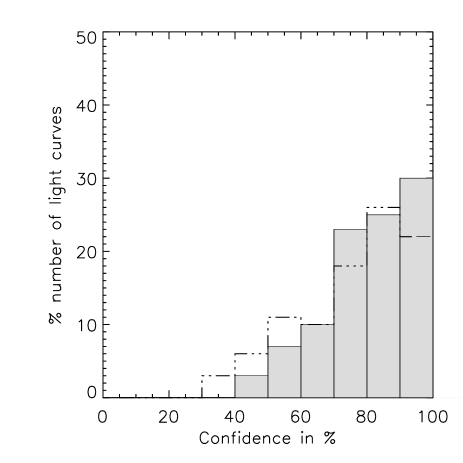
Figure 9: Distribution function for the confidence of finding the true period $T$ for a set of $100$ simulated light curves with $S/N=5$ for the range of values of transit parameters described in § 5.1). Two sets of $100$ light curves have been simulated: a set were the number of measurements per light curve is $2000$ (dotted line) and another with $4000$ measurements (solid line). Note that for the $4000$ measurements case most $T$s are recovered with confidence higher than $80$% and that for about $50$% of the simulated light curves the confidence in recovering the true period is greater than $95$%.

6 Numerical Method

The real advantage of the present method lies on the fact that for a set of light-curves most of the work can be done once in calculating the fiducial models. In this section we describe in more detail the numerical approach and we present the numerical gain over the brute force calculation using the full ${\cal X}^{2}$.

6.1 Calculations of the fiducial models

The second term of equation 13 does not depend on the actual light-curve data $\bm{x}$. Therefore, $D_{m}(\vec{q}_{f};\vec{q})$, $b_{m}^{t}(\vec{q}_{f})$ and $\beta_{m}^{t}(\vec{q}_{f})$ for each fiducial model can be pre-calculated once and stored in files. Thus for each light-curve we only need to calculate $\sum_{t}b_{m}^{t}(\vec{q}_{f})\,x^{t}$, which is independent of the search parameter $\vec{q}$. This is a major advantage of our method. Before we describe the numerical steps in more detail we need to address how we choose the fiducial models and how many fiducial models are needed.

6.2 Choice of fiducial models

There are three questions that we need to address about the choice of fiducial models.

Number of fiducial models: Since the confidence level can be calculated at each iteration step, the number of fiducial models do not need to be pre-determined. If there is only one solution at confidence larger than 70$\%$ that parameter is considered to be the correct value and the iteration is stopped. Yet, for light-curves with low S/N the actual solution may never exceed that threshold. Therefore we imposed a maximum of 100 fiducial models. Besides, for a typical survey there will be only few expected light-curves containing a transit signal, thus for most cases the iteration will be terminated at the 100 fiducial model limit.

Choice of fiducial parameters: We have found that the best performance in finding the true solution comes when we choose fiducial models from a flat distribution spanning the full range of the free parameters.

Choice of search parameters $\vec{q}$: Despite the fact that $D_{m}(\vec{q}_{f};\vec{q})$ will be calculated only once and it will not contribute to the overall computational burden of finding transits in a set of light-curves, the size of the database (files) that stores the fiducial model information heavily depends on the choice of the free parameters range and grid size. This is mostly important for future space missions where the memory available is limited.

As it can be seen from Fig. 2 (top-left panel) finding the “correct” period where there is a non linear relationship between likelihood and period is the most difficult task. This is due to the fact that a small change in the value of period $T$ produces a huge variation at the tail of the light-curve.

Theory suggests that the asymptotic standard deviation of the estimate of the period is of the order $T^{-2/3}$, so the grid should be that small too. We therefore performed the search on a uniform grid in frequency, $T^{-1}$, rather than on a uniform grid in $T$. There is also a related question of how fine the search grid should be for $\eta$ and $\tau$. Since for data folded at period $T$, the folded observation times are roughly uniform, the average spacing of subsequent folded observations is $T/N$ ($N$ is the total number of observations), $T/N$ is a natural choice for the grid size for the $\eta$ and $\tau$ searches. For a typical search the total number of searches can be as high as $10^{9}$ which translates to $1$TB of data. This is prohibiting for space missions. In what follows we examine how to further reduced the search space using physical and statistical arguments.

Transit length range: For a given period one can allow $\eta$ to take values between 0 and $T/2$. This is a naive estimate based on the fact that the planet spends half of the time in front of the star. The range of $\eta$ can be further limited using geometrical arguments and Kepler’s law. It can be shown that the transit duration is (Sackett, 1999)

$$\eta\approx\frac{T}{\pi}\sqrt{\left(\frac{R_{\star}}{a}\right)^{2}-cos^{2}(i)}$$ (23)

where $R_{\star}$ is the radius of the star, $a$ is the orbit radius of the planet and $i$ is the inclination angle. The maximum value that $\eta$ can take is when the inclination angle $i$ is zero. Using Kepler’s law the ratio of duration over period is

$$\frac{\eta}{T}=\frac{R}{\pi\,\left(\frac{T^{2}GM_{\star}}{4\pi^{2}}\right)^{1/3}}$$ (24)

For a typical main sequence star this yields a $\eta/T\approx 4\%$ for periods of 1-2 days. The fraction gets smaller as the period increases resulting a gain of factor of 50 in computational time (compared to the naive approximation $\eta/T\leq 1/2$).

Longest period: Equation 24 can be used to determine the longest period that can be recovered from the data. Namely at which period the transit duration over the period is small enough that the probability of observing more than few occultations is insignificant. It can be shown that for most inclinations the probability of observing an occultation is given by

$$p=\frac{\eta}{T}=\frac{1}{2\pi}\frac{R_{\star}}{a}\,\,.$$ (25)

This is basically the probability that the occultation time and the observation time overlap.

The probability of observing $x$ occultations during the whole lifetime of the survey is given by a binomial distribution. At the limit where the number of observations is large, the probability distribution becomes a Gaussian distribution

$$P_{t}(x)=\frac{1}{\sqrt{2\pi\,\sigma^{2}}}\exp^{-\frac{(x-\mu)^{2}}{2\,\sigma^{2}}}\,\,,$$ (26)

where $p$ is given in eq. 25. The mean value is given by

$$\mu=n_{t}\,p\,\,,$$ (27)

and the standard deviation

$$\sigma=\sqrt{n_{t}\,p\,(1-p)}\,\,.$$ (28)

where $n_{t}$ is the number of complete transits $T_{\rm range}/T$. The probability of observing at least 3 transits is therefore given by the integral

$$P(x\geq 3)=\frac{1}{\sqrt{2\pi\,\sigma^{2}}}\int_{3}^{\infty}\exp^{-\frac{(x-\mu)^{2}}{2\,\sigma^{2}}}\,dx\,\,.$$ (29)

For a typical main sequence star a planet with a period of 20 days has a probability of observing 10 occultations that is less than few percent. Using that as the upper limit to our search reduces the number of iterations by a factor 5-10.

6.3 Numerical recipe

The steps of the numerical method are described below

1. Select a set of fiducial models. The choice of the fiducial parameters span the domain of the search parameters.

2. Calculate $D_{m}(\vec{q}_{f};\vec{q})$, $b_{m}^{t}(\vec{q}_{f})$ and $\beta_{m}^{t}(\vec{q}_{f})$ for each fiducial model. The range and sampling frequency of the free parameters $\vec{q}$ are according to the physical arguments described above. Save values in a database (binary files)

3. For each light-curve calculate $\sum_{t}b_{m}^{t}(\vec{q}_{f})\,x^{t}$.

4. Search through the fiducial models for $D_{m}(\vec{q}_{f};\vec{q})$ with similar values as $\sum_{t}b_{m}^{t}(\vec{q}_{f})\,x^{t}$ from previous step. Note that since the database is sorted with respect to $D$, this is a $log(N_{q})$ operation where $N_{q}$ is the number of free parameter values.

5. Calculate $Y$ for those parameters such that $\sum_{t}b_{m}^{t}(\vec{q}_{f})\,x^{t}-D_{m}(\vec{q}_{f};\vec{q})$ is small.

6. Compute the confidence level for the selected $\vec{q}$’s using eq. 22. Note that since $D$’s, $B$’s and $\beta$’s are pre-calculated we only need to compute $\langle x\rangle$.

7. If there is only one minima with confidence level higher than 70$\%$ exit.

8. If number of fiducial models is larger than 100, exit.

9. Back to (iii).

6.4 Required number of operations

The brute force minimization for the likelihood function requires

$$N^{\rm{brute}}_{\rm{total}}\sim N_{\rm{obs}}\,N_{q}$$ (30)

The number of operations for our method after the fiducial models are computed is

$$N^{\rm MOPED+}_{\rm{total}}\sim N_{\rm{obs}}\,N_{\rm{fid}}$$ (31)

For a typical light-curve with low observing frequency like Pan-STARRS in the the four dimensional parameter space $N_{q}$ can easily be $10^{10}$. This number is large because of the non-linear dependence of the period to the likelihood, thus $N_{T}\sim 100000$ (see the arguments above). Contrary $N_{\rm{fid}}\sim 10^{2}$ which means an improvement in speed of a factor of $10^{8}$.

7 Conclusions

We have presented a new algorithm to fast and efficiently detect transits in light-curves. Our algorithm does produce a major speed up factor in light transit searches, of about eight orders of magnitude, compared to the brute force method using the full $\chi^{2}$. This translates in finding a transit on a light-curve with 10⁴ observations in well under a second on current desktop computers. We have developed a four parameter model for the transit of an object and have shown, using synthetic light-curves, that our algorithm is successful at recovering the true parameters of the transit. We have simulated a set of light-curves with the sampling rate and photometric accuracy expected in large synoptic surveys like Pan-STARRS and shown that for a large range in the values of the parameters (T, $\eta$, $\theta$, $\tau$) we recover the true values. For surveys like Pas-STARRS and LSST it should be possible to detect transits by Jovian planets and planets several times the size of earth. Since the expected detection rate of transits in this large surveys is very low, only one transit out of thousands light-curves, we believe that our method provides a fast and efficient algorithm to detect transits for future surveys.

8 ACKNOWLEDGMENTS

P. Protopapas wishes to thank Rahul Dave for valuable discussions.

References

- Aigrain & Favata (2002) Aigrain S., Favata F., 2002, A&A, 395, 625
- Alonso et al. (2004) Alonso R., et al., 2004, ApJ, 613, L153
- Charbonneau et al. (2000) Charbonneau D., Brown T. M., Latham D. W., Mayor M., 2000, ApJL, 529, L45
- Charbonneau et al. (2002) Charbonneau D., Brown T. M., Noyes R. W., Gilliland R. L., 2002, Apj, 568, 377
- Defaÿ, Deleuil, & Barge (2001) Defaÿ C., Deleuil M., Barge P., 2001, A&A, 365, 330
- Doyle et al. (2000) Doyle L. R., Deeg H. J., Kozhevnikov V. P., Oetiker B., Martín E. L., Blue J. E., Rottler L., Stone R. P. S., Ninkov Z., Jenkins J. M., Schneider J., Dunham E. W., Doyle M. F., Paleologou E., 2000, ApJ, 535, 338
- Gilliland (2000) Gilliland e. a., 2000, ApJL, 545, L47
- Heavens et al. (2000) Heavens A., Jimenez R., Lahav O., 2000, MNRAS, 317, 965
- Hoekstra et al. (2005) Hoekstra H., Wu Y., Udalski A., 2005, astro-ph/0501353
- Jenkins et al. (2002) Jenkins J. M., Caldwell D. A., Borucki W. J., 2002, ApJ, 564, 495
- Konacki et al. (2003) Konacki M., Torres G., Sasselov D. D., Jha S., 2003, ApJ, 597, 1076
- Kovács et al. (2002) Kovács G., Zucker S., Mazeh T., 2002, A&A, 391, 369
- Mallén-Ornelas et al. (2003) Mallén-Ornelas G., Seager S., Yee H. K. C., Minniti D., Gladders M. D., Mallén-Fullerton G. M., Brown T. M., 2003, ApJ, 582, 1123
- Mochejska et al. (2002) Mochejska B. J., Stanek K. Z., Sasselov D. D., Szentgyorgyi A. H., 2002, AJ, 123, 3460
- Pont et al. (2005) Pont F., et al., 2005, astro-ph/0501611
- Sackett (1999) Sackett P. D., 1999, poss.conf, 189
- Street et al. (2003) Street R. A., Horne K., Lister T. A., Penny A. J., Tsapras Y., Quirrenbach A., Safizadeh N., Mitchell D., Cooke J., Cameron A. C., 2003, MNRAS, 340, 1287
- Tingley (2003) Tingley B., 2003, A&A, 403, 329
- Torres et al. (2004) Torres G., Konacki M., Sasselov D. D., Jha S., 2004, ApJ, 614, 979
- Udalski et al. (2002) Udalski A., Paczynski B., Zebrun K., Szymaski M., Kubiak M., Soszynski I., Szewczyk O., Wyrzykowski L., Pietrzynski G., 2002, Acta Astronomica, 52, 1
- Udalski et al. (2003) Udalski A., Pietrzynski G., Szymanski M., Kubiak M., Zebrun K., Soszynski I., Szewczyk O., Wyrzykowski L., 2003, Acta Astronomica, 53, 133