Afterglow Observations Shed New Light on the Nature of X-ray Flashes

Abstract

X-ray flashes (XRFs) and X-ray rich gamma-ray bursts (XRGRBs) share many observational characteristics with long duration ($\gtrsim 2\;$s) GRBs, but the reason for which the spectral energy distribution of their prompt emission peaks at lower photon energies, $E_{p}$, is still a subject of debate. Although many different models have been invoked in order to explain the lower values of $E_{p}$, their implications for the afterglow emission were not considered in most cases, mainly because observations of XRF afterglows have become available only recently. Here we examine the predictions of the various XRF models for the afterglow emission, and test them against the observations of XRF 030723 and XRGRB 041006, the events with the best monitored afterglow light curves in their respective class. We show that most existing XRF models are hard to reconcile with the observed afterglow light curves, which are very flat at early times. Such light curves are, however, naturally produced by a roughly uniform jet with relatively sharp edges that is viewed off-axis (i.e. from outside of the jet aperture). This type of model self consistently accommodates both the observed prompt emission and the afterglow light curves of XRGRB 041006 and XRF 030723, implying viewing angles $\theta_{\rm obs}$ from the jet axis of $(\theta_{\rm obs}-\theta_{0})\sim 0.15\theta_{0}$ and $(\theta_{\rm obs}-\theta_{0})\sim\theta_{0}$, respectively, where $\theta_{0}\sim 3^{\circ}$ is the half-opening angle of the jet. This suggests that GRBs, XRGRBs and XRFs are intrinsically similar relativistic jets viewed from different angles. It is then natural to identify GRBs with $\gamma(\theta_{\rm obs}-\theta_{0})\lesssim 1$, XRGRBs with $1\lesssim\gamma(\theta_{\rm obs}-\theta_{0})\lesssim{\rm a\ few}$, and XRFs with $\gamma(\theta_{\rm obs}-\theta_{0})\gtrsim{\rm a\ few}$, where $\gamma$ is the Lorentz factor of the outflow near the edge of the jet from which most of the observed prompt emission arises. Future observations with Swift could help test this unification scheme in which GRBs, XRGRBs and XRFs share the same basic physics and differ only by their orientation relative to our line of sight.

1. Introduction

X-ray flashes (XRFs) are transient X-ray sources with durations ranging from several seconds to a few minutes and their distribution on the sky is consistent with it being isotropic (Heise et al., 2001; Kippen et al., 2003), similar to what is observed in long duration ($\gtrsim 2\;$sec) gamma-ray bursts (GRBs). XRFs are also similarly variable. They were first detected by the wide field camera (WFC) of BeppoSAX (Heise et al., 2001), and subsequently studied with HETE-II (Barraud et al., 2003; Lamb et al., 2004). In addition to XRFs, HETE-II expanded the empirical classification of variable X-ray transients to include an intermediate class of events known as X-ray rich GRBs (XRGRBs). The spectrum of XRGRBs and XRFs is similar to that of GRBs (Sakamoto et al., 2004) except for the lower values of the photon energy $E_{p}$ at which their $\nu F_{\nu}$ spectrum peaks, and the lower energy output in gamma-rays and/or X-rays, $E_{\rm\gamma,iso}$, assuming isotropic emission. In all other respects XRFs, XRGRBs and GRBs seem to form a continuum.

Many different models have been proposed for XRFs, most of which try to incorporate them in a unified scenario with GRBs. These models include high redshift GRBs (Heise et al., 2001), dirty (low $\gamma$) fireballs (Dermer, Chiang & Böttcher, 1999; Heise et al., 2001; Huang et al., 2002; Zhang, Woosley & MacFadyen, 2003; Zhang, Woosley & Heger, 2004), regular GRBs viewed off-axis (Yamazaki, Ioka & Nakamura, 2002, 2003, 2004a, 2004b; Dado, Dar, & De Rújula, 2004; Kouveliotou et al., 2004; Zhang, Woosley & Heger, 2004), photosphere dominated emission (Drenkhahn, 2002; Ramirez-Ruiz & Lloyd-Ronning, 2002; Mészáros et al., 2002), week internal shocks (low variability, $\Delta\gamma\ll\gamma$; Zhang & Mészáros, 2002a; Barraud et al., 2003; Mochkovitch et al., 2003), and large viewing angles in a structured (Lamb et al., 2005) or quasi (Zhang et al., 2004) universal jet.

Most of these models mainly aim at explaining the low values of $E_{p}$ in XRFs, and do not address their expected afterglow properties. The afterglow evolution alone can, however, serve as a powerful test for XRF models, especially after the recent discovery of several afterglows of XRFs (020427, 020903, 030723, 040701, 040825B, 040912, 040916) and XRGRB 041006. Until a few years ago, XRFs were known predominantly as bursts of X-rays, largely devoid of any observable traces at any other wavelengths. However, a striking development in the last several years through the impetus of the HETE-II satellite, has been the measurement and localization of fading X-ray and optical signals from some XRFs. These afterglow observations resulted in three redshift determinations, for XRF 020903 ($z=0.251$, Soderberg et al., 2004), XRF 040701 ($z=0.2146$, Kelson et al., 2004) and XRGRB 041006 ($z=0.716$, Fugazza et al., 2004; Price et al., 2004b). In two cases, XRF 030723 and XRGRB 041006, the afterglow light curves are reasonably well monitored from sufficiently early times so that they can be used to derive meaningful constraints on XRF models.

In this paper we critically examine the different XRF models and contrast them with the afterglow observations of XRF 030723 and XRGRB 041006, as well as other available observations such as the prompt emission characteristics and the measured distances. The paper is organized as follows. §2 describes the current empirical classification and general properties of GRB, XRGRB and XRF sources. Various XRF models are considered in §3 along with a brief discussion of the observations that support or undermine these schemes. All the models that are discussed in §3 have at least one major flaw in common: they do not naturally produce the very flat afterglow light curve seen at early times in both XRF 030723 and XRGRB 041006. In the remainder of the paper we thus concentrate only on the class of models which naturally produce such light curves. That is, a roughly uniform jet with sufficiently sharp edges viewed outside the jet core. This class of models is discussed qualitatively in §4, and more quantitatively in §5, where it is also directly compared to the prompt emission and afterglow observations of XRGRB 041006 (§5.1) and XRF 030723 (§5.2). The role of our viewing angle as an essential parameter is given particular attention. In §5.3 we briefly consider other XRFs and XRGRBs, and find that the data in these cases are too sparse and insufficient in order to derive meaningful constraints on the underlying model. Our conclusions are discussed in §6.

2. Empirical Classification of GRBs, XRGRBs & XRFs

The operational definition of an XRF by the BeppoSAX team was that of a transient source, with a duration of less than $10^{3}\;$sec, whose flux triggered the Wide Field Camera (WFC) but not the Gamma Ray Burst Monitor (GRBM). Later, with HETE-II, the definition changed slightly and was based on the ratio of the fluence in the X-ray band to that in the gamma-ray band, $f_{\rm X/\gamma}=\log_{10}[S_{\rm X}(2-30\;{\rm keV})/S_{\gamma}(30-400\;{\rm keV})]$. In addition to XRFs, an intermediate class of X-ray rich GRBs (XRGRBs) was also introduced. According to this new empirical scheme, GRBs, XRGRBs, and XRFs correspond to $f_{\rm X/\gamma}<-0.5$, $-0.5<f_{\rm X/\gamma}<0$, and $f_{\rm X/\gamma}>0$, respectively. Although the observed peak energies, $E_{p}^{\rm obs}=(1+z)^{-1}E_{p}$ (the photon energy where $\nu F_{\nu}$ peaks), are on average about a factor of $\sim 10$ less than those of the “standard” GRBs ($E_{p,{\rm XRF}}^{\rm obs}\sim 25$ keV while $E_{p,{\rm GRB}}^{\rm obs}\sim 250$ keV), the spectra of XRFs are fitted by the same Band function that is commonly used to fit GRBs (Band et al., 1993), and they seem to obey the same correlation between $E_{p}$ (that is corrected for cosmological redshift) and the isotropic energy output seen in gamma-rays (or X-rays), $E_{\rm\gamma,iso}$: $E_{p}\propto E_{\rm\gamma,iso}^{1/2}$ (Amati et al., 2002; Lloyd-Ronning & Ramirez-Ruiz, 2002; Lamb et al., 2005). While GRBs and XRFs have a different operational definition, they appear to form a continuum of events, rather than a bimodal distribution, with bursts varying uniformly from XRFs to XRGRBs to GRBs.

3. The Viability of Various XRF Models

In the next section we show that in order to reproduce the observed behavior seen in the afterglow light curves of both XRGRB 041006 and XRF 030723 a roughly uniform jet with sufficiently sharp edges viewed off-axis is required. This is a direct consequence of the very flat evolution of the afterglow light curve that is seen at early times. Such a behavior does not occur for a spherically symmetric outflow, or for a uniform jet that is viewed from within its aperture. The same also applies for a “structured” jet (Lipunov, Postnov & Prokhorov, 2001; Rossi, Lazzati & Rees, 2002; Zhang & Mészáros, 2002b) where the energy per solid angle $\epsilon$ props as the inverse square of the angle $\theta$ from the jet axis, outside of some small core angle $\theta_{c}$, $\epsilon\approx\epsilon_{0}\min[1,(\theta/\theta_{c})^{-2}]$. For most models that have been proposed in the literature to explain the phenomenology of XRFs, the afterglow light curve at early times is expected to be similar to that of a spherical flow [with $\epsilon=\epsilon(\theta_{\rm obs})$ if $\epsilon$ varies with $\theta$], and thus behave qualitatively similar to GRB afterglow light curves. Although this early afterglow behavior alone makes most XRF models inconsistent with observations, in what follows, we give additional arguments that further undermine these various schemes.

A straightforward interpretation of the low $E_{p}^{\rm obs}$ seen in both XRFs and XRGRBs is that they are in fact the high-redshift counterparts of long duration GRBs. While XRFs have on average lower energies than GRBs, their durations are comparable to those of GRBs (Heise et al., 2001), which argues against a high-redshift origin. Moreover, the recent redshift determination of XRF 020903 ($z=0.251$; Soderberg et al., 2004), XRF 040701 ($z=0.2146$, Kelson et al., 2004) and XRGRB 041006 ($z=0.716$; Fugazza et al., 2004; Price et al., 2004b) directly rules out this interpretation. Although some GRBs at very high redshifts may resemble XRFs, it is now clear that they do not represent the bulk of the population. In fact, recent estimates suggest that this high-redshift population may only constitute a small fraction of the total number of bursts, provided that the redshift distribution of GRBs accurately tracks the cosmic star formation rate of massive stars (e.g., Blain & Natarajan, 2000; Bromm & Loeb, 2002; Lloyd-Ronning, Fryer, & Ramirez-Ruiz, 2002).

Dermer, Chiang & Böttcher (1999) have pointed out that “dirty fireballs”, i.e. relativistic outflows with a larger baryonic load and hence a lower initial Lorentz factor $\Gamma_{0}$ compared to classical GRBs, would have a smaller $E_{p}$ which could be in the X-rays. When XRFs were discovered it was natural to suggest this scenario as a possible way of achieving low values for $E_{p}$ (Heise et al., 2001; Huang et al., 2002). We note here that while a lower $\Gamma_{0}$ implies a lower $E_{p}$ ($\propto\Gamma_{0}^{4}$) in the external shock model for the prompt emission, in the internal shocks model it would produce a higher $E_{p}$ ($\propto\Gamma_{0}^{-2}$). For the external shock model, the lower the observed $E_{p}=(1+z)E_{p}^{\rm obs}$ is, the lower the value of $\Gamma_{0}$ that is required to explain it. This implies that events with lower values of $E_{p}$ should have longer durations, since the deceleration time scales as $t_{\rm dec}\propto\epsilon^{1/(3-k)}\Gamma_{0}^{-2(4-k)/(3-k)}$, where $\epsilon$ is the energy per solid angle and $\rho_{\rm ext}\propto r^{-k}$. This is inconsistent with observations, as no clear trend exists between the total duration of the event and its $E_{p}$ (Sakamoto et al., 2004). What is more, as is the case in any external shock model, the afterglow should be a smooth continuation of the prompt emission as both arise from the same external shock. The observations of XRF 030723 (Fynbo et al., 2004a) offer the best evidence so far against this.

The presence of a dominant baryonic or shock pair photosphere within the standard fireball model was invoked by Ramirez-Ruiz & Lloyd-Ronning (2002) and Mészáros et al. (2002) to explain the formation of XRFs. While this is a tenable scenario for producing XRGRBs, the very low $E_{p}<5\;$keV observed for XRFs at $z\sim 0.2$ are hard to reconcile with a low-$\Gamma_{0}$, pair-dominated photospheric component (Mészáros et al., 2002).

Another way of obtaining low values of $E_{p}$ is with a roughly constant $\Gamma_{0}$ between different events, but with a small contrast in the value of $\Gamma_{0}$ between different colliding shells in the internal shocks model, $\Delta\Gamma_{0}\ll\Gamma_{0}$ (Zhang & Mészáros, 2002a; Barraud et al., 2003; Mochkovitch et al., 2003). This model, however, should produce an afterglow with an intensity that is comparable to those seen in typical GRBs. Furthermore, the isotropic equivalent kinetic energy of the afterglow shock at early times (when only the local value of $\epsilon$ along the line of sight is sampled, similar to the prompt emission) should be much larger than $E_{\rm\gamma,iso}$, because of the low radiative efficiency of the prompt emission in this scenario.

An alternative model for XRFs arises in the context of the so called universal (structured) jet models. In this class of models it is assumed that all GRB jets have the same structure, where both $\epsilon$, and $\Gamma$ depend on the angle $\theta$ with respect to the jet axis (Lipunov, Postnov & Prokhorov, 2001; Rossi, Lazzati & Rees, 2002; Zhang & Mészáros, 2002b). This model can reproduce the key features expected from the conventional on-axis uniform jet models, with the novelty being that the achromatic break time in the broadband afterglow light curves corresponds to the epoch during which the core of the jet becomes visible, rather than the edge of the jet as in the uniform jet model. For the internal shock model, which is thought to be the mechanism responsible for the prompt emission, $E_{p}\propto L_{\rm iso}^{1/2}\Gamma_{0}^{-2}$ (e.g., Ramirez-Ruiz & Lloyd-Ronning, 2002). As there is no observed correlation between the duration on an event and its $E_{p}$, this suggests that $E_{p}\propto E_{\rm\gamma,iso}^{1/2}\Gamma_{0}^{-2}$. This reproduces the observed narrow correlation $E_{p}\propto E_{\rm\gamma,iso}^{1/2}$ only if $\Gamma_{0}$ is both independent of $\theta$ and has a very small scatter between different events.

Lamb et al. (2005) have proposed a unified description of XRFs, XRGRBs and GRBs in which either (i) the half-opening angle $\theta_{0}$ of a uniform jet varies over a wide range while its energy remains constant, or (ii) our viewing angle $\theta_{\rm obs}$ with respect to a universal structured jet varies over a wide range. For convenience, we shall refer to $\theta_{0}$ and $\theta_{\rm obs}$ in these two options, , respectively, simply as $\theta_{*}$. In this picture, small values of $\theta_{*}$ correspond to GRBs, while increasingly larger values of $\theta_{*}$ correspond to XRGRBs and then to XRFs. In this scenario $E_{p}\propto\theta_{*}^{-1}$, so that the large range of observed $E_{p}$ values, ranging from $E_{p}\gtrsim 1\;$MeV for bright GRBs to $E_{p}\lesssim 5\;$keV for dim XRFs (i.e. a range of a factor of $\gtrsim 200$), directly corresponds to a similar range in $\theta_{*}$. Both the inferred values of $\theta_{*}$ from the jet break times in the afterglow light curves, and the $\log N-\log S$ distribution of BATSE GRBs (Guetta, Granot & Begelman, 2005) suggest, however, a smaller range for $\theta_{*}$, of about $\sim 10$ ($0.05\lesssim\theta_{*}\lesssim 0.5$), rather than $\gtrsim 200$.

4. Off-Axis Jet Models of GRBs & XRFs

The possibility that GRB outflows are collimated into narrow jets, where in many cases our line of sight would be outside of the jet aperture, resulting in no detectable prompt emission and an “orphan afterglows” at later times, was suggested by Rhoads (1997). This was shortly after the first detection of a GRB afterglow and before there was compelling observational evidence for jets in GRBs. As observational evidence in favor of GRB outflows being collimated into narrow jets gradually accumulated, studies of the observational signatures of off-axis GRB jets became more common (Perna & Loeb, 1998; Woods & Loeb, 1999; Moderski, Sikora & Bulik, 2000; Dalal, Griest & Pruet, 2002; Granot et al., 2002; Levinson et al., 2002; Totani & Panaitescu, 2002; Nakar, Piran & Granot, 2003; Granot & Loeb, 2003; Eichler & Levinson, 2004), again mostly devoted to orphan afterglows. The possibility that for viewing angles that are only slightly outside of the jet aperture the prompt emission might still be detectable, but would shift into the X-rays due to the reduced Doppler factor, has been pointed out by Woods & Loeb (1999). That was, however, before the discovery of XRFs. After XRFs were discovered, Yamazaki, Ioka & Nakamura (2002) suggested that GRB jets viewed slightly off-axis could naturally account for this newly discovered class of events. In later works they have significantly developed some aspects of this model (Yamazaki, Ioka & Nakamura, 2003, 2004a, 2004b), in particular those regarding the prompt emission. In this section we discuss various aspects of this model in some detail, with both the prompt and afterglow signatures being at the forefront of our attention.

4.1. The Jet Structure

The usual assumption about the jet structure is that it is perfectly uniform within some finite initial half-opening angle, $\theta_{0}$, from the jet symmetry axis, and abruptly truncates outside of $\theta_{0}$ (Woods & Loeb, 1999; Yamazaki, Ioka & Nakamura, 2002). Obviously, this is only an approximation, as physically one might expect that the jet would have a smoother outer edge, where the energy per solid angle, $\epsilon$, and the initial Lorentz factor, $\Gamma_{0}$, decrease smoothly with the angle $\theta$ from the jet symmetry axis, over some finite range in $\theta$, $\Delta\theta\gtrsim\Gamma_{0}^{-1}$. In fact, numerical simulations show that even if the jet initially has perfectly sharp edges (i.e. a ‘top hat’ jet), the interaction with the ambient medium causes its edges to become smoother with time (Granot et al., 2001). This serves as a motivation for considering a roughly uniform jet with smooth edges, as a more realistic version of the ‘top hat’ jet. The most widely used version of such a jet is one with a Gaussian angular profile for $\epsilon$ (Zhang & Mészáros, 2002b; Kumar & Granot, 2003), $\epsilon=\epsilon_{0}\exp(\theta^{2}/2\theta_{0}^{2})$. There are also other similar jet profiles, where most of the energy resides within some finite half-opening angle $\theta_{0}$, and $\epsilon$ sharply drops outside of $\theta_{0}$. Numerical simulation of a jet boring its way through a massive star progenitor in the context of the collapsar model (Zhang, Woosley & Heger, 2004) predict a roughly uniform jet core with $\theta_{0}\sim 3^{\circ}-5^{\circ}$ and wings where $\epsilon\propto\theta^{-3}$ which extend to larger angles, i.e. $\epsilon\approx\epsilon_{0}\min[1,(\theta/\theta_{0})^{-3}]$. We consider all such models to be variants of the same basic jet structure, and when viewed from outside the jet core ($\theta_{\rm obs}>\theta_{0}$) they are considered as members of the same class of XRF models. The different aforementioned variants of this jet structure are considered in §5.

4.2. The Afterglow Light Curves

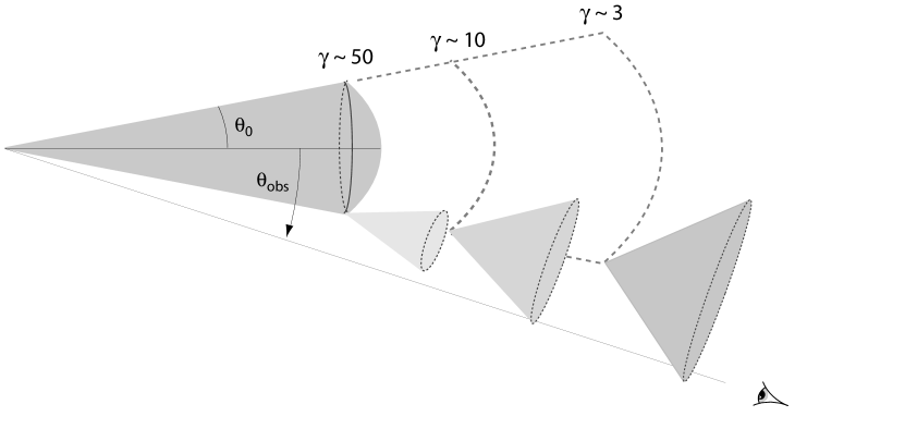
The early afterglow light curves for off-axis viewing angles ($\theta_{\rm obs}>\theta_{0}$) are generally flatter than those observed in typical on-axis ($\theta_{\rm obs}<\theta_{0}$) GRB afterglows (see Granot et al., 2002, and references therein). For a jet structure for which $\epsilon$ and $\Gamma_{0}$ drop sharply with $\theta$ at $\theta>\theta_{0}$, we expect its early light curve to rise with time. In this case, the sharper the edge of the jet, the sharper the rise in the light curve (Granot et al., 2002). For jets with sharp enough edges, the emission from the core of the jet (i.e. from $\theta<\theta_{0}$) dominates even at off-axis viewing angles ($\theta_{\rm obs}>\theta_{0}$), despite it being strongly beamed away from our line of sight (see Fig. 1). This is either because there is no emitting material along the line of sight, or even if present its emission is still weaker than that arising from the jet core. As the jet sweeps up an increasing amount of external medium, it slows down and thereafter the relativistic beaming of the emission from the jet core away from our line of sight decreases. When $\gamma$ drops to $\sim(\theta_{\rm obs}-\theta_{0})^{-1}$, our line of sight enters the beaming cone of the radiation from the jet core, causing the light curve to peak and subsequently decay, asymptotically approaching the light curve for an on-axis observer.

Figure 1.— An illustrative diagram of the emission from a uniform relativistic jet with sharp edges and half opening angle $\theta_{0}$, that is seen by an off-axis observer whose line of sight makes an angle $\theta_{\rm obs}>\theta_{0}$ with the jet axis. Because of relativistic beaming (i.e. aberration of light) the emission from each part of the jet is beamed into a narrow cone of half-opening angle $\gamma^{-1}$ around its direction of motion in the observer frame. During the prompt emission (and the very early afterglow) the Lorentz factor of the jet is large ($\gamma\gtrsim 50$) and therefore most of the radiation is strongly beamed away from the line of sight. In this case, the little radiation that is observed comes mainly from near the edge of the jet, at the point closest to the line of sight. As the jet decelerates $\gamma$ decreases with time and the beaming cone grows progressively wider, causing the radiation to be less strongly beamed, resulting in a rising light curve. The light curve peaks when $\gamma$ drops to $\sim(\theta_{\rm obs}-\theta_{0})^{-1}$ as the line of sight enters the beaming cone of the emitting material at the edge of the jet (the middle beaming cone in the figure), and subsequently decays with time, asymptotically approaching the light curve for an on-axis observer ($\theta_{\rm obs}<\theta_{0}$) at later times.

If the edge of the jet is not sufficiently sharp (i.e. if $\epsilon$ and $\Gamma_{0}$ do not drop sufficiently sharply with $\theta$ at $\theta>\theta_{0}$), then the emission from material along our line of sight may dominate over that from the core of the jet for viewing angles slightly outside the edge of the jet. In this case the light curve at early times would not rise with time, but would instead simply decay more slowly when compared to the light curve seen by on-axis observers ($\theta_{\rm obs}<\theta_{0}$). Therefore, we conclude that the jet structure, and specifically the sharpness of its edges, can be constrained by early afterglow observations. In the context of the model discussed in this section, increasingly larger viewing angles will correspond to XRGRBs and XRFs. Such a scheme is tested against observations of XRGRB 041006 and XRF 030723 in §5.

4.3. The Prompt & Reverse Shock Emission

The prompt emission for off-axis viewing angles ($\theta_{\rm obs}>\theta_{0}$) may also be dominated either by the emission from the jet core or by the emission from the material along the line of sight, depending on the viewing angle and on how sharp the edge of the jet is. If the edge of the jet is sufficiently sharp, the prompt emission is dominated by the core of the jet, and both the fluence and the peak photon energy drop sharply when compared to their on-axis values, as $[\gamma(\theta_{\rm obs}-\theta_{0})]^{-6}$ and $[\gamma(\theta_{\rm obs}-\theta_{0})]^{-2}$, respectively (Granot et al., 2002; Ramirez-Ruiz et al., 2005). The prompt emission in this case arises from the same region as for on-axis viewing angles, which in this scenario correspond to GRBs. This suggests that the same physical mechanism is responsible for the prompt emission in GRBs and in XRFs (i.e. most likely internal shocks).

If, on the other hand, the edges of the jet are not sharp enough, then the prompt emission will be dominated by material along our line of sight. As it might be hard to produce strong variability in the Lorentz factor of the outflow outside the core of the jet (Ramirez-Ruiz, Celotti & Rees, 2002; Zhang, Woosley & Heger, 2004), internal shocks may not be very efficient, and the external shock due to the interaction with the external medium might dominate the prompt emission. In that case, a smooth prompt light curve consisting of a single wide peak might be expected.

The ‘optical flash’ emission from the reverse shock is generally expected be weaker for off-axis observers (Fan, Wei & Wang, 2004). If the reverse shock is Newtonian or only mildly relativistic, then the beaming of the prompt emission (that is attributed to internal shocks within the outflow, which occur before the ejecta is decelerated by the external medium) and the reverse shock emission would not be very different. In this case the ratio of the off-axis to on-axis flux or fluence should be roughly similar for the optical flash and the prompt emission. If the reverse shock is relativistic then it would significantly decelerate the ejecta, and the emission from the reverse shock would be less strongly beamed than the prompt emission. In this case, if the emission is dominated by the jet core (i.e. for a sharp edged jet), the ‘optical flash’ emission at off-axis viewing angles could be less suppressed compared to the prompt X-ray or gamma-ray emission.

4.4. Linear Polarization

An interesting implication of the off-axis jet model for XRGRBs and XRFs is that it predicts a higher degree of linear polarization of the prompt emission, the emission from the reverse shock, and the afterglow emission, if the polarization is dominated by the jet geometry while the magnetic field is mostly tangled in the plane of the shock, as expected from the two stream instability (Medvedev & Loeb, 1999). For a shock produced magnetic field that is tangled within the shock plane, the polarization peaks at a viewing angle that satisfies $\gamma(\theta_{\rm obs}-\theta_{0})\sim 1$ (Gruzinov, 1999; Waxman, 2003; Granot, 2003; Nakar, Piran & Waxman, 2003), since at such a viewing angle most of the observed radiation is emitted roughly along the shock plane in the rest frame of the emitting plasma, due to aberration of light effects. The peak polarization can reach up to tens of percent. This is relevant to the prompt emission, and may also be relevant for the optical flash emission. The peak of the polarization which occurs at $\gamma(\theta_{\rm obs}-\theta_{0})\sim 1$ can shift to a larger viewing angle $\theta_{\rm obs}$ during the optical flash as the ejecta is decelerated by the reverse shock.

For jets with sufficiently sharp edges that are viewed off-axis, the afterglow light curve initially rises at early times, and the polarization peaks around the time of the peak in the light curve, which occurs when $\gamma(\theta_{\rm obs}-\theta_{0})$ decreases to $\sim 1$, as our line of sight enters the beaming cone of the emitting material (Granot et al., 2002). Even if there is some lateral spreading of the jet, and an initially off-axis viewing angle enters into the jet aperture as the latter grows with time, then the afterglow polarization would be relatively large, as the line of sight would still be relatively close to the edge of the jet (Sari, 1999; Ghisellini & Lazzati, 1999).

One should keep in mind, however, that ordered magnetic fields might potentially play an important role in the polarization of the prompt emission (Waxman, 2003; Granot, 2003; Nakar, Piran & Waxman, 2003; Lyutikov, Pariev & Blandford, 2003) as well as that of the reverse shock emission (the ‘optical flash’ and ’radio flare’) and the afterglow emission (Granot & Königl, 2003). If the dominant cause of polarization is an ordered magnetic field component, instead of the jet geometry together with a shock produced magnetic field, then the viewing angle would have a smaller effect on the observed linear polarization.

A recent analysis of archival ‘radio flare’ observations (Granot & Taylor, 2005) has set strong upper limits of the linear and circular polarization of this radio emission, and showed that these limits constrain the presence of an ordered magnetic field in the ejecta. The existing radio flare observations are for GRBs, which in the model considered here correspond to on-axis viewing angles ($\theta_{\rm obs}<\theta_{0}$). For a uniform jet with an ordered toroidal magnetic field, the polarization vanishes at the jet symmetry axis (i.e. for $\theta_{\rm obs}=0$) and strongly increases toward the edge of the jet. Therefore, the observed upper limits on the linear polarization translate to an upper limit on $\theta_{\rm obs}/\theta_{0}$. The best constraints so far are for GRB 991216: $P<7\%$ and $\theta_{\rm obs}/\theta_{0}\lesssim 0.4-0.55$, respectively. There are weaker constraints for GRBs 990123 and 020405. Tighter constraints on the presence of an ordered magnetic field in the ejecta are expected in the near future when a larger sample of radio flare polarization measurements becomes available. Such measurements for XRGRBs or XRFs are crucial when testing the off-axis jet model. This is because in this model one expects a viewing angle that is only slightly outside the edge of the jet and thus a large degree of polarization (tens of percent) for a purely ordered toroidal magnetic field in the ejecta.

4.5. Description of the Numerical Model

In this section we briefly describe the model that is used in §5 for describing the data. This is essentially model 1 of Granot & Kumar (2003), similar to that used by Ramirez-Ruiz et al. (2005) for modeling the lightcurve of GRB 031203. The deceleration of the flow is calculated from the mass and energy conservation equations and the energy per solid angle $\epsilon$ is taken to be independent of time. The local emissivity is calculated using the conventional assumptions of synchrotron emission from relativistic electrons that are accelerated behind the shock into a power-law distribution of energies, $N(\gamma_{e})\propto\gamma_{e}^{-p}$ for $\gamma_{e}>\gamma_{m}$, where the electrons and the magnetic field hold fractions $\epsilon_{e}$ and $\epsilon_{B}$, respectively, of the internal energy. The external density is taken to be a power law in the distance $r$ from the central source, $\rho_{\rm ext}=Ar^{-k}$, where $k=0$ corresponds to a uniform ISM while $k=2$ corresponds to a stellar wind of a massive star progenitor (assuming a constant ratio for the mass loss rate and the wind velocity). Another important physical parameter is the (true) energy of the jet, $E$, which is calculated assuming that the jet is double sided. The synchrotron spectrum is taken to be a piecewise power law (Sari, Piran & Narayan, 1998). The inverse-Compton scattering of the synchrotron photons by the same relativistic electrons, that is known as synchrotron-self Compton (SSC), is also taken into account (Panaitescu & Kumar, 2000; Sari & Esin, 2001).

The lateral spreading of the jet is neglected in this model. This approximation is consistent with results of numerical studies (Granot et al., 2001; Kumar & Granot, 2003) which show relatively little lateral expansion as long as the jet is relativistic. The light curves for observers located at different angles, $\theta_{\rm obs}$, with respect to the jet axis are calculated by applying the appropriate relativistic transformation of the radiation field from the local rest frame of the emitting fluid to the observer frame and integrating over equal photon arrival time surfaces (Granot et al., 2002; Ramirez-Ruiz & Madau, 2004).

5. Observations

The goal of this section is to quantitatively test the idea that a relativistic jet pointing slightly away from us could explain the observations of XRGRBs and XRFs. The modeling of radio, optical, and X-ray data is carried out in the framework of collimated ejecta interacting with the external medium. The model is described in §4. In this work we focus our attention on two afterglows for which radio, optical, and X-ray light curves are available: XRGRB 041006 (§5.1) and XRF 030723 (§5.2). Although, as described in §5.3, afterglow emission has also been detected for other other XRFs and XRGRBs, the data in the these cases are too sparse and insufficient in order to derive meaningful constraints on the underlying model.

5.1. X-ray Rich GRB 041006

XRGRB 041006 was detected by HETE-II (Galassi et al., 2004). It had a fluence of $5\times 10^{-6}\;{\rm erg\;cm^{-2}}$ in the $2-30\;$keV range and $7\times 10^{-6}\;{\rm erg\;cm^{-2}}$ in the $30-400\;$keV range, corresponding to $f_{X/\gamma}\approx-0.15$ which classifies it as an XRGRB. It has a redshift of $z=0.716$ (Fugazza et al., 2004; Price et al., 2004a), which for a fluence of $f\approx 1.2\times 10^{-5}\;{\rm erg\;cm^{-2}}$ in the $2-400\;$keV range gives $E_{\rm\gamma,iso}\approx 1.6\times 10^{52}\;$erg. It had an observed peak photon energy of $E_{p}^{\rm obs}=63^{+7}_{-5}\;$keV, corresponding to $E_{p}=109_{-9}^{+12}\;$keV. Figure 2 shows an off-axis model yielding an acceptable fit to the to the optical and X-ray afterglow observations of XRGRB 041006, which is also consistent with the upper limits at radio and sub-mm wavelengths (Barnard et al., 2004a, b; Soderberg & Frail, 2004). From this analysis one can conclude that a successful model for the afterglow of XRGRB 041006 is that of a collimated, misaligned jet interacting with a stellar wind external medium of mass density $\rho_{\rm ext}=Ar^{-2}$, where $r$ is the distance from the central source. The parameter values used in this fit are: $E=1.0\times 10^{51}\;$erg, $A_{*}\equiv A/(5\times 10^{11}\;{\rm gr\;cm^{-1}})=0.03$, $\theta_{0}=3^{\circ}$, $\theta_{\rm ons}=1.15\theta_{0}$, $p=2.2$, $\epsilon_{e}=0.1$, and $\epsilon_{B}=0.001$.

Figure 2.— A tentative fit to the optical R-band (shown in red; Ayani et al., 2004; Da Costa & Noel, 2004; D’Avanzo et al., 2004; Ferrero et al., 2004; Fynbo et al., 2004b; Fugazza et al., 2004; Fukushi et al., 2004; Garg et al., 2004; Greco et al., 2004; Kahharov et al., 2004; Kinoshita et al., 2004; Klotz et al., 2004; Misra & Pandey, 2004a, b; Monfardini et al., 2004; Price et al., 2004b; Yost et al., 2004) and X-ray ($0.5-6\;$keV, shown in blue; Butler et al., 2004b) light curves of XRGRB 041006. The ROTSE-IIIa points are shown with asterisk symbols since they are unfiltered, but they can still be treated as R-band observations within the measurement errors. We also added two black lines which indicate the edges of the $1\;\sigma$ confidence interval for the temporal decay index, $\alpha=1\pm 0.1$, and cover the duration of the Chandra observation. The inset shows the predicted spectral slope, $-\beta=d\log F_{\nu}/d\log\nu$, in the optical (red) and in the X-ray (blue), together with the values inferred from observations.

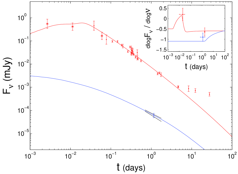
The optical light curve is very flat at early times ($\alpha\sim 0$ at $t\lesssim 1\;$hr, where $F_{\nu}\propto t^{-\alpha}\nu^{-\beta}$) and becomes steeper after a few hours ($\alpha\approx 1.2$), which is a little steeper than the decay index in the X-ray at a similar time ($\alpha\approx 1$ at $t\approx 1\;$day). Also, the ratio of the flux in the optical and X-ray at $t\approx 1\;$day implies a spectral index of $\beta\approx 0.7-0.75$ assuming a single power law between them. This suggests that the cooling break frequency $\nu_{c}$ is above the optical after $1\;$day. Since one requires very extreme parameters to get $\nu_{c}$ to the X-ray range after $1\;$day (even getting $\nu_{c}$ to be above the optical after a day requires relatively low values of $\epsilon_{B}$ and of the external density), it is most likely that $\nu_{c}$ is between the optical and X-ray at $1\;$day, which can also explain the steeper temporal decay index in the optical (by $\Delta\alpha=0.25$) for a stellar wind environment ($k=2$). This favors a wind medium over a uniform density one, since otherwise the flux in the optical will decay more slowly than in the X-ray (also by $\Delta\alpha=0.25$), which is contrary to what is observed for XRGRB 041006. At $t\gtrsim 5\;$days there is a flattening in the optical light curve, which is probably due to an underlying SN component (Garg et al., 2004). This explains why the observed flux is higher than that predicted by our narrow relativistic jet model.

The fit to the afterglow observations does not, however, uniquely determine the model parameters. Some physical parameters are nonetheless constrained better than others. The afterglow data for XRGRB 041006 requires a stellar wind environment ($k=2$) with a low density ($A_{*}\sim 0.03$) and a viewing angle that is only slightly outside the edge of the jet, $(\theta_{\rm obs}-\theta_{0})\sim 0.15\theta_{0}\sim 10^{-2}\;$rad, in order to successfully explain both the spectrum + temporal decay rates in the optical and X-ray at $\sim 1\;$day and the very flat optical light curve seen at early times.

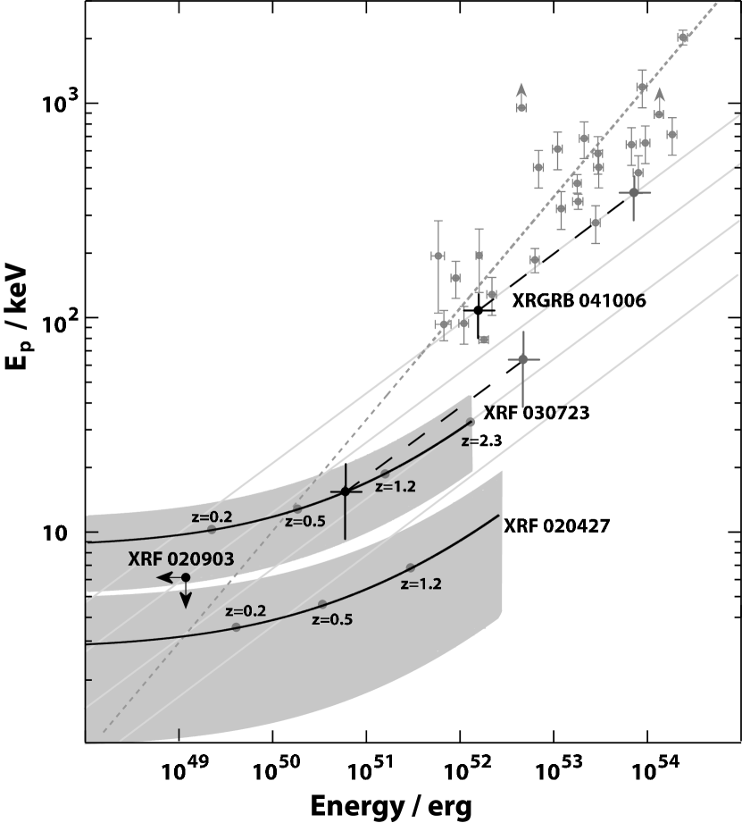
If GRB jets have well-defined edges, both the prompt gamma-ray fluence and the peak of the spectrum drop very sharply outside the opening of the jet, as $\delta^{-3}$ and $\delta^{-1}$, respectively, where $\delta\sim[\gamma(\theta_{\rm obs}-\theta_{0})]^{2}$. Therefore, the low $E_{\rm\gamma,iso}$ of XRGRB 041006 combined with $E_{\rm k,iso}=E/(1-\cos\theta_{0})\approx E(2/\theta_{0}^{2})\approx 7.3\times 10^{53}\;$erg implies $\delta\sim(E_{\rm k,iso}/E_{\rm\gamma,iso})^{1/3}\sim 3.6$ and $\gamma\sim(E_{\rm k,iso}/E_{\rm\gamma,iso})^{1/6}(\theta_{\rm obs}-\theta_{0})^{-1}\sim 240$. This implies a (cosmological) rest frame $E_{p}\sim 390\;$keV, which falls closely within the observed $E_{p}-E_{\rm\gamma,iso}$ relationship reported by Amati et al. (2002), Lloyd-Ronning & Ramirez-Ruiz (2002) and subsequently Lamb et al. (2005) using data from BeppoSAX, BATSE and HETE-II, respectively. This relationship finds that in GRBs, $E_{p}\propto E_{\rm\gamma,iso}^{1/2}$, although a significant amount of outliers may be present due to selection effects (Nakar & Piran, 2005; Band & Preece, 2005). Figure 3 shows the location of GRBs, XRFs and XRGRBs in the $E_{p}-E_{\gamma,{\rm iso}}$ plane. To date it has been difficult to extend this relationship into the XRF regime (especially at very low $E_{p}<10$ keV) since only one XRF in this spectral energy range that has a firmly established redshift (XRF 020903 at $z=0.251$; Soderberg et al., 2004). On the other hand, the existence of XRF 030723 and XRF 020427 with $E_{p}^{\rm obs}<10\;$keV is not sufficiently constraining, since their redshift is not known.

Figure 3.— XRFs in the $E_{p}-E_{{\gamma},{\rm iso}}$ plane, together with the GRBs and an X-ray rich GRBs. The compilation of observed $E_{p}$ and $E_{\gamma,{\rm iso}}$ in the source frame derived by Ghirlanda, Ghisellini & Lazzati (2004) are also illustrated. If XRGRB 041006 was viewed on-axis (at $\theta_{\rm obs}<\theta_{0}$), the peak of the spectrum and the isotropic equivalent energy would be $\sim 390\;$keV and $\sim 7.3\times 10^{53}\;$ergs, respectively (gray symbol). When viewed off-axis GRBs move in the $E_{p}-E_{{\gamma},{\rm iso}}$ plane shown in the figure along straight lines (for the log-log axis) given by $E_{p}\propto E_{{\gamma},{\rm iso}}^{1/3}$ (dashed lines).

5.2. XRF 030723

XRF 030723 was also detected by the HETE-II satellite. It had an observed peak photon energy of $E_{p}^{\rm obs}=8.4^{+3.5}_{-3.4}\;$keV and a fluence of $f\approx 5.7\times 10^{-7}\;{\rm erg\;cm^{-2}}$ in the $2-400\;$keV range (Butler et al., 2004a). No redshift determination has been made, although a firm upper limit of $z<2.3$ could be placed (Fynbo et al., 2004a). Chandra observations of the X-ray afterglow were reported by Butler et al. (2004a). In the radio band, only an upper limit of $180\;\mu$Jy was reported at $8.46\;$GHz, $3.15\;$days after the event (Soderberg, Berger & Frail, 2003).

The optical transient was discovered by Fox et al. (2003), and extensive follow up in the optical and near-infrared was reported by Fynbo et al. (2004a). The well monitored R-band light curve is initially very flat, with $\alpha\sim 0$ (where $F_{\nu}\propto t^{-\alpha}\nu^{-\beta}$). After about $1\;$day it steepens to $\alpha\approx 2$. This behavior is unusual for standard GRB light curves and allows one to constrain models of XRFs. Fynbo et al. (2004a) already noted how the early time flattening of the light curve might be an indication of an off-axis jet. Between $1-4\;$days the optical spectral slope $\beta_{\rm op}$ was in the range $\sim 1.0-1.3$, which is not unusual for GRB afterglows.

After about $\sim 10\;$days, a strong bump appeared in the optical light curve. This was assumed to be a SN component by Fynbo et al. (2004a), while Huang et al. (2004) interpreted it as an indication of a second jet, within the context of the two component jet model (see Ramirez-Ruiz, Celotti & Rees, 2002; Peng, Königl & Granot, 2005, and references therein). The bump had a sharp rise and red colors (Fynbo et al., 2004a). The sharp rise, with $\Delta t<t$, is hard to explain in both of these models, although Tominaga et al. (2004) were able to fit the sharp rise with models of SN light curves. The red colors arise naturally for a SN but are very hard to account for with a two component jet model, or for this matter also in other models for bumps in the afterglow light curve such as a density bump in the external medium, angular inhomogeneities in the jet (“patchy shell”), or a refreshed shock (Rees & Mészáros, 1998; Panaitescu et al., 1998; Ramirez-Ruiz et al., 2001b; Wang & Loeb, 2000; Ramirez-Ruiz et al., 2001a; Lazzati et al., 2002; Heyl & Perna, 2003; Nakar et al., 2003; Mészáros et al., 1998; Kumar & Piran, 2000). Therefore, the SN explanation for the bump in the optical light curve seems to be favored by the data.

Figure 4.— A tentative fit to the optical (R-band) and X-ray ($0.5-8\;$keV) light curve for XRF 030723. The first two optical points by ROTE-III are “marginal possible detections” (Smith et al., 2003), and are regarded as upper limits. We do not attempt to fit the bump in the optical at $t\gtrsim 10\;$ days, as it is attributed to a separate physical component (most likely a SN). The inset shows the spectral slope, $-\beta=d\log F_{\nu}/d\log\nu$, in the optical (blue) and in the X-ray, together with the values inferred from observations (Fynbo et al., 2004a; Butler et al., 2004a).

The X-ray light curve consists of two points, at $3.2\;$days and $13.2\;$days. A joint fit for the spectral slope at these two epoch gives $\beta_{X}=0.9^{+0.3}_{-0.2}$, while the temporal index between these two points is $\alpha_{X}=1\pm 0.1$ (Butler et al., 2004a). This is a significantly shallower decay compared to that in the optical prior to the bump ($\alpha_{\rm op}\approx 2$), and is therefore not easy to account for. Since the optical bump is most likely due to a SN component, the same physical component is not expected to contribute significantly to the X-ray flux. The shallower decay in the X-rays might be due to the contribution of synchrotron self-Compton (SSC) which can dominate the X-ray flux on time scales of days to weeks (Panaitescu & Kumar, 2000; Sari & Esin, 2001). This would generally also decrease the value of the spectral slope, $\beta_{X}$, and therefore Butler et al. (2004a) considered this option to be incompatible with the data.

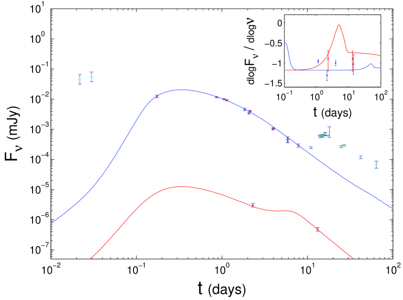
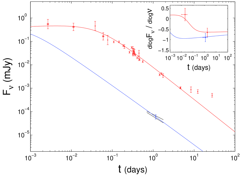
We performed a tentative fit to the data and demonstrate here that the observational constraints on the spectral slope can still be satisfied by this scenario (see Fig. 4). The physical parameters of this fit are $z=0.8$, $E=1.0\times 10^{50}\;$erg, $n=4.5\;{\rm cm^{-3}}$, $p=2.36$, $\epsilon_{B}=0.012$, $\epsilon_{e}=0.13$, $\theta_{0}=2.9^{\circ}$, $\theta_{\rm obs}=2.03\theta_{0}$. We stress that the model parameters cannot be uniquely determined from the fit to the afterglow observations, and other sets of model parameters could provide an equally good fit to the data. Some features are, however, rather robust. Most noticeable is a viewing angle of $\theta_{\rm obs}\sim 2\theta_{0}$ which is required in order to reproduce the initially very flat part of the optical light curve. A narrow jet with $\theta_{0}$ of no more than a few degrees is required in order for the jet break time $t_{j}$ to be less than about a day, which is in turn needed in order to reproduce the steep decay in the optical light curve that starts after $\sim 1\;$day.

A redshift of $z\lesssim 0.8$ is suggested by a fit of the late time bump in the optical light curve to core collapse SN light curves (Tominaga et al., 2004). This in part motivated us to choose a redshift of $z=0.8$ for the fit that we present here, but fits for other values of $z$ are also plausible. A higher $z$ would require a higher jet energy $E$, while a lower $z$ would require a smaller jet energy. For $z\approx 0.8$, $E_{\rm\gamma,iso}\approx 9.3\times 10^{50}\;$erg which together with $E_{\rm k,iso}\approx 7.8\times 10^{52}\;$erg implies $\delta\sim 4.4$ and $\gamma\sim 40$. This would in turn imply a (cosmological) rest frame $E_{p}$ of $\sim 66\;$keV if viewed on-axis, which is a factor of $\sim 3$ lower than the value required to fall exactly on the Amati relation (see Fig. 3). Given the large uncertainties associated with this relationship (Lloyd-Ronning & Ramirez-Ruiz, 2002; Nakar & Piran, 2005; Band & Preece, 2005), we consider this to be in good agreement with observations of on-axis GRBs.

It is reasonable to expect a relatively low Lorentz factor ($\gamma\sim 40$) at the edge of the jet. Assuming $\gamma$ decreases from $\gamma_{\rm int}\gtrsim 100$ in the interior of the jet to much lower values at $\Delta\theta\gtrsim 1/\gamma_{\rm int}$ centered around $\theta_{0}$, then for $\gamma\lesssim 40$ the optical depth to pair production would be large, while for larger values of $\gamma$ much fewer photons would reach and off-axis observer, so that it is reasonable that the off-axis prompt emission will be dominated by $\gamma$ for which $\tau_{\gamma\gamma}$ is just smaller than 1. A similar result was obtained in a fit to GRB 031203 (Ramirez-Ruiz et al., 2005).

Figure 5.— The R-band light curve of XRF 030723 is overlaid on top of theoretical light curves for three different jet structures, and viewing angles $\theta_{\rm obs}/\theta_{0}=0,\,0.5,\,1,\,1.5,\,2,\,2.5,\,3,\,4,\,5,\,6$. The physical parameters are the same as in Fig. 4, where the half opening angle of the uniform jet, $\theta_{0}=2.9^{\circ}$, is identified with the core angle in the two other jet structures.

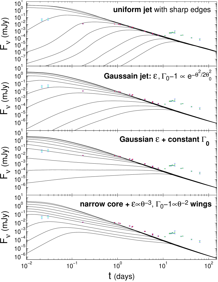
In addition to a uniform jet with sharp edges, we also consider other jet structures: (i) a narrow core with power law wings $\epsilon\approx\epsilon_{0}\min[1,(\theta/\theta_{0})^{-3}]$, $\Gamma_{0}-1\approx 299\propto\min[1,(\theta/\theta_{0})^{-2}]$, and (ii) a Gaussian jet with $\epsilon\propto\exp(-\theta^{2}/2\theta_{0}^{2})$ and either a constant $\Gamma_{0}=200$ or a Gaussian $\Gamma_{0}-1$ [i.e. $\Gamma_{0}=1+199\exp(-\theta^{2}/2\theta_{0}^{2})$]. The light curves for different viewing angles are shown in Fig. 5. For a jet with power law wings where $\epsilon\propto\theta^{-a}$ it is hard to reproduce the very flat light curve at early times that is observed in XRF 070323 (and in XRGRB 041006), even for $a\approx 3$ that is expected for the collapsar model (Zhang, Woosley & Heger, 2004), and a steeper drop in $\epsilon$ (i.e. a larger value of $a$) is required. For a Gaussian jet, the light curves have a stronger dependence on the angular profile of the initial Lorentz factor, $\Gamma_{0}(\theta)$. If it is constant, then the deceleration time at large viewing angles is still very small, and the contribution to the observed flux from material along the line of sight dominates at early times out to reasonably large viewing angle $\theta_{\rm obs}/\theta_{0}\sim{\rm a\ few}$. If, on the other hand, it has a Gaussian profile, $\Gamma_{0}-1\propto\exp(-\theta^{2}/2\theta_{0}^{2})$, then the deceleration time at large angles becomes large and the observed flux is dominated by emission from the jet core even at early times. This causes a rise in the observed flux at early times for viewing angles outside the core of the jet, similarly to a uniform jet viewed off-axis (Kumar & Granot, 2003), and in better agreement with the initially very flat light curves of XRF 070323 and XRGRB 041006. We consider a Gaussian profile for the kinetic energy per unit mass, $\Gamma_{0}-1$, to be more realistic than a constant $\Gamma_{0}$, since the latter requires a Gaussian profile for the rest mass per unit solid angle, $\mu$, that is entrained in the outflow [since $\epsilon=(\Gamma_{0}-1)\mu c^{2}$], while the former implies a constant $\mu$. If anything, one might expect $\mu$ to increase with $\theta$ rather than decrease with $\theta$ (since a larger amount of mass in the ejecta might be expected near the walls of the funnel). Thus, from the models we considered, a reasonable fit to the light curve of XRF 030723 (and XRGRB 041006) can be obtained either for a uniform jet with sharp edges viewed off-axis or for a Gaussian jet with a Gaussian profile in both $\epsilon$ and $\Gamma_{0}-1$ viewed from outside its core.

The fact that the afterglow light curve of an XRGRB requires a viewing angle that is only slightly outside the edge of the jet, while the afterglow light curve of an XRF requires a larger viewing angle ($\theta_{\rm obs}\sim 2\theta_{0}$) provides a consistent picture where a roughly uniform jet with relatively sharp edges is viewed as a GRB from within the jet aperture [i.e. $\gamma(\theta_{\rm obs}-\theta_{0})\lesssim 1$], as an XRGRB from slightly outside the edge of the jet [i.e. $1\lesssim\gamma(\theta_{\rm obs}-\theta_{0})\lesssim{\rm a\ few}$], and as an XRF from yet larger off-axis viewing angles [i.e. $\gamma(\theta_{\rm obs}-\theta_{0})\gtrsim{\rm a\ few}$].

5.3. Other events with sparse data

Besides the two events discussed above (in §5.1 and §5.2) there have been a few other XRFs with candidate afterglow detections. The data in these case are, however, too sparse to allow any meaningful constraint on theoretical models.

XRF 020903, detected by HETE-II, had an exceptionally low peak energy of $\sim 5$ KeV. Detection of the optical and radio afterglow was reported by Soderberg et al. (2004), together with the identification of the likely host galaxy at $z=0.251$. Due to the large error box, and the proximity to two other transient sources (which delayed prompt identification), the optical light curve at early times was not well sampled. The first detection is at $t=0.9\;$days after the burst, while later observations are dominated by the light from the host. In contrast to the sparse optical measurements, the radio light curve was extensively monitored with VLA over the period 25-370 days. The source, which was monitored at frequencies of 1.5, 4.9, 8.5 and $22.5\;$GHz, was found to have a temporal index $\alpha$ similar to that of “standard” GRBs (Frail et al., 2003).

XRF 020427 was detected by BeppoSAX, and no redshift measurement is available. There is a detection of X-ray emission at $t<100\;$s and a later detection at $t\sim 1\;$day. If the last of the early time detections (at $t\sim 50\;$s) is indeed marking the begin of the afterglow (as suggested by Amati et al., 2004), then the inferred steep afterglow decline would be hard to reconcile with a sharp edge seen off-axis. However, given the lack of coverage, it is not clear whether the detection at $t\sim 50\;$s is indeed part of the afterglow or, instead, still a component of the prompt emission. In the latter situation, with only one X-ray detection available, there is not much that can be said in terms of possible models.

Other cases with possible counterparts are XRF 040912, which has a candidate X-ray afterglow between $13.57\;$hr and $38.65\;$hr, and XRF 040916, which has an optical afterglow candidate but with no X-ray detection.

5.4. Supernova signatures in XRFs

The combined results on SN1998bw and SN2003dh offer the most direct evidence yet that typical, long-duration, energetic GRBs result from the deaths of massive stars (e.g., Hjorth et al., 2003; Stanek et al., 2003). The lack of hydrogen lines in both spectra is consistent with model expectations that the star lost its hydrogen envelope to become a Wolf-Rayet star before exploding. The broad lines are also suggestive of an asymmetric explosion viewed along the axis of most rapid expansion (Mazzali et al., 2001; Zhang, Woosley & Heger, 2004). Despite the rather large uncertainty on the true event rate of GRBs, a comparison with the event rate of Type Ib/c SNe suggests that only a small fraction, $f_{\rm GRB}\lesssim 10^{-3}$, of such SNe produce GRBs. The Type Ic SNe that are firmly associated with GRBs are very bright Type Ic events, with SN 1998bw being the brightest. The lack, however, of a SN in GRBs 010921 (Price et al., 2003) and 020410 (Levan et al., 2004a) to a limit of $\sim$1.5 and $\sim 2$ magnitudes fainter than SN 1998bw, respectively, suggests that we may be seeing a broader luminosity function for the Type Ic SNe that are associated with GRBs.

If the unification hypothesis discussed here is true (or in any model where GRBs and XRFs are intrinsically the same object), XRFs should be accompanied by a SN(Zhang, Woosley & Heger, 2004) brightening in their afterglow light curves, as seen in GRBs. Unfortunately, the sample of XRFs with known redshifts and optical afterglows that are sufficiently well monitored is very limited, with one possible exception – XRF 030723 which has a well sampled light curve but no measured redshift. There are, nevertheless, both upper and lower limits on the redshift of XRF 030723. A lower limit of $z\gtrsim 0.3$ has been derived from the non-detection of its host galaxy (Fynbo et al., 2004a), while an upper limit of $z<2.3$ was derived from the lack of Ly$\alpha$ absorption. Fynbo et al. (2004a) obtained optical photometry and spectroscopy of XRF 030723, and found that the optical counterpart showed a “bump” in the light curve which may be the signature of a SN component. As discussed in §5.2, the temporal and spectral energy distribution evolution are hard to reconcile with other interpretations such as a refreshed shock or a density variation in the external medium. For the redshift range $z\sim 0.3-1$, all possible SN models require a rather small mass of synthesized ⁵⁶Ni (Tominaga et al., 2004). This is because the SN brightness at this distances is $\sim 2$ magnitudes fainter than SN 1998bw. As the SN peak luminosity scales roughly linearly with its ⁵⁶Ni yield, we would expect very little ⁵⁶Ni production from a very faint SN.

The SN associated with XRF 030723 therefore appears to have properties similar to those associated with GRB 010921 and GRB 020410, i.e. it seems to lie at the low end of the hypernova luminosity function, and is perhaps even closer in its properties to a normal Type Ic SN. This might potentially be caused by our off-axis viewing angle which resulted not only in an XRF instead of a GRB, but also in a dimmer SN as opacity effects prevented us from seeing the brightest part of the SN ejecta which lies along the rotational axis. Nomoto et al. (2003) find that for the SNe that are associated with GRBs (or hypernovae), a significant decrease in luminosity may occur only for viewing angles $\theta_{\rm obs}\gtrsim 30^{\circ}$. This is a direct consequence of the anisotropic distribution of the SN ejecta. We find, however, that for XRF 030723 $\theta_{\rm obs}\sim 2\theta_{0}\sim 6^{\circ}$, which is well below $30^{\circ}$. Thus, the SN associated with XRF 030723 is probably intrinsically dimmer than SN 1998bw. Clearly, more data on the SN-GRB/XRF connection are necessary before we can understand the full extent of the relation between these phenomena.

There is already some tentative evidence that a number of XRFs (011030 and 020427), for which no optical afterglow was detected, also have no evidence for an associated SN (Levan et al., 2004b). SNe such as SN 1998bw would have been visible out to $z\sim 1.5$ in each case, while somewhat fainter SNe would have been visible to $z\sim 1$. Although it is possible that these XRFs lie at $z\gtrsim 1$, it is still puzzling given our attempt to tentatively identify GRBs, XRFs, and SNe as similar objects observed with small, medium, and large inclination, respectively.

A possibility which can explain both a relatively low redshift and the absence of a SN detection is that the afterglows were heavily dust extinguished. In the off-axis jet model, prompt and intense X-ray/UV radiation from the reverse shock may efficiently destroy and clear the dust (Waxman & Draine, 2000; Fruchter, Krolik & Rhoads, 2001; Perna & Lazzati, 2002) in the circumburst cloud within the solid angle corresponding to the initial jet aperture, i.e. at $\theta<\theta_{0}$. This implies relatively little extinction for on-axis viewing angles, $\theta_{\rm obs}<\theta_{0}$ (practically no extinction of emission from $\theta<\theta_{0}$ and a gradual increase in the extinction as $\theta$ increases above $\theta_{0}$) but a relatively large extinction for off-axis viewing angles, $\theta_{\rm obs}>\theta_{0}$, especially for emission arising from $\theta>\theta_{0}$. Interestingly enough, in this case, there could be many more obscured XRF optical afterglows, compared to GRB optical afterglows.

6. Conclusions

The existing XRF models have been examined and their predictions tested against the afterglow observations of XRF 030723 and XRGRB 041006, the events with the best monitored afterglow light curves to date within their respective class. We find that most models failed to reproduce the very flat part observed in their early afterglow light curve. This behavior is, however, naturally produced by a uniform jet viewed off-axis (i.e. from $\theta_{\rm obs}>\theta_{0}$). The edge of the jet must be sufficiently sharp, so that the emission at early times would be dominated by the core of the jet, rather than by material along the line of sight. Even for a jet with a narrow core and wings where the energy per solid angle drops as $\epsilon\propto\theta^{-3}$, as expected in the collapsar model, the afterglow light curves at early times are not quite as flat as those observed in XRF 030723 and XRGRB 041006. A Gaussian jet can produce a sufficiently flat light curve at early times as long as both $\epsilon$ and $\Gamma_{0}-1$ have a Gaussian profile (but not for a constant initial Lorentz factor $\Gamma_{0}$; see Fig. 5).

The afterglow light curve of XRGRB 041006 requires $(\theta_{\rm obs}-\theta_{0})\sim 0.15\theta_{0}\sim 0.8\times 10^{-2}\;$rad, while that of XRF 030723 requires $(\theta_{\rm obs}-\theta_{0})\sim\theta_{0}\sim 3^{\circ}\sim 0.05\;$rad. This supports a unified picture for GRBs, XRGRBs and XRFs, where they all arise from the same narrow and roughly uniform relativistic jets with reasonably sharp edges, and differ only by the viewing angle from which they are observed. Within this scheme, GRBs, XRGRBs and XRFs correspond to $\gamma(\theta_{\rm obs}-\theta_{0})\lesssim 1$, $1\lesssim\gamma(\theta_{\rm obs}-\theta_{0})\lesssim{\rm a\ few}$, and $\gamma(\theta_{\rm obs}-\theta_{0})\gtrsim{\rm a\ few}$, respectively.

The empirical classification scheme by which an event is tagged as a GRB, XRGRB or XRF (see §2) is rather arbitrary. Therefore there could be some cases where a jet that is viewed on-axis ($\theta_{\rm obs}<\theta_{0}$) will be classified as an XRGRB or XRF instead of as a GRB, or the opposite case in which a jet viewed off-axis ($\theta_{\rm obs}>\theta_{0}$) might be classified as a GRB instead of as an XRGRB or an XRF. A more physically motivated classification would be according to the ratio of the viewing angle $\theta_{\rm obs}$ and the jet half-opening angle $\theta_{0}$ [e.g., on-axis events versus off-axis events, where off-axis events could further be classified according to the value of $\gamma(\theta_{\rm obs}-\theta_{0})$], instead of relying purely on spectral characteristics as in the present empirical scheme. Such a classification would, however, be much harder to implement as it is not a trivial task to accurately determine the viewing angle.

Future observations with HETE-II and the recently launched Swift satellite, will allow us to further test this picture, and might also provide us with the necessary information to test the structure of the jet. The strongest constraints could be obtained from afterglow light curves of XRFs and XRGRBs that are well monitored from early times and at various frequencies (ranging from radio to X-rays). A useful complimentary method for constraining the jet structure is via the statistics of the observed jet break times $t_{j}$ in the afterglow light curves and the corresponding viewing angle $\theta_{\rm obs}$ in the universal structured jet model or the jet half-opening angle $\theta_{0}$ in the uniform jet model (Perna, Sari & Frail, 2003; Nakar, Granot & Guetta, 2004; Liang, Wu & Dai, 2004).

Similarly, the large statistical sample of GRBs and XRFs with redshift that will be available during the HETE-II/Swift era, will allow a reconstruction of the intrinsic luminosity function of the prompt emission. If GRBs, XRGRBs and XRFs are only a manifestation of the viewing angle for a structured, universal jet (whose wings are producing the XRFs), then no break would be expected in the luminosity function. On the other hand, if GRBs are the results of viewing angles that intersect the jet (whether structured or not), while XRFs and XRGRBs are off-axis events, then one would naturally expect a break in the luminosity function. Guetta et al. (2004) found that a luminosity function with a break is favored in order for the predicted rate of local bursts to be consistent with the observed rate. This also prevents the existence of an exceedingly large number of GRB remnants in the local Universe (Loeb & Perna, 1998; Perna, Raymond & Loeb, 2000).

The relative fraction of XRFs and XRGRBs to GRBs is also expected to be different in the various models (Lamb et al., 2005). If indeed an XRF corresponds to $\gamma(\theta_{\rm obs}-\theta_{0})\sim{\rm a\ few}$ and $(\theta_{\rm obs}-\theta_{0})\lesssim\theta_{0}$, the the solid angle from which an XRF is seen scales as $\theta_{0}/\gamma$ or as $\theta_{0}$ for a constant $\gamma$ (at a constant distance to the source), while the solid angle from which a GRB is seen scales as $\theta_{0}^{2}$. Therefore, the ratio of solid angles for GRBs and XRFs scales as $\theta_{0}$, and more GRBs compared to XRFs would be seen for larger $\theta_{0}$. As the distance to the source increases, XRFs could be detected only out to a smaller off-axis viewing angle, while most GRBs would still be bright enough to be detected out to reasonably large redshifts. Therefore, the ratio of GRBs to XRFs should increase with redshift. Finally, if the true energy $E$ in the jet is roughly constant, then the maximal redshift out to which a GRB could be detected would decrease with $\theta_{0}$ since $E_{\rm\gamma,iso}\propto\theta_{0}^{-2}$. This would increase the statistical weight of narrow jets in an observed sample, as they could be seen out to a larger volume.

We now briefly mention a few possible implication of the off-axis model for XRFs and XRGRBs. For sufficiently large viewing angles outside the edge of the jet, one might expect some decrease in the the variability of the prompt emission. This is since the width of an individual spike in the light curve scales as $\Delta t\propto\delta\sim[\gamma(\theta_{\rm obs}-\theta_{0})]^{2}$ while the peak photon energy and fluence scale as $E_{p}\propto\delta^{-1}$ and $f\propto\delta^{-3}$, respectively. Since the interval between neighboring spikes in the light curve is typically comparable to the width of an individual spike, $\Delta t$, then if $\Delta t$ increases significantly for large viewing angles this would cause at least some overlap between different pulses which would smear out some of the variability. Thus one might expect XRFs to be somewhat less variable than GRBs, at least on average, where a lower variability might be expected for lower values of $E_{p}$. This may lead to a simple physical interpretation of the observed variability-luminosity relation in the prompt gamma-ray/X-ray emission (Fenimore & Ramirez-Ruiz, 2000; Reichart et al., 2001).

Another possible signature of the off-axis model for XRFs is in the reverse shock emission. If the reverse shock is at least mildly relativistic, then the optical flash emission would be less beamed than the prompt X-ray or gamma-ray emission, due to the deceleration of the ejecta by the passage of the reverse shock. This might cause the optical flash to be suppressed by a smaller factor relative to the gamma-ray emission, compared to the corresponding on-axis fluxes. Thus XRFs or XRGRBs might still show reasonably bright optical emission from the reverse shock, which might in some cases be almost as bright as for classical GRBs. Finally, XRFs and XRGRBs might also show a larger degree of polarization compared to GRBs (see §4.4).

Figure 6.— A tentative fit to the afterglow observations of XRGRB 041006, presented in the same format as Fig. 2, but using a different theoretical model. The model used here is taken from Granot & Sari (2002), and features a spherical afterglow shock going into a stellar wind external medium ($k=2$), with $p=2.2$. It also provides an adequate description of a jet (either structured or uniform) before the jet break time (i.e. at $t<t_{j}$). The remaining four model parameters ($E_{\rm iso}$, $A_{*}$, $\epsilon_{e}$, and $\epsilon_{B}$) cannot be uniquely determined, as there are effectively only three constraints (the flux normalization and location of two break frequencies: $\nu_{m}$ and $\nu_{c}$).

An important conclusion from this study is that jet models in which $\epsilon$ and $\Gamma_{0}$ vary smoothly inside the jet, and where our lines of sight are within the jet, do not naturally reproduce the afterglow light curves of XRF 030723 and XRGRB 041006. The best example of such a model is the “universal structured jet” model (Lipunov, Postnov & Prokhorov, 2001; Rossi, Lazzati & Rees, 2002; Zhang & Mészáros, 2002b), where both $\epsilon$ and $\Gamma_{0}$ vary smoothly as a power law in $\theta$ (the usual assumption being that $\epsilon\propto\theta^{-2}$ outside of some core angle). This model fails to account for the very flat initial part of the afterglow light curves and its subsequent decay.

A possible way around this problem might be to identify the flat part of the light curve with the passage of the break frequency $\nu_{m}$ through the optical band. This should be accompanied by a change in the optical spectral slope, and should not be observed in other frequency ranges such as the radio or X-rays. For XRGRB 041006 this may actually provide a viable explanation for the data (see Fig. 6). For XRF 030723, however, a similar model fails because it does not reproduce both of the observed values of the temporal index $\alpha_{\rm op}$ (before or after the passage of $\nu_{m}$) or the observed spectral slope $\beta_{\rm op}$. One could in principle invoke both a jet break and the passage of a break frequency at roughly the same time, for a jet viewed on-axis. This would require that $\nu_{m}\sim\nu_{c}\sim\nu_{\rm op}$ at $t_{0}\sim t_{j}\sim 0.1-1\;$days, which is a large coincidence and is therefore unlikely. Even if this was the case, this assumption would be hard to reconcile with the measured optical spectral slope of $\beta_{\rm op}=0.96\pm 0.04$ at $t=1.13\;$days, as the spectral break frequencies would still be near the optical at that time, resulting in a smaller value of $\beta_{\rm op}$. The afterglow light curve of XRF 030723 therefore provides evidence against this class of models.

References

- Amati et al. (2002) Amati, L. et al. 2002, A&A, 390, 81
- Amati et al. (2004) Amati, L. et al. 2004, A&A submitted (astro-ph/0407166)
- Ayani et al. (2004) Ayani, K., et al. 2004, GCN, 2779
- Band et al. (1993) Band, D. L., et al. 1993, ApJ, 413, 281
- Band & Preece (2005) Band, D. L., & Preece R. D. 2005, submitted to ApJ (astro-ph/0501559)
- Barnard et al. (2004a) Barnard, V., et al. 2004a, GCN, 2774
- Barnard et al. (2004b) Barnard, V., et al. 2004b, GCN, 2786
- Barraud et al. (2003) Barraud, C. et al. 2003, A&A, 400, 1021
- Bikmaev et al. (2004) Bikmaev, I., et al. 2004, GCN, 2826
- Blain & Natarajan (2000) Blain, A. W., & Natarajan, P. 2000, MNRAS, 312, L35
- Bromm & Loeb (2002) Bromm, V., & Loeb, A. 2002, ApJ, 575, 111
- Butler et al. (2004a) Butler, N., Dullinghan, A., Ford, P., Ricker, G., Vanderspek, R., Hurley, K., Jernigan, J., Lamb, D., Graziani, C. 2004a, ApJ in press (astro-ph/0401020)
- Butler et al. (2004b) Butler, N., et al. 2004b, GCN, 2808
- Covino et al. (2004) Covino, S., et al. 2004, GCN, 2803
- Da Costa & Noel (2004) Da Costa, P., & Noel, N. 2004, GCN, 2789
- Dado, Dar, & De Rújula (2004) Dado, S., Dar, A. & De Rújula, A. 2004, A&A, 422, 381
- Dalal, Griest & Pruet (2002) Dalal, N., Griest, K., & Pruet, J. 2002, ApJ, 564, 209
- D’Avanzo et al. (2004) D’Avanzo, P., et al. 2004, GCN, 2788
- Dermer, Chiang & Böttcher (1999) Dermer, C. D., Chiang J., & Böttcher, M. 1999, ApJ, 513, 656
- Drenkhahn (2002) Drenkhahn, G. 2002, A&A, 387, 714
- Eichler & Levinson (2004) Eichler, D., & Levinson, A. 2004, ApJ, 614, L13
- Fan, Wei & Wang (2004) Fan, Y. Z., Wei, D. M., & Wang, C. F. 2004, MNRAS, 351, L78
- Fenimore & Ramirez-Ruiz (2000) Fenimore, E. E., & Ramirez-Ruiz, E. 2000, (astro-ph/0004176)
- Ferrero et al. (2004) Ferrero, P., et al. 2004, GCN, 2777
- Fox et al. (2003) Fox, D. B., et al. 2003, GCN, 2343
- Frail et al. (2003) Frail, D. A., Kulkarni, S. R., Berger, E. & Wieringa, M. H. 2003, AJ, 125, 2299
- Fruchter, Krolik & Rhoads (2001) Fruchter, A., Krolik, J. H., Rhoads, J. E. 2001, ApJ, 563, 597
- Fugazza et al. (2004) Fugazza, D., et al. 2004, GCN, 2782
- Fukushi et al. (2004) Fukushi, H., et al. 2004, GCN, 2767
- Fynbo et al. (2004a) Fynbo, J. P. U. et al. 2004a, preprint (astro-ph/0402240)
- Fynbo et al. (2004b) Fynbo, J. P. U. et al. 2004b, GCN, 2802
- Galassi et al. (2004) Galassi, M., et al. 2004, GCN, 2770
- Garg et al. (2004) Garg, A., et al. 2004, GCN, 2829
- Ghirlanda, Ghisellini & Lazzati (2004) Ghirlanda, G., Ghisellini, G., & Lazzati, D. 2004, ApJ in press, astro-ph/0405602
- Ghisellini & Lazzati (1999) Ghisellini, G., & Lazzati, D. 1999, MNRAS, 309, L7
- Greco et al. (2004) Greco, G., et al. 2004, GCN, 2804
- Granot (2003) Granot, J. 2003, ApJ, 596, L17
- Granot & Loeb (2003) Granot, J., & Loeb, A. 2003, ApJ, 593, L81
- Granot & Königl (2003) Granot, J., & Kónigl, A. 2003, ApJ, 594, L83
- Granot & Kumar (2003) Granot, J., Kumar, P. 2003, ApJ, 591, 1086
- Granot et al. (2001) Granot, J, Miller, M., Piran, T., Suen, W. M., & Hughes, P. A. 2001, in Gamma-Ray Bursts in the Afterglow Era, ed. E. Costa, F. Frontera, & J. Hjorth (Berlin: Springer), 312
- Granot et al. (2002) Granot, J., Panaitescu, A., Kumar, P., Woosley, S. E. 2002, ApJ, 570, L61
- Granot & Sari (2002) Granot, J., & Sari, R. 2002, ApJ, 568, 820
- Granot & Taylor (2005) Granot, J., & Taylor, G. B. 2005, ApJ in press (astro-ph/0412309)
- Granot & Ramirez-Ruiz (2004) Granot, J., & Ramirez-Ruiz, E. 2004, ApJ, 609, L9
- Gruzinov (1999) Gruzinov, A. 1999, ApJ, 525, L29
- Guetta, Granot & Begelman (2005) Guetta, D., Granot, J., & Begelman, M. C. 2005, ApJ in press (astro-ph/0407063)
- Guetta et al. (2004) Guetta, D., Perna, R., Stella, L. & Vietri, M. 2004, ApJL, 615, 73
- Heise et al. (2001) Heise, J., in’t Zand, J., Kippen, R. M., & Woods, P. M. 2001, in Proc. of the conference “Gamma-ray Bursts in the Afterglow Era”, 16
- Heyl & Perna (2003) Heyl, J. S., & Perna, R. 2003, ApJ 586, L13
- Hjorth et al. (2003) Hjorth, J., et al. 2003, Nature, 423, 847
- Huang et al. (2002) Huang, Y. F., Dai, Z. G. & Lu, T. 2002, MNRAS, 332, 735
- Huang et al. (2004) Huang, Y. F., Wu, X. F., Dai, Z. G., Ma, H. T., Lu, T. 2004, ApJ, 605, 300
- Kahharov et al. (2004) Kahharov, B., et al. 2004, GCN, 2775
- Kelson et al. (2004) Kelson, D. D., Koviak, K., Berger, E., & Fox, D. B. 2004, GCN circ. 2627
- Kinoshita et al. (2004) Kinoshita, D., et al. 2004, GCN, 2785
- Kippen et al. (2003) Kippen, R. M., et al. 2003, in Gamma-Ray Bursts ans Afterglow Astronomy, AIP Conf. Proceedings 662, ed. G. R. Ricker & R. K. Vanderspek (New York: AIP), 25
- Klotz et al. (2004) Klotz, A., et al. 2004, GCN, 2784
- Kouveliotou et al. (2004) Kouveliotou, C., et al. 2004, ApJ, 608, 872
- Kumar & Piran (2000) Kumar, P., & Piran, T. 2000, ApJ 535, 152
- Kumar & Granot (2003) Kumar, P., & Granot, J. 2003, ApJ, 591, 1075
- Lamb et al. (2004) Lamd, D. Q., et al. 2004, New Astron. Rev., 48, 423
- Lamb et al. (2005) Lamb, D., Q., Donaghy, T., Q. & Graziani, C. 2005, ApJ, 620, 355
- Lazzati et al. (2002) Lazzati, D., Rossi, E., Covino, S., Ghisellini, G., & Malesani, D. 2002, A&A 396, L5
- Levan et al. (2004a) Levan, A. et. al. 2004, ApJ in press (astro-ph/0403450)
- Levan et al. (2004b) Levan, A. et. al. 2004, ApJ in press (astro-ph/0410560)
- Levinson et al. (2002) Levinson, A., Ofek, E. O., Waxman, E., & Gal-Yam, A. 2002, ApJ, 576, 923
- Liang, Wu & Dai (2004) Liang, E. W., Wu, X. F. & Dai, Z. G. 2004, MNRAS, 354, 81
- Lipunov, Postnov & Prokhorov (2001) Lipunov, V. M., Postnov, K. A., & Prokhorov, M. E. 2001, Astron. Rep., 45, 236
- Lloyd-Ronning, Fryer, & Ramirez-Ruiz (2002) Lloyd-Ronning, N., Fryer, C., & Ramirez-Ruiz, E. 2002, ApJ, 574, 554
- Lloyd-Ronning & Ramirez-Ruiz (2002) Lloyd-Ronning, N., & Ramirez-Ruiz, E. 2002, ApJ, 576, 101
- Loeb & Perna (1998) Loeb, A. & Perna, R. 1998, ApJL, 503, 35
- Lyutikov, Pariev & Blandford (2003) Lyutikov, M., Pariev, V. I., & Blandford, R. D. 2003, ApJ, 597, 998
- Mazzali et al. (2001) Mazzali, P. A., Nomoto, K., Patat, F., & Maeda, K. 2001, ApJ, 559, 1047
- Medvedev & Loeb (1999) Medvedev, M. V., & Loeb, A. 1999, ApJ, 1999, 526, 697
- Mészáros et al. (1998) Mészáros, P., Rees, M. J., & Wijers, R. 1998, ApJ 499, 301
- Mészáros et al. (2002) Mészáros, P., Ramirez-Ruiz, E., Rees, M. J., & Zhang, B. 2002, ApJ, 578, 812
- Misra & Pandey (2004a) Misra, K., & Pandey, S. B. 2004a, GCN, 2794
- Misra & Pandey (2004b) Misra, K., & Pandey, S. B. 2004b, GCN, 2795
- Mochkovitch et al. (2003) Mochkovitch, R., Daigne, F., Barraud, C., & Atteia, J. L. 2003, ASP Conference Series (San Francisco ASP), in press (astro-phj/0303289)
- Moderski, Sikora & Bulik (2000) Moderski, R., Sikora, M., & Bulik, T. 2000, ApJ, 529, 151
- Monfardini et al. (2004) Monfardini, A., et al. 2004, GCN, 2790
- Nakar, Granot & Guetta (2004) Nakar, E., Granot J. & Guetta, D. 2004, ApJ, 606, L37
- Nakar et al. (2003) Nakar, E., Piran, T., & Granot, J. 2003, NewA 8, 495
- Nakar & Piran (2005) Nakar, E., & Piran, T. 2005, ApJ submitted (astro-ph/0412232)
- Nakar, Piran & Granot (2003) Nakar, E., Piran, T., & Granot, J. 2003, ApJ, 579, 699
- Nakar, Piran & Waxman (2003) Nakar, E., Piran, T., & Waxman, E. 2003, JCAP, 10, 5
- Nomoto et al. (2003) Nomoto, K., Maeda, K., Mazzali, P. A., Umeda, H., Deng, J. & Iwamoto, K. 2003, to appear in “Stellar Collapse” (Astrophysics and Space Science; Kluwer) ed. C. L. Fryer
- Panaitescu et al. (1998) Panaitescu, A., Mészáros, P., & Rees, M. J. 1998, ApJ 503, 314
- Panaitescu & Kumar (2000) Panaitescu, A., & Kumar, P. 2000, ApJ, 543, 66
- Peng, Königl & Granot (2005) Peng, F., Kónigl, A., & Granot, J. 2005 ,submitted to ApJ (astro-ph/0410384)
- Perna & Lazzati (2002) Perna, R. & Lazzati, D. 2002, ApJ, 580, 261
- Perna & Loeb (1998) Perna, R. & Loeb, A. 1998, 509L, 85
- Perna, Raymond & Loeb (2000) Perna, R., Raymond, J. & Loeb, A. 2000, ApJ, 533, 658
- Perna, Sari & Frail (2003) Perna, R., Sari, R. & Frail, D. 2003, ApJ, 594, 379
- Price et al. (2003) Price, P. et al. 2003, ApJ, 584, 931
- Price et al. (2004a) Price, P. A., et al. 2004a, GCN, 2771
- Price et al. (2004b) Price, P. A., et al. 2004b, GCN, 2791
- Prochasksa et al. (2004) Prochaska, J. X., et al. 2004, preprint (astro-ph/0402085)
- Ramirez-Ruiz et al. (2001a) Ramirez-Ruiz, E., Dray, L. M., Madau, P., & Tout, C. A. 2001a, MNRAS 327, 829
- Ramirez-Ruiz et al. (2001b) Ramirez-Ruiz, E., Merloni A., & Rees M. J. 2001b, MNRAS 324, 1147
- Ramirez-Ruiz, Celotti & Rees (2002) Ramirez-Ruiz, E., Celotti, A., & Rees, M. J. 2002, MNRAS, 337, 1349
- Ramirez-Ruiz & Lloyd-Ronning (2002) Ramirez-Ruiz, E., & Lloyd-Ronning, N. M. 2002, New Astron., 7, 197
- Ramirez-Ruiz & Madau (2004) Ramirez-Ruiz, E., & Madau, E. 2004, ApJ, 608, L89
- Ramirez-Ruiz et al. (2005) Ramirez-Ruiz, E., Granot, J., Kouveliotou, C., Woosley, S. E., Patel, S. K., & Mazzali, P. A. 2005, submitted to ApJL (astro-ph/0412145)
- Reichart et al. (2001) Reichart, D., Lamb, D., Fenimore, E. E., Ramirez-Ruiz, E., Cline, T., & Hurley, K. 2001, ApJ, 552, 57
- Rees & Mészáros (1998) Rees, M. J., & Mészáros, P. 1998, ApJ 496, L1
- Rhoads (1997) Rhoads, J. E. 1997, ApJ, 487, L1
- Rhoads (2003) Rhoads, J. E. 2003, ApJ, 591, 1097
- Richardson et al. (2002) Richardson, D. Branch, D., Casebeer, D., Millard, J., Thomas, R.C., Baron, E. 2002, ApJ, 123, 745
- Rossi, Lazzati & Rees (2002) Rossi, E., Lazzati, D. & Rees, M. J. 2002, MNRAS, 332, 945
- Sakamoto et al. (2004) Sakamoto, T., et al. 2004, submitted to ApJ (astro-ph/0409128)
- Sari (1999) Sari, R. 1999, ApJ, 524, L43
- Sari & Esin (2001) Sari, R., & Esin, A. A. 2001, ApJ, 548, 787
- Sari, Piran & Narayan (1998) Sari, R., Piran, T., & Narayan, R. 1998, ApJ, 497, L17
- Smith et al. (2003) Smith, D. A., Akerlof, C. W., & Quimby, R. 2003, GCN circ. 2338
- Soderberg, Berger & Frail (2003) Soderberg, A. M., Berger, E. & Frail, D. A. 2003a, GCN circ. 2330
- Soderberg et al. (2004) Soderberg, A. M., et al. 2004, ApJ, 606, 994
- Soderberg & Frail (2004) Soderberg, A. M., & Frail, D. 2004, GCN 2787
- Stanek et al. (2003) Stanek, K. Z., et al. 2003, ApJ, 591, L17
- Thomsen et al. (2004) Thomsen, B., et al. 2004, preprint (astro-ph/0403451)
- Tominaga et al. (2004) Tominaga, N., et al. 2004, ApJ, 612, L105
- Totani & Panaitescu (2002) Totani, T., & Panaitescu, A. 2002, ApJ, 576, 120
- Wang & Loeb (2000) Wang, X., & Loeb, A. 2000, ApJ 535, 788
- Waxman (2003) Waxman, E. 2003, Nature, 423, 388
- Waxman & Draine (2000) Waxman, E., & Draine, B. T. 2000 , ApJ, 537, 796
- Watson et al. (2004) Watson, D., et al. 2004, preprint (astro-ph/0401225)
- Woods & Loeb (1999) Woods, E., & Loeb, A. 1999, ApJ, 523, 187
- Yamazaki, Ioka & Nakamura (2002) Yamazaki, R., Ioka, K., & Nakamura, T. 2002, ApJ, 571, L31
- Yamazaki, Ioka & Nakamura (2003) Yamazaki, R., Ioka, K., & Nakamura, T. 2003, ApJ, 593, 941
- Yamazaki, Ioka & Nakamura (2004a) Yamazaki, R., Ioka, K., & Nakamura, T. 2004a, ApJ, 606, L33
- Yamazaki, Ioka & Nakamura (2004b) Yamazaki, R., Ioka, K., & Nakamura, T. 2004b, ApJ, 607, L103
- Yost et al. (2004) Yost, S., et al. 2004, GCN, 2776
- Zhang et al. (2004) Zhang, B., Dai, X., Lloyd-Ronning, N. M., & Mészáros, P. 2004, ApJ, 601, L119
- Zhang & Mészáros (2002a) Zhang, B. & Mészáros, P. 2002a, ApJ, 581, 1236
- Zhang & Mészáros (2002b) Zhang, B. & Mészáros, P. 2002b, ApJ, 571, 876
- Zhang, Woosley & Heger (2004) Zhang, W., Woosley, S. E., & Heger, A. 2004, ApJ, 608, 365
- Zhang, Woosley & MacFadyen (2003) Zhang, W., Woosley, S. E., & MacFadyen, A. I. 2004, ApJ, 608, 365