The Lens Galaxy In PG1115+080 is an Ellipse

Abstract

We use the structure of the Einstein ring image of the quasar host galaxy in the four-image quasar lens PG1115+080 to determine the angular structure of the gravitational potential of the lens galaxy. We find that it is well described as an ellipsoid and that the best fit non-ellipsoidal models are consistent with the ellipsoidal model. We find upper limits on the standard parameters for the deviation from an ellipse of $|a^{\rm B}_{3}/a_{0}|<0.035$ and $|a^{\rm B}_{4}/a_{0}|<0.064$. We also find that the position of the center of mass is consistent with the center of light, with an upper limit of $|\Delta\boldsymbol{x}|<0\farcs 005$ on the offset between them. Neither the ellipsoidal nor the non-ellipsoidal models can reproduce the observed image flux ratios while simultaneously maintaining a reasonable fit to the Einstein ring, so the anomalous flux ratio of the A₁ and A₂ quasar images must be due to substructure in the gravitational potential such as compact satellite galaxies or stellar microlenses rather than odd angular structure in the lens galaxy.

1. Introduction

The scenario of hierarchical structure formation dominated by cold dark matter has been extremely successful in explaining various observations of large scale structure (see, e.g., York et al. 2000; Norberg et al. 2001; Spergel et al. 2003). In this scenario, small structures form first and merge to build progressively larger structure (Rees & Ostriker, 1977; White & Rees, 1978). One prediction of these theories, both analytically and in simulations, is the existence of far more low-mass halos than are observed either in the field or as satellites of the Milky Way. Detailed studies of small satellite halos show that many survive without being tidally disrupted, albeit with some mass loss, and remain as gravitationally bound substructures in the halo of the larger galaxy (Moore et al., 1999; Klypin et al., 1999). Most estimates lead to an abundance of satellites that are inconsistent with the observed abundances, suggesting that the substructure must consist of dark satellites in which star formation was suppressed by heating and ejecting the baryons (Bullock et al., 2000). Unfortunately, dark satellite halos are difficult to detect.

Fortunately, we have one probe of halo structure that can detect substructure purely through its gravitational effects – gravitational lensing (see, e.g., Blandford & Narayan 1992; Schneider et al. 1992; Kochanek et al. 2004). Substructure in the halo of a gravitational lens galaxy, whether dark satellites or simply stars, can modify the observed fluxes of the individual images relative to those in a smooth gravitational potential. These are most striking for the systems with anomalous flux ratios between images which should have similar flux ratios given any smooth potential centered on the primary lens galaxy (e.g., Schneider & Mao 1998; Zhao & Pronk 2001; Chiba 2002; Dalal & Kochanek 2002; Metcalf & Zhao 2002). For the case of microlensing by the stars in the lens galaxy, the existence of substructure is easily verified by the temporal variations of the flux ratio such as those observed in Q2237+0305 (Woźniak et al., 2000). Tests for satellites have been focused on lensed radio sources that are too large to be affected by microlensing and little affected by the interstellar medium of the lens galaxy. Kochanek & Dalal (2004) have shown statistically at least, that the flux ratios of lenses show the characteristic pattern of demagnified saddle point images expected for low optical depths of substructure embedded in a higher optical depth of smoothly distributed dark matter (Schechter & Wambsganss, 2002; Keeton, 2003). If these anomalies are interpreted as being due to substructure, the estimated mass fraction in the substructure (Dalal & Kochanek, 2002) is consistent with theoretical expectations (Moore et al., 1999; Bullock et al., 2000). There is some debate over the contribution from small halos along the line of sight relative to those associated with the lens galaxy, with most studies favoring a dominant contribution from the lens galaxy (e.g., Metcalf 2002; Chen et al. 2003). However, from the point of view of understanding the halo mass function this is a moot point because these low mass halos are not observed as either satellites or in the field with an abundance approaching that predicted by the CDM scenario.

There have, however, been several explorations of whether the flux ratio anomalies can be explained by adding complex angular structures to the gravitational potential of the primary lens galaxy rather than by adding substructure (Evans & Witt, 2003; Kochanek & Dalal, 2004; Möller et al., 2002). In particular, Evans & Witt (2003) showed that for one particularly simple model with arbitrary angular structure the fit to the data can be reduced to a problem in linear algebra in which the lens constraints, including the flux ratios, can be modeled to arbitrary accuracy simply by including enough terms. The model parameters of this study were problematic as the quasar images needed only to be fitted to $0\farcs 05$, which is more than ten times the actual uncertainties. However, the mathematical observation that standard models fitting only the image positions fail to fit the image fluxes only because the gravitational potentials are assumed to be roughly ellipsoidal is correct. However, Kochanek & Dalal (2004) considered models with some additional angular structure and compared models constrained by either only the positions of the quasar images or the positions of the images combined with any additional constraints available for the system. In each case, the large deviations from an ellipsoidal model that could improve the modeling of the flux ratios were ruled out by the additional constraints.

In this paper we explore whether the lens galaxy in the four-image quasar lens PG1115+080 (Weymann et al., 1980; Courbin et al., 1997; Keeton & Kochanek, 1997; Impey et al., 1998; Treu & Koopmans, 2002) has significant deviations from an ellipsoidal density distribution. PG1115+080 is an interesting case because the merging A₁/A₂ images have a flux ratio of $\simeq 1.6$ rather than the ratio of $\simeq 1.0$ predicted by smooth models. We will use the same models with arbitrary angular structure considered by Evans & Witt (2003, and earlier by Witt et al. 2000; Evans & Witt 2001; Kochanek et al. 2001; Zhao & Pronk 2001) but examine the constraints imposed by the Einstein ring image of the quasar host galaxy in detail. Kochanek et al. (2001) demonstrated that the shape of the Einstein ring completely encodes the angular structure of the potential, so we can quantitatively measure the deviations of the higher order multipoles of the lens gravity from the best fit ellipsoid. In §2 we present the Hubble Space Telescope (HST) observations on which our models are based, and then briefly review our models and the fitting procedures in §3. Our main results are presented in §4, and we summarize them in §5.

Figure 1.— Einstein rings extracted from the data subsamples described in §2. Heavy solid and dotted lines represent the radius of the Einstein ring of the final combined data and its uncertainties, respectively. The four image positions are shown as filled circles.

2. HST Observations

We use the two $HST$ $H$-band (NICMOS/NIC2/F160W) images of PG1115+080. The first observation was a single-orbit (2560s) observation taken on 1997 November 17 and reported by Impey et al. (1998). The second observation was a four-orbit observation (11700s) taken on 2003 June 15. For both observations, we used four dithered sub-images per orbit to remove hot pixels and to improve the flat-fielding. The data were reduced as described in McLeod (1997) and Lehár et al. (2000). The spacecraft orientation was $69^{\circ}$ for the first observation and $-112^{\circ}$ in the second observation, so there was little change in the orientation of the quasar diffraction spikes relative to the lens.

We extracted the ring curves as described in Kochanek et al. (2001). We first fit a photometric model to the image including the four lensed quasar images, the lens galaxy and the host galaxy. This fit provides estimates of the quasar image fluxes, and these are used to subtract the lensed quasar images from the images. We then select a point close to the center of the lens, and as a function of position angle $\theta$ we find the radius $r(\theta)$ of the peak surface brightness of the Einstein ring and its uncertainties. The total number of points extracted from an Einstein ring is $N_{\rm ring}=71$. Since the ring is well-detected even in a single image, we extracted rings from several subsets of the data to explore both statistical and systematic errors in the data. We will refer to extractions from the 1997 data as obs1 and extractions from the 2003 data as obs2. For obs1 we extracted the ring using three different choices of the point about which to extract: obs1-A was centered on the lens, obs1-B was offset by $0\farcs 1$ in the $x$ direction of the image and obs1-C was offset by $0\farcs 1$ in the $y$ direction. For the obs2 data we extracted the ring for each of the four individual orbits (obs2-A, obs2-B, obs2-C and obs2-D). For our final analysis we used a ring extracted from the combined image of the four individual orbits in obs2. Figure 1 shows $r(\theta)$ for these various extractions as compared to the final combined model and its uncertainties. For the image positions and fluxes, we use the $HST$/NICMOS observations described by Impey et al. (1998).

3. Lens Model of PG1115+080

In this section, we first describe our models for the lens galaxy of PG1115+080 and the nearby galaxy group as an external perturber. Then we describe our model for the Einstein ring and our approach to fitting the data.

3.1. Lens Potential

We model the lens galaxy as a scale-free potential with arbitrary angular structure,

$$\phi(r,\theta)=rF(\theta),~{}~{}~{}~{}~{}\kappa(r,\theta)={f(\theta)\over 2r},$$ (1)

where $F(\theta)$ is an arbitrary function of angle $\theta$, and $f(\theta)=F+F^{\prime\prime}$ (Zhao & Pronk, 2001; Evans & Witt, 2001, 2003; Kochanek et al., 2001; Wucknitz, 2002). These models have a flat rotation curve, making them consistent with most estimates of the radial structure of lenses (e.g., Treu & Koopmans 2002; Rusin & Kochanek 2004). We expand the angular structure in a multipole series,

$$F(\theta)=a_{0}+\sum_{m=2}^{\infty}\left[a_{m}\cos m\theta+b_{m}\sin m\theta\right],$$ (2)

neglecting the dipole ($m=1$) terms which will be degenerate with a shift in the source position. From Poisson’s equation, the angular structure of the convergence $\kappa$ is related to that of the potential by

$$f(\theta) = a_{0}+\sum_{m=2}^{\infty}\left[a_{m}(1-m^{2})\cos m\theta+b_{m}(1-m^{2})\sin m\theta\right]$$ (3)

$$= a_{0}\left[1+\sum_{m=2}^{\infty}\left(A_{m}\cos m\theta+B_{m}\sin m\theta\right)\right],$$

where $A_{m}=(1-m^{2})a_{m}/a_{0}$ and $B_{m}=(1-m^{2})b_{m}/a_{0}$ for $m\geq 2$. We are interested in the deviations of the potential from an ellipsoidal surface mass density,

$$f(\theta)\propto\left[1-(1-q^{2})\cos^{2}\theta\right]^{-1/2}\propto 1+\sum_{m=1}^{\infty}a_{2m}^{q}\cos 2m\theta,$$ (4)

where $q$ is the axis ratio of the ellipse with coefficients $a_{2m}^{q}$ to distinguish them from the coefficients $a_{2m}$ of the general potential. We will look at deviations of the gravitational potential from an ellipsoid defined by the $a_{0}$, $a_{2}$ and $b_{2}$ coefficients. In this model, the quadrupole of the ellipsoid is defined by

$$a_{2}^{q}=-{3\over a_{0}}\left(a_{2}\cos 2\theta_{L}+b_{2}\sin 2\theta_{L}\right),$$ (5)

for axis ratio $q$ and major axis orientation $\theta_{L}=0.5\tan^{-1}(b_{2}/a_{2})$. The remainder of the coefficients $a_{2m}^{q}$ for $m\geq 2$ of the ellipsoidal model are defined by the standard multipole expansion of equation (4). We describe the rest of the model by the deviations $\Delta a_{m}$ and $\Delta b_{m}$ ($m\geq 3$) from the ellipsoid. Thus, our overall model for the primary lens is

$$F(\theta) =a_{0}+a_{2}\cos 2\theta+b_{2}\sin 2\theta$$ (6)

$$+\sum_{m=2}^{\infty}{a_{0}\over 1-4m^{2}}a_{2m}^{q}\cos 2m(\theta-\theta_{L})$$

$$+\sum_{m=3}^{\infty}\left[\Delta a_{m}\cos m\theta+\Delta b_{m}\sin m\theta\right],$$

where $a_{0}$, $a_{2}$, $b_{2}$, $\Delta a_{m}$ and $\Delta b_{m}$ are model parameters. The deviations in the mass density from the ellipsoid are $\Delta A_{m}=(1-m^{2})\Delta a_{m}/a_{0}=a^{\rm B}_{m}/a_{0}$ and $\Delta B_{m}=(1-m^{2})\Delta b_{m}/a_{0}=b^{\rm B}_{m}/a_{0}$ for $m\geq 3$ where $a^{\rm B}_{m}$ and $b^{\rm B}_{m}$ are the standard coefficients that describe the deviations of the isophotes of elliptical galaxies from ellipsoids (e.g., Bender & Möllenhoff 1987; Bender et al. 1989). Since the lens galaxy is fairly round $q_{L}\simeq 1$, we expand the ellipsoid to order $m=5$ and usually consider deviations for $m=3$ to $m=5$ beyond which the coefficients $a^{q}_{2m}$ are negligible and the perturbations are well below the noise.

3.2. The External Perturber

When modeling gravitational lens systems, it is important to include an independent external shear that can be misaligned with the light distribution (Keeton et al., 1997). In the case of PG1115+080, the dominant tidal perturbations are associated with the group to which the lens galaxy belongs (e.g., Impey et al. 1998). The group is composed of two luminous spirals and several smaller galaxies with a luminosity-weighted centroid $\sim 20\arcsec$ from the lens. Since the higher order perturbations of the group beyond an external shear are quantitatively important, we need to generalize the models of Kochanek et al. (2001) to include these higher order terms.

We model the group of galaxies as a singular isothermal sphere (SIS), $\phi_{\rm ext}=b_{g}|\boldsymbol{r}-\boldsymbol{r}_{g}|$, where $b_{g}$ is the Einstein radius of the group and $\boldsymbol{r}_{g}$ is the position vector of the group relative to the lens center. If the group is far away from the lens in the sense that $b/r_{g}\ll 1$, then we need to include only the quadratic terms in an expansion of the potential,

$$\phi_{\rm ext}(r,\theta)\simeq-{1\over 4}{b_{g}\over r_{g}}r^{2}-{1\over 4}{b_{g}\over r_{g}}r^{2}\cos 2(\theta-\theta_{g})+\mathcal{O}\left({b_{g}\over r_{g}^{2}}r^{3}\right).$$ (7)

The first term provides the mass sheet degeneracy and affects only the time delays (Falco et al., 1985; Gorenstein et al., 1988). The second term is the tidal shear, $\gamma=b_{g}/2r_{g}\simeq 0.1$ that is the dominant external perturbation (Schechter et al., 1997). However, in PG1115+080 the higher order terms are significant, so we must use a more complex model. We approximate the potential using only linear and quadratic terms in radial dependence,

$$\phi_{\rm ext}(r,\theta) \simeq r\sum_{m=1}^{\infty}a_{m}^{g}\cos m(\theta-\theta_{g})+r^{2}\sum_{m=1}^{\infty}b_{m}^{g}\cos m(\theta-\theta_{g})$$ (8)

$$\equiv rF_{\rm ext}(\theta)+r^{2}G_{\rm ext}(\theta),$$

because it has the advantage that the structure of the Einstein ring can be analytically calculated even when the potential has arbitrary angular structure. The quadratic term of the potential $G_{\rm ext}(\theta)$ is added to yield a better approximation to the radial deflections of a true SIS model. We determined the coefficients $a_{m}^{g}$ and $b_{m}^{g}$ for the external perturber by minimizing the difference in the deflection of our approximation from that of a true SIS near the Einstein ring of PG1115+080. We need to expand $\phi_{\rm ext}$ only for $m\leq 3$, and the rms deflection difference between the resulting model and a true SIS model at $r_{g}\simeq 10\arcsec$ from the lens is only $0\farcs 0005$ over a $1\arcsec$ annulus encompassing the ring. This is significantly less than our smallest astrometric errors ($0\farcs 005$).

3.3. Einstein Ring Models

We model the Einstein ring using an extension of the theory developed by Kochanek et al. (2001) for our more general potential, $\phi(r,\theta)=r\left[F(\theta)+F_{\rm ext}(\theta)\right]+r^{2}G_{\rm ext}(\theta)$. When the source is extended, the tangentially stretched images of the source form an Einstein ring. If we assume that the source has a monotonically decreasing surface brightness, the Einstein ring radius relative to the lens is simply

$$r(\theta)={\boldsymbol{h}\cdot\boldsymbol{S}\cdot\boldsymbol{t}+\boldsymbol{u}_{0}\cdot\boldsymbol{S}\cdot\boldsymbol{t}\over\boldsymbol{t}\cdot\boldsymbol{S}\cdot\boldsymbol{t}},$$ (9)

where $\boldsymbol{h}\equiv(F+F_{\rm ext})\hat{\boldsymbol{e}}_{r}+(F^{\prime}+F^{\prime}_{\rm ext})\hat{\boldsymbol{e}}_{\theta}$, the source plane tangent vector is $\boldsymbol{t}=\boldsymbol{M}^{-1}\cdot\hat{\boldsymbol{e}}_{r}=(1-2G_{\rm ext})\hat{\boldsymbol{e}}_{r}-G^{\prime}_{\rm ext}\hat{\boldsymbol{e}}_{\theta}$, $\boldsymbol{M}^{-1}$ is the inverse magnification tensor, the source center is $\boldsymbol{u}_{0}$, and $\boldsymbol{S}$ is the two-dimensional shape tensor of the source (see Kochanek et al. 2001 for the details). The only relevant parameters of the source are its axis ratio $q_{s}$ and the position angle of its major axis $\theta_{s}$.

3.4. Model Fitting

We use a simple $\chi^{2}$ statistic for the goodness of fit of a model described by parameters $\boldsymbol{p}$. The astrometric constraints consist of the observed Einstein ring radius $r(\theta_{i})$ and the four source positions $\boldsymbol{u}_{i}$. We divide the estimate into the goodness of fit to the astrometric constraints $\chi^{2}_{\rm ast}$ and the flux constraints $\chi^{2}_{\rm flux}$. The fit statistic for the astrometric constraints is

$$\chi^{2}_{\rm ast}(\boldsymbol{p})=\sum_{i}^{N_{\rm img}}{|\left[\boldsymbol{u}_{0}-\boldsymbol{u}_{i}(\boldsymbol{p})\right]M_{i}|^{2}\over\sigma_{i,{\rm img}}^{2}}+\sum_{i}^{N_{\rm ring}}{|r(\theta_{i})-r(\theta_{i};\boldsymbol{p})|^{2}\over\sigma_{i,{\rm ring}}^{2}},$$ (10)

where $M_{i}$ is the magnification of image $i$, and the $\sigma_{i}$’s are the uncertainties in either the image positions or the Einstein ring radii. The fit statistic for images is approximately correct because of the magnification weightings – the need to analyze models quickly in a large parameter space precluded using the exact image plane fit statistic. We can also constrain the model using the image fluxes, although fluxes can be contaminated by systematic errors, dust extinction, microlensing by stars, or substructure. For parity-signed fluxes $f_{i}$, we add

$$\chi^{2}_{\rm flux}(\{\boldsymbol{p},f_{s}\})=\sum_{i}^{N_{\rm img}}{|f_{i}-M_{i}(\boldsymbol{p})f_{s}|^{2}\over\sigma_{i,{\rm flux}}^{2}},$$ (11)

where the source flux $f_{s}$ is an additional free parameter of the fit.

Figure 2.— A check for systematic errors by comparing the results for the rings extracted from the data subsamples listed in the top left panel and discussed in §2. For illustration, we show the shear and PA of the group (top left), the lens galaxy position (top right), the quadrupole moment of the density distribution (lower left) and the $5\theta$ moments (lower right). The formal uncertainties in parameters are only shown for the combined data. For statistical uncertainties, the scatter in the subsamples should be twice the errorbar for the combined data.

We start by fitting the astrometric constraints with a fiducial ellipsoidal model that has 12 free parameters; the source position is $\boldsymbol{u}_{0}=(u_{x}$, $u_{y})$, the axis ratio $q_{s}$ and major-axis position angle $\theta_{s}$ of the source, the shear amplitude and the position of the external perturber $\{\gamma_{g}$, $r_{g}$, $\theta_{g}\}$, the ellipsoidal lens potential $\{a_{0}$, $a_{2}$, $b_{2}\}$, and the lens center is $(x_{L},~{}y_{L})$. Once we have estimated the goodness of fit for this model, we can add the parameters for the deviations from ellipsoidal symmetry or $\chi^{2}_{\rm flux}$, and examine the change in the goodness of fit and the parameters.

We minimize the $\chi^{2}$ of a given model and estimate the parameter uncertainties using Levenberg-Marquardt method (e.g., Press et al. 1992). We ensure that we have found a genuine $\chi^{2}$ minimum by repeating the minimization with a range of initial parameters and by checking the existence of the minimum with the downhill simplex method. We tested the code on a range of synthetic lenses with Einstein rings including both ellipsoidal and non-ellipsoidal models.

As a last step before presenting our results, we fit rings extracted from subsamples of the data as a check for systematic errors, and the level of our random errors. We consider the standard ring from obs1 extracted in three different positions relative to the lens galaxy (obs1-ABC) and the rings extracted from the four individual orbits of obs2 (obs2-ABCD). In each case the lens was re-modeled as part of the extraction procedure. Unfortunately, the rotation of the PSF between the two observations is negligible (see §2), so comparisons of the data sets provide little constraint on systematic errors arising from the PSF. Figure 2 compares the results for these seven data sets for a range of variables using the full non-ellipsoidal models. The main point to note is that the parameter estimates are mutually consistent. Also note that the distributions of the parameter estimates are consistent with the formal statistical uncertainties, except for the 5th order deviations where they are smaller. For the remainder of the paper we consider only the combined data.

Table 1Best-Fit Models

	Ellipsoidal Model			Non-Ellipsoidal Model
Parameter	Astrometry Only	Astrometry+Flux		Astrometry Only	Astrometry+Flux
$q_{s}$	0.69(02)	0.69(02)		0.70(02)	0.68(03)
$\theta_{s}$(degrees)	$-$32.0(2.7)	$-$30.9(2.6)		$-$33.4(4.6)	$-$30.9(3.6)
$\gamma_{g}$	0.116(01)	0.112(01)		0.112(03)	0.112(02)
$r_{g}$(arcsec)	10.8(1.4)	12.4(1.8)		16.9(12.5)	12.5(7.1)
$\theta_{g}$(degrees)	$-$113(00)	$-$116(00)		$-$113(01)	$-$116(01)
$x_{L}$(arcsec)	0.001(02)	0.005(02)		$-$0.003(03)	0.008(03)
$y_{L}$(arcsec)	0.001(01)	0.001(01)		$-$0.002(03)	0.004(03)
$q_{L}$	0.97(02)	0.98(01)		0.96(03)	0.99(02)
A1/A2	0.97(03)	0.94(02)		1.00(13)	0.93(06)
$\theta_{L}$(degrees)	$-66.1$(7.8)	68.4(4.9)		$-$52.4(9.2)	61.8(26.1)
$a_{0}$	1.15(00)	1.15(00)		1.15(01)	1.15(00)
$10^{3}a_{2}$	$4.1(2.0)$	$-3.2(0.9)$		$2.2(2.7)$	$-1.0(1.7)$
$10^{3}b_{2}$	$4.5(1.1)$	$3.0(0.6)$		$8.3(3.4)$	$1.5(1.5)$
$10^{3}\Delta a_{3}$	$\equiv 0$	$\equiv 0$		$-1.4(4.6)$	$0.4(1.7)$
$10^{3}\Delta b_{3}$	$\equiv 0$	$\equiv 0$		$0.8(7.2)$	$0.5(2.7)$
$10^{3}\Delta a_{4}$	$\equiv 0$	$\equiv 0$		$-0.1(4.6)$	$-0.7(1.3)$
$10^{3}\Delta b_{4}$	$\equiv 0$	$\equiv 0$		$0.3(5.7)$	$-0.3(1.2)$
$10^{3}\Delta a_{5}$	$\equiv 0$	$\equiv 0$		$-0.2(1.9)$	$0.4(1.6)$
$10^{3}\Delta b_{5}$	$\equiv 0$	$\equiv 0$		$0.3(1.1)$	$0.1(0.7)$
$\chi^{2}_{\rm ring}$	35.6	38.1		29.3	41.6
$\chi^{2}_{\rm image}$	0.2	5.4		0.1	5.4
$\chi^{2}_{\rm lens}$	0.1	2.8		1.6	9.2
$\chi^{2}_{\rm flux}$	$-$	45.4		$-$	28.7
$\chi^{2}_{\rm tot}$	36.0	91.7		31.1	84.8

Note. — The best fit ellipsoidal and non-ellipsoidal ($m=5$) models of PG1115+080, fitting either only the astrometric constraints or the astrometric constraints and the observed flux ratios. All the angles are standard position angles while the lens position and the coefficients of the lens potential are calculated in Cartesian coordinates in which $x$-direction is toward west. The errors are shown in parentheses.

Figure 3.— The best fit ellipsoidal (heavy lines) and $m=5$ non-ellipsoidal (light lines) models for the ring based on the astrometric constraints. The observed positions of the Einstein ring and the lensed images are represented as open circles and triangles, respectively. The line sizes of the open circles are the positional uncertainties of the Einstein ring radius while the uncertainties in the image positions ($0\farcs 003$) are omitted. The filled circles represent the Einstein ring positions of the best fit ellipsoidal model, while the filled ellipse at the center shows the predicted position, ellipticity and position angle of the source. The heavy solid and dashed lines show the critical line (solid) and the isodensity curve (dashed) of the ellipsoidal model, while the corresponding curves of the best-fit non-ellipsoidal model are shown with the light lines.

4. Results

In this section we address three issues. First, is the lens consistent with an ellipsoid when we fit only the astrometric constraints? Second, is the center of mass consistent with the center of light? Third, are any of these conclusions changed if we try to fit the flux ratios as well?

4.1. Is the Lens an Ellipsoid?

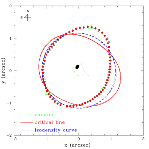
We start by fitting only the astrometric constraints, first with a purely ellipsoidal model, and then adding deviations. The results are presented in Table 1. An ellipsoidal model with a very round lens ($q_{L}\simeq 1$), a group located at a position angle of $\theta_{g}\simeq-113^{\circ}$ and at a distance of $r_{g}\simeq 11\arcsec$ provides a reasonable fit to our data and is consistent with the earlier models using a singular isothermal ellipsoid for the lens (Schechter et al., 1997; Keeton & Kochanek, 1997; Courbin et al., 1997; Impey et al., 1998; Zhao & Pronk, 2001; Kochanek & Dalal, 2004). The total $\chi^{2}_{\rm tot}\simeq 36$ for 69 degrees of freedom means that we have somewhat overfit the data and/or overestimated the uncertainties by 38%. Figure 3 shows the best fit ellipsoidal model using only the astrometric constraints.

Next, we fit the data using a sequence of non-ellipsoidal models to investigate how much the lens can deviate from ellipsoidal. We did this by sequentially including higher order poles starting with $m=3$ ($\Delta a_{3}$, $\Delta b_{3}$), then $m=4$ and finally $m=5$. For comparison with the ellipsoidal model, we show the critical line and the isodensity curve of the best fit $m=5$ non-ellipsoidal model in Figure 3, and we present their final parameters in Table 1. It is particularly interesting to note that all the higher order deviations are consistent with zero.

We summarize the resulting $\chi^{2}$ of each model in Table 2. We use the F-test to estimate whether the new parameters significantly improve the fit, and we find that none of the new variables significantly improves the models. In many cases, adding the new variables even raises the $\chi^{2}$ per degree of freedom. All the best fit non-ellipsoidal models are consistent with the best fit ellipsoidal model. In short, the constraints on the angular structure from the Einstein ring force the lens of PG1115+080 to be consistent with an ellipsoidal density. The isophotal deviations of the best fit non-ellipsoidal models are $\sim 10^{-3}$ for both $a^{\rm B}_{m}$ and $b^{\rm B}_{m}$ ($m\leq 5$) somewhat smaller than the values of $a^{\rm B}_{3}/a_{0}=0.009$, $a^{\rm B}_{4}/a_{0}=-0.004$ for $H$-band, and $a^{\rm B}_{3}/a_{0}=-0.015$, $a^{\rm B}_{4}/a_{0}=-0.004$ for $I$-band found by Evans & Witt (2003).

In our first models, we constrained the center of mass to agree with the observed lens position and its formal uncertainties of $0\farcs 003$. Evans & Witt (2003) were concerned that the center of light and mass may differ, and allowed the lens center enormous freedom to move relative to the observed position (0$\farcs$05). For our next experiment, we drop the constraint on the lens position and re-optimize the models. We find a lens position of ($-0\farcs 001\pm 0\farcs 002$, $-0\farcs 001\pm 0\farcs 002$) compared to the measured position of ($0\farcs 000\pm 0\farcs 003$, $0\farcs 000\pm 0\farcs 003$) or a net difference of $0.3\sigma$ for the RA and $0.4\sigma$ for the Dec. The center of mass of the lens is essentially identical to the center of light. The observed lens galaxy of PG1115+080 has an axis ratio $q\simeq 0.9$ and a position angle $\theta\simeq-70^{\circ}$ (Impey et al., 1998; Falco et al., 2000). The best-fit axis ratio $q_{L}$ of the mass is rounder than the light while the position angle $\theta_{L}$ is aligned with the light for both the elliptical and non-elliptical models.

Table 2F-Tests of The Additional Degrees of Freedom

	Astrometry only (A)					Astrometry+Flux (F)
Model ($m$)	$N_{par}$	dof	$\chi^{2}_{dof}$	P(%)		$N_{par}$	dof	$\chi^{2}_{dof}$	P(%)
0	12	69	0.522	100		13	72	1.273	100
3	14	67	0.474	69.1		15	70	1.310	90.5
4	16	65	0.488	78.7		17	68	1.301	92.7
5	18	63	0.493	82.0		19	66	1.285	96.6

Note. — Using astrometric constraints only, models with higher order deviations (A$m$) for order $\cos m\theta$ are compared to the fiducial ellipsoidal model (A0). When flux constraints are added, models (F$m$) for order $\cos m\theta$ are compared to F0. The dof column gives the number of degrees of freedom and the $\chi^{2}_{dof}$ column gives the $\chi^{2}$ per degree of freedom. The probability P gives the F-test probability that a given non-ellipsoidal model is consistent with ellipsoidal model. A non-ellipsoidal model with lower P implies a more significant improvement relative to the ellipsoidal model – none of the improvements is significant.

4.2. The Flux Ratio Anomalies

Because we believe the anomalous flux ratios are due to substructure (satellites or stars) rather than a problem in the lens model, we have so far neglected the flux ratios as a model constraint. We now investigate the changes in the lens potential when the flux constraints are added. The best fit parameters of an ellipsoidal model with flux constraints are also shown in Table 1. There is little change from the parameters of the ellipsoidal model based only on the astrometric constraints. As expected, most of the contribution to the fit statistic $\chi^{2}_{\rm flux}$ comes from the merging A₁/A₂ image pair showing the well-known flux anomaly. To reproduce the observed flux ratios, the critical line should be either distorted or moved closer to the brightest image so that the flux ratio becomes higher than predicted by ellipsoidal models. In the Evans & Witt (2003) models, this was possible because the quasar and lens positions could be shifted by far more than their actual uncertainties. However, with the correct QSO uncertainties and the Einstein ring constraints, especially on the angular structure of the lens potential, the best fit model with the flux constraints largely coincides with that using the astrometric constraints only.

We then added the higher order deviations from an ellipsoid and fit the data with non-ellipsoidal models. Since the magnification, $M\propto F^{\prime\prime}\propto m^{2}a_{m}$, is more sensitive to the higher order multipoles, the best-fit non-ellipsoidal models produce a better fit to the flux ratios, but it is still impossible to significantly improve flux ratios while simultaneously maintaining a good fit to the Einstein ring. The best fit model with flux constraints is still consistent with the ellipsoidal model. The fit statistics and the F-test results are shown again in Table 2. Note that the major axis of the mass is misaligned with the light when we use the flux ratios as a model constraint.

5. Summary

We modeled the lensed quasar images and the Einstein ring formed from its host galaxy in the lens PG1115+080 using a scale-free potential with arbitrary angular structure. The best fit ellipsoidal model is consistent with previous results, and provides a reasonable fit to the astrometric constraints of both the Einstein ring and the images. Non-ellipsoidal models are constructed by adding higher-order deviations from the ellipsoidal model, but none of the additional degrees of freedom improves the models. The best-fit non-ellipsoidal models are still consistent with the best fit ellipsoidal model. We also find that the center of mass of the lens is consistent with the measured center of light even when this is not imposed as a constraint.

When we try to fit the fluxes as well, including the anomalous A₁/A₂ flux ratio, the best-fit non-ellipsoidal models still fail to match the observed flux ratios and are still consistent with the ellipsoidal model. We conclude that the suggestions that complex angular structure in the lens galaxy can explain the anomalous flux ratio in PG1115+080 are incorrect – the galaxy is indistinguishable from an ellipsoid. This result does not address the problem of whether the anomaly is due to microlensing or satellites and whether the source of substructure is in the lens or along the line of sight. The predicted A₁/A₂ flux ratio for the astrometry only models is $0.97\pm 0.03$ (see Tab.1). There is some evidence that the emission line flux ratios are closer to this value (Popović & Chartas, 2005), suggesting that the anomaly is due to microlensing rather than satellite despite the lack of time variations in the ratio. Since Einstein rings are relatively common in $H$-band $HST$ observations of lenses, we should be able to test the ellipsoidal hypothesis in many additional systems.

References

- Bender & Möllenhoff (1987) Bender, R., & Möllenhoff, C. 1987, A&A, 177, 71
- Bender et al. (1989) Bender, R., Surma, P., Döbereiner, S., Möllenhoff, C., & Madejsky, R. 1989, A&A, 217, 35
- Blandford & Narayan (1992) Blandford, R., & Narayan, R. 1992, ARAA, 30, 311
- Bullock et al. (2000) Bullock, J. S., Kravtsov, A. V., & Weinberg, D. H. 2000, ApJ, 539, 517
- Chen et al. (2003) Chen, J., Kravtsov, A. V., & Keeton, C. R. 2003, ApJ, 592, 24
- Chiba (2002) Chiba, M. 2002, ApJ, 565, 17
- Courbin et al. (1997) Courbin, F., Magain, P., Keeton, C. S., Kochanek, C. S., Vanderriest, C., Jaunsen, A. O., & Hjorth, J. 1997, A&A, 324, 1
- Dalal & Kochanek (2002) Dalal, N., & Kochanek, C. S. 2002, ApJ, 572, 25
- Evans & Witt (2001) Evans, N. W., & Witt, H. J. 2001, MNRAS, 327, 1260
- Evans & Witt (2003) Evans, N. W., & Witt, H. J. 2003, MNRAS, 345, 1351
- Falco et al. (1985) Falco, E. E., Gorenstein, M. V., & Shapiro, I. I. 1985, ApJ, 289, L1
- Falco et al. (2000) Falco, E. E., et al. 2000, in Gravitational Lensing: Recent Progress and Future Goals, ed. T. G. Brainerd & C. S. Kochanek (San Francisco: ASP)
- Gorenstein et al. (1988) Gorenstein, M. V., Falco, E. E., & Shapiro, I. I. 1988, ApJ, 327, 693
- Impey et al. (1998) Impey, C. D., Falco, E. E., Kochanek, C. S., Lehár, J., McLeod, B. A., Rix, H.-W., Peng, C. Y.,& Keeton, C. R. 1998, ApJ, 509, 551
- Keeton (2003) Keeton, C. R. 2003, ApJ, 584, 664
- Keeton & Kochanek (1997) Keeton, C. S., & Kochanek, C. S. 1997, ApJ, 487, 42
- Keeton et al. (1997) Keeton, C. S., Kochanek, C. S., & Seljak, U. 1997, ApJ, 482, 604
- Klypin et al. (1999) Klypin, A., Kravtsov, A. V., Valenzuela, O., & Prada, F. 1999, ApJ, 522, 82
- Kochanek & Dalal (2004) Kochanek, C. S., & Dalal, N. 2004, ApJ, 610, 69
- Kochanek et al. (2001) Kochanek, C. S., Keeton, C. R., & McLeod, B. A. 2001, ApJ, 547, 50
- Kochanek et al. (2004) Kochanek, C. S., Schneider, P., & Wambsganss, J. 2004, Gravitational Lensing: Strong, Weak & Micro, Proceedings of the 33rd Saas-Fee Advanced Cource, G. Meylan, P. Jetzer & P. North, eds. (Springer-Verlag: Berlin, astro-ph/0407232)
- Lehár et al. (2000) Lehár, J., et al. 2000, ApJ, 536, 584
- McLeod (1997) McLeod, B. A. 1997, in 1997 HST Calibration Workshop, ed. S. Casertano et al., Space Telescope Institute, 281
- Metcalf (2002) Metcalf, R. B. 2002, ApJ, 580, 696
- Metcalf & Zhao (2002) Metcalf, R. B., & Zhao, H.-S. 2002, ApJ, 567, L5
- Möller et al. (2002) Möller, O., Natarajan, P., Kneib, J.-P., & Blain, A. W. 2002, ApJ, 573, 562
- Moore et al. (1999) Moore, B., Ghigna, S. Governato, F., Lake, G., Quinn, T., Stadel, J., & Tozzi, P. 1999, ApJ, 524, L19
- Norberg et al. (2001) Norberg, P., et al. 2001, MNRAS, 328, 64
- Popović & Chartas (2005) Popović, L. Č., & Chartas, G. 2005, MNRAS, 357, 135
- Press et al. (1992) Press, W. H., Flannery, B. P., Teukolsky, S. A., & Vetterling, W. T. 1992, Numerical Recipes (Cambridge: Cambridge Univ. Press)
- Rees & Ostriker (1977) Rees, M. J., & Ostriker, J. P. 1977, MNRAS, 179, 541
- Rusin & Kochanek (2004) Rusin, D., & Kochanek, C. S. 2004, ApJ, submitted (astro-ph/0412001)
- Schechter et al. (1997) Schechter, P. L., et al. 1997, ApJ, 475, L85
- Schechter & Wambsganss (2002) Schechter, P. L., & Wambsganss, J. 2002, ApJ, 580, 685
- Schneider et al. (1992) Schneider, P., Ehlers, J., & Falco, E. E. 1992, Gravitational Lenses, (Berlin: Speringer-Verlag)
- Schneider & Mao (1998) Schneider, P., & Mao, S. 1998, MNRAS, 295, 587
- Spergel et al. (2003) Spergel, D. N., et al. 2003, ApJS, 148, 175
- Treu & Koopmans (2002) Treu, T., & Koopmans, L. V. E. 2002, ApJ, 575, 87
- Weymann et al. (1980) Weymann, R. J., et al. 1980, Nature, 285, 641
- White & Rees (1978) White, S. D. M., & Rees, M. J. 1978, MNRAS, 183, 341
- Witt et al. (2000) Witt, H. J., Mao, S., & Keeton, C. R. 2000, ApJ, 544, 98
- Woźniak et al. (2000) Woźniak, P. R, Alard, C., Udalski, A., Szymański, M., Kubiak, M., Pietrzyński, G., & Żebruń, K. 2000, ApJ, 529, 88
- Wucknitz (2002) Wucknitz, O. 2002, MNRAS, 332, 951
- York et al. (2000) York, D., et al. 2000, AJ, 120, 1579
- Zhao & Pronk (2001) Zhao, H. S., & Pronk, D. 2001, MNRAS, 320, 401